Thermal Treatment of the Minority Game

Abstract

We study a cost function for the aggregate behavior of all the agents involved in the Minority Game (MG) or the Bar Attendance Model (BAM). The cost function allows to define a deterministic, synchronous dynamics that yields results that have the main relevant features than those of the probabilistic, sequential dynamics used for the MG or the BAM. We define a temperature through a Langevin approach in terms of the fluctuations of the average attendance. We prove that the cost function is an extensive quantity that can play the role of an internal energy of the many agent system while the temperature so defined is an intensive parameter. We compare the results of the thermal perturbation to the deterministic dynamics and prove that they agree with those obtained with the MG or BAM in the limit of very low temperature.

PACS Numbers: 05.65.+b, 02.50.Le, 64.75.g, 87.23.Ge

I Introduction

The Bar Attendance Model (BAM) [1] and the Minority Game (MG) (see Refs.[2] - [5]) have recently became regular testing grounds to investigate how the individual actions of a system of independent agents give rise to some kind of macroscopic ordering. In the MG, the agents have to make a binary decision which for the sake of concreteness, it is usually taken to be associated to going or not going to a bar. The winning option is that of the minority. The MG is a particular case of the BAM which has in turn been introduced to show how an ensemble of agents that perform inductive reasoning can self organize to match some condition that is generally accepted to be the most adequate. In the case of the BAM this corresponds to the largest acceptable attendance without incurring in some discomfort.

Both models have been compared with each other in Refs.[6] and [7] working out a generalized version of the MG (the GMG)in order to consider situations in which the minority is replaced by an arbitrary fraction $\mu$ of the ensemble of players. This is fixed externally as a control parameter. In all these models the players update their attendance probabilities with a random correction, depending upon the past record of successes and failures. Asymptotic stable configurations are always reached. These are, however, of quite different nature depending upon the values of the control parameters, of the initial conditions and on the updating rules involved in each model.

In the present work we are interested in the cases in which the asymptotic stable distribution can be assimilated to a kind of thermodynamic equilibrium. In these situations the agents continue to update their attendance probabilities but the corresponding probability density distribution remains stationary. The stochastic dynamics that has been developed for the BAM in ref.[7] always leads the system to these type of configurations while in the cases studied for the GMG, when $\mu$ is significantly larger (or smaller) than 1/2, the system gets stuck in quenched configurations that strongly depend upon the initial conditions. Updating stops because agents have accumulated a great number of successes. However, these “glassy” states can nevertheless be “melted” into equilibrium if the memory of past successes is repeatedly eliminated in an iterative process that can be assimilated to an annealing procedure.

A remarkable result that has been obtained in all numerical simulations is that the equilibrium configuration entails a diversity in the individual actions. The population is drastically partitioned into two subsets, one that always goes to the bar and the other that never goes. It therefore seems that in spite of the fact that the agents do not exchange information, they manage to coordinate their actions to proceed in two opposite ways. The number of agents in both subsets are in a ratio that is equal to $\mu/(1-\mu)$. Such polarization is not an intuitive result. A naïve guess is to assume that all agents should choose the same probability of attendance and this should be equal to $\mu$. However this turns out to be not a stable distribution because parties that are larger or smaller than the accepted crowding occur with a great chance.

The fact that all agents adjust their attendance probabilities in order to minimize their failures (i.e. to go when the bar is crowded or not go when the bar is empty) leads to an aggregate behavior that minimizes a global cost associated to inadequate attendances. We propose to express such cost by the second moment of the attendance with respect to the acceptable level $\mu$.

The purpose of the present paper is to investigate the effects of introducing that cost function in the relaxation dynamics of the system. We show that this is a Lyapunov function for the many agent system, i.e. it is possible to derive a deterministic dynamics as the descent along its gradient, that monotonically reduces its value. This corresponds to a heavily coordinated, synchronous evolution.

We prove that the cost function meets the requirements of an internal energy of the many agent system. We also introduce a temperature parameter through a Langevin-like approach that can be defined in terms of the fluctuations of the attendance strategies. Except for finite size effects this can be proven to be an intensive parameter. We also superimpose thermal fluctuations to the deterministic dynamics mentioned above. Depending upon the amplitude of these fluctuations, the polarization is gradually smeared until a point in which completely disappears.

The thermally modified, relaxation process that we define here is completely different from those involved in the GMG or BAM approaches that involve the independent and uncoordinated actions of all the agents. The latter involves a random updating of individual attendance strategies governed by a (small) uncertainty amplitude that is interpreted as the precision of such updating. We prove that in the limit of low temperature, and small uncertainty amplitude both dynamics lead to entirely equivalent asymptotic equilibrium configurations. The thermal interpretation of the uncertainty amplitude also allows to cast the annealing process presented in Refs.[6] and [7] into a thermal framework as the well known case of simulated annealing [8].

In section II we derive the cost function, and in section III we investigate the dynamics that corresponds to the descent along its gradient. In section IV we present a Langevin approach to define the temperature in terms of the fluctuations that are present in the asymptotic equilibrium configuration. In Sec. V we compare this with more traditional approaches for the relaxation process. In section VI we draw the conclusions.

II The cost function

Consider a set of $N$ agents that have a probability $p_{i}(i=1,2,\dots,N)$ to go to the bar. The distribution of the $p_{i}$’s is given by the probability density function $P(p)$. As we shall shortly explain the $p_{i}$ are updated in time according to some dynamics and therefore the function $P(p)$ also changes in time.

In the ordinary rules of the GMG when a player goes to the bar and finds it is crowded or when she does not go and the bar is empty, loses a point. If the opposite happens she gains a point. The level of crowding is specified by the value of the control parameter $\mu$. When her account of points falls below zero she updates her attendance probability choosing at random a different value within the interval $(p_{i}-\delta p/2,p_{i}+\delta p/2)$. When equilibrium is reached, the resulting distribution $P(p)$ concentrates the population in the immediate neighborhood of $p\simeq 0$ and $p\simeq 1,$ plus an almost vanishing contribution from intermediate values. The ratio of the areas below these two peaks is close to $\mu/(1-\mu)$.

The aggregate behavior is associated to the density distribution ${\cal P}(A)$ that gives the probability of occurrence of a party of $A$ customers attending the bar. The function ${\cal P}(A)$ is of course completely determined by $P(p)$. In order to calculate it let us assume without loss of generality that all the agents distribute themselves into $D+1$ different bins of $n_{d}(d=0,1,\dots,D)$ agents each, with strategies $p_{d}=d/D$. The density distribution $P(p)$ can then be written as:

$$P(p)=\sum_{d=0}^{D}\frac{n_{d}}{N}\delta(p-p_{d}).$$ (1)

With this assumption, the distribution ${\cal P}(A)$ can be written as:

$${\cal P}(A) = \sum_{\ell_{0}=0}^{n_{0}}\dots\sum_{\ell_{D}=0}^{n_{D}}\prod_{d=0}^{D}[{n_{d}\atopwithdelims( )\ell_{d}}p_{d}^{\ell_{d}}(1-p_{d})^{n_{d}-\ell_{d}}]$$ (3)

$$\times\delta(A-\sum_{d=0}^{D}\ell_{d}).$$

We define the cost function for the whole ensemble of agents as in ref.[7], namely as the second moment [9] with respect to the tolerated crowding level $\mu$:

$${\cal C}=\sum_{A=0}^{N}(A-N\mu)^{2}{\cal P}(A)$$ (4)

In order to calculate it, we introduce Eq. (3) into the definition of Eq.(4) and perform first the summation over $A$ taking advantage of the $\delta(A-\sum_{d}^{D}\ell_{d})$. Once this is done, one can perform the summations involved in each of the terms in which $(N\mu-\sum\ell_{d})^{2}$ splits down. The summations over different $\ell$’s decouple from each other and result either in a 1; or in $n_{d}p_{d}$; in $n_{d}^{2}p_{d}^{2}+n_{d}p_{d}(1-p_{d})$ or in $(n_{d}p_{d})(n_{d^{\prime}}p_{d^{\prime}})$. These terms can be gathered again to yield:

$${\cal C} = (N\mu-\sum_{d=0}^{D}n_{d}p_{d})^{2}+\sum_{d=0}^{D}n_{d}p_{d}(1-p_{d})\noindent$$ (5)

$$= N^{2}(\mu-<p>)^{2}+N(<p>-<p^{2}>)$$ (6)

where $<p^{m}>$ stands for $\sum_{p}p^{m}P(p)=\sum_{d}p_{d}^{m}n_{d}/N$ for $m=1,2$. The expression of ${\cal C}$ given in Eq. (6) contains no assumption about the system being in equilibrium. This is the reason why ${\cal C}$ is proportional to $N^{2}$ instead of being proportional to the size $N$ of the system, as befits to an extensive magnitude. The numerical simulations however indicate that in equilibrium $<p>=\mu$ and therefore this term cancels except for possible fluctuations. Actually the $O(N^{2})$ term is eliminated by any distribution $P(p)$ whose mean has the required value $\mu$. For an initial condition with uniformly distributed $p_{i}$’s and $P_{o}(p)=1/N$, as it is used for most simulations, the cost is ${\cal C}=N^{2}(\mu-1/2)^{2}+N/6$. Such initial condition is a good guess for the final distribution when $\mu\simeq 1/2$ (as for the most traditional settings of the MG), but it is indeed very poor for the GMG when $\mu\not=1/2$. In the next sections we discuss in greater detail the value of ${\cal C}$ in equilibrium.

The naïve guess $P(p)=\delta(p-\mu)$ is also seen to cancel the $O(N^{2})$ terms in ${\cal C}$. However such distribution causes that parties with $A$ close to, but different from $N\mu$ occur with a sizable probability. The $O(N)$ in ${\cal C}$ are minimized precisely when the probability of occurrence of such parties tends to zero by polarizing the population into two subsets with opposite attendance strategies. To see this we approximate the two peaked equilibrium distribution that is usually obtained in numerical simulations by

$$P(p)=\frac{n_{1}}{N}\delta(p-p_{1})+\frac{n_{2}}{N}\delta(p-p_{2})$$ (7)

One readily sees that the $O(N^{2})$ terms are eliminated when $n_{1}p_{1}+n_{2}p_{2}=\mu N$ and the $O(N)$ terms are also eliminated if the two peaks are $p_{1}=0;n_{1}=N(1-\mu)$ and $p_{2}=1;n_{2}=\mu N$. The relaxation dynamics that tends to minimize individual losses is therefore seen to also optimize the global cost function defined in Eqs. (4) and (6)

III A deterministic dynamics for the GMG

All the agents of the system, through uncoordinated actions minimize the total cost ${\cal C}$ that is an aggregate function defined for the whole system. This fact suggests an alternative representation of the actions of the agents as a synchronous, deterministic dynamics associated to the descent along the gradient of ${\cal C}$. This is described by the following set of coupled differential equations for the $p_{i}$’s:

$$\frac{dp_{i}}{dt}=-\eta\frac{\partial{\cal C}}{\partial p_{i}}=\eta[2N(\mu-<p>)-(1-2p_{i})]$$ (8)

In Eq. (8) $\eta$ stands for a positive free parameter that - as we shall shortly see - provides the scale for the time evolution of the system. The $O(N^{2})$ and $O(N)$ terms in Eq. (6) are translated into a fast and a slow dynamics that involve corrections of the $p_{i}$ that are respectively $O(N)$ and $O(1)$. To see this we first derive the dynamics followed by $<p>$ by calculating the average over $i$ in both sides of Eq 8. We thus obtain:

$$\frac{dW(t)}{dt}=-2\eta(N-1)W(t)-2\eta(\frac{1}{2}-\mu)$$ (9)

where we have set $W(t)=(<p>-\mu)$. This can explicitly be integrated. The solution is:

$$W(t)=\frac{\mu-1/2}{N-1}+W_{o}\mbox{e}^{-2\eta(N-1)t}$$ (10)

with $W_{o}$ standing for the initial value of $W(t)$. This expression allows in turn to find an approximate solution of the equations of motion for the individual $p_{i}$’s. To this end we write an asymptotic approximation of Eq. (8) in which we assume that a long enough time has elapsed so that $<p>-\mu$ can be approximated by the constant term of $O(1/N)$ in Eq. (10). By keeping only the leading order in $N$ we obtain:

$$\frac{dp_{i}}{dt}=2\eta(p_{i}-\mu).$$ (11)

Note that dependence of $p_{i}(t)$ involves a positive exponential. However, this equation is not valid for $t\rightarrow\infty$ because the fact that the $p_{i}$’s are probabilities, and are therefore bounded between 0 and 1, it is not included in the equations but rather in the boundary conditions of Eqs. (8).

Eqs.(9) and (11) correspond respectively to the fast and slow dynamics that have been mentioned above. In the first place we see that except for terms that are $O(1/N)$, $<p>$ approaches $\mu$ exponentially with the very short time constant $\lambda=1/(2\eta N)$ that tends to zero as the system involves a larger number of individuals. On the other hand, the differences $p_{i}(t)-\mu$ instead grow exponentially for all $i$ indicating that the $p_{i}$’s depart exponentially from the average $\mu$ and eventually saturate at its largest or smallest possible values: 1 or 0, thus polarizing the population of agents. This process however takes place with a time constant $1/(2\eta)$, that is $O(N)$ longer than the one involved in the evolution of $<p>$ and is independent of the size of the system. While the average $<p>$ approaches very fast to the value $\mu$, the individual $p_{i}$’s depart slowly from the same value.

Eqs.(8) can be tested numerically by approximating them by finite differences. The individual attendance probabilities $p_{i}$ are thus taken to be updated as $p_{i}(t+1)=p_{i}(t)+\Delta(p_{i})$ where :

$$\Delta(p_{i})=\eta[2N(\mu-<p>)-(1-2p_{i})]$$ (12)

The resulting density distributions $P(p)$ that are obtained with this dynamics are shown in Fig. 1. The value of $\eta$ and therefore that of the time constant $\lambda$ is in principle arbitrary. However if $\lambda\gg 1$ the only effects that are noticeable are those of the fast dynamics while if $\lambda\ll 1$ the descent towards the minimum keeps bouncing at opposite sides of the quadratic well and never reaches its bottom. When $1/2\ {\stackrel{{\scriptstyle<}}{{\sim}}}\ \lambda\ {\stackrel{{\scriptstyle<}}{{\sim}}}\ 2$ the descent is gradual enough so that the interplay of both terms in $\Delta(p_{i})$ leads the system to a minimum of ${\cal C}$.

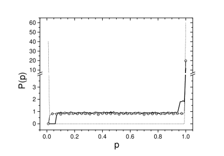
FIG. 1.: Probability density distributions obtained after $10^{4}$ steps (solid line), $2\times 10^{4}$steps (open circles) and $2\times 10^{6}$ steps (dash line), using Eq.(12), $2\eta N=1$, and $\mu=0.6$. the first distribution shows a rigid displacement to the right; the next ones show how the population is progressively polarized.

The intermediate stages in the gradient descent are also shown in Fig. 1. In the first few steps the (fast) uniform correction of $O(N)$ is seen to shift rigidly the initial distribution to one side with the aim of adjusting the value of $<p>$ to that of $\mu$. As a consequence, agents are piled up in one end while the other is completely cleared. Once the leading term in ${\cal C}$ is nearly canceled, the slow dynamics gradually gathers agents at both ends of the distribution producing minor fluctuations in the value of $<p>$. The density distribution $P(p)$ that is finally obtained is seen to correspond to a strongly polarized population thus reproducing the main feature of the equilibrium distributions obtained with the rules traditionally used in the GMG or the BAM.

The present approach yields a density distribution that displays the same polarization that is found in the GMG or in the BAM. It is remarkable that such a general qualitative agreement is found, although those frameworks differ deeply from the deterministic formulation. The conceptual difference between the two approaches lies in the special role played by the record of successes and failures that is kept in the BAM or GMG and that is completely absent in the present treatment. The usual rules of the GMG can thus be considered to correspond to a dynamics constrained by the (positive) balance of points that have been accumulated in the past instances of the game. There are other differences that deserve further discussion. These are related to the stochastic elements of the dynamics used in that framework which are absent from the present one. Within this approach, these can be assimilated to the effects of a finite temperature. We turn to this point in the next section.

IV Thermal fluctuations

The usual rules of the BAM or the GMG involve a stochastic updating of the attendance probabilities of each customer. When the account of points of the $i-$th player falls below zero a new value of $p_{i}$ is chosen at random from the interval $(p_{i}-\delta p/2,p_{i}+\delta p/2)$. This can be interpreted as a kind of thermal fluctuation in which $\delta p$ can be related to the temperature.

A few qualitative features support this. In equilibrium, the population is drastically polarized into those that consistently go to the bar (and therefore $p_{i}=1$) and those that do not go ($p_{i}=0$). A small fraction having $p_{i}$’s with intermediate values continuously migrate between both extreme strategies. This migration causes that the value of $<p>$ fluctuates around $\mu$. These random values of $<p>$ have a distribution that is sharply peaked at that value and has a width that is regulated by $\delta p$. In what regards the density distribution $P(p)$, a small value of $\delta p$ produces sharp peaks at $p=0$ and $p=1$ and $P(p)\sim 0$ for intermediate values. For larger values of $\delta p$ there is a larger fraction of players that migrate between $p=0$ and $p=1$ thus producing a rising in the “bottom” of the distribution $P(p)$.

The above qualitative arguments provide hints to introduce thermal fluctuations in the deterministic dynamics presented in the preceeding section and also about their relationship with $\delta p$ for the case of the GMG. However a singular situation occurs for $\delta p\rightarrow 0$ that is associated to an infinitely long relaxation process or when $\delta p>1$ in which this parameter loses its physical meaning of a being a probability.

Thermal-like fluctuations can formally be introduced following the same steps as the Langevin approach to describe a Brownian particle.In the present situation we start with the Eq. (9) for the motion of the average value $<p>$, and we add a stochastic term $L(t)$ that accounts for the random fluctuations

$$\frac{dW_{s}(t)}{dt}=-2\eta(N-1)W_{s}(t)-2\eta(\frac{1}{2}-\mu)+L(t)$$ (13)

We have added an index $s$ to $W(t)$ in Eq. (9) to stress the fact that this is the value of $W(t)$ in the presence of stochastic external fluctuations. The source of noise $L(t)$ can be taken to be the average of $N$ uncorrelated sources of random fluctuations affecting all the independent agents. One still has to specify a parameter related to the statistical properties of the distribution of the stochastic function $L(t)$. We will shortly prove that this is closely related to the temperature. As usual we assume:

$$\overline{L(t)} = 0$$ (14)

$$\overline{L(t)L(t^{\prime})} = \Gamma\delta(t-t^{\prime})$$ (15)

In Eqs. (14) and (15) and in all what follows $\overline{(\dots)}$ denotes an average over a suitable ensemble of replicas of the $N-$ agent system. The parameter $\Gamma$ is a constant that represents the mean square amplitude of instantaneous, uncorrelated perturbations. The stochastic differential equation (13) can explicitly be integrated. The result is

$$W_{s}(t)=W(t)+\mbox{e}^{-2\eta(N-1)t}\int_{0}^{t}\mbox{e}^{2\eta(N-1)\omega}L(\omega)d\omega$$ (16)

where $W(t)$ is the solution given in Eq(10) in which no fluctuations are present. If an average is made on both sides of Eq. (16), over a sub-ensemble of systems having the same initial conditions $W_{o}$ appearing in Eq. (10), one can immediately see that Eq. (14) implies that $\overline{W_{s}(t)}=W(t)$ and therefore the convergence of $<p>$ to $\mu$ (up to terms $O(1/N)$ is also insured within the stochastic dynamics. If the mean square fluctuations of $W_{s}(t)$ are calculated with the aid of Eq. (15), we get:

$$\overline{W_{s}^{2}(t)}=W^{2}(t)+\frac{\Gamma}{4\eta N}\quad\Bigl{[}1-\mbox{e}^{-4\eta Nt}\Bigr{]}\quad$$ (17)

The effect of the stochastic term in $W_{s}(t)$ produces a non vanishing value $\overline{W_{s}^{2}(\infty)}$. In ordinary statistical mechanics, the mean square fluctuations of the stationary solution of the velocity of Brownian particles is directly related to its average kinetic energy and can be set equal to $kT$. By analogy we formally define a temperature parameter $T$ that is independent from the size of the system, as the mean square fluctuations of $<p>$ in an equilibrium configuration, scaled by the number of agents of the system. Neglecting terms $O(1/N^{2})$ we obtain:

$$T\doteq N\overline{(<p>-\mu)^{2}}=\frac{\Gamma}{4\eta}$$ (18)

The parameter $\eta$ is a factor relating $T$ with the amplitude of the random fluctuations and plays a similar role than the Boltzmann constant.

Eq. (18) allows to write the ensemble average of the cost $\overline{{\cal C}}$ for an equilibrium configuration and for finite temperature. Up to the leading order in $N$ we obtain:

$$\overline{{\cal C}} = N^{2}\overline{(\mu-<p>)^{2}}+N\overline{(<p>-<p^{2}>)}$$ (19)

$$= N[T+\mu-\overline{<p^{2}>}]$$ (20)

$\overline{{\cal C}}$ is a positive, extensive magnitude which, in equilibrium, grows linearly with the size of the system and can therefore be taken to play the role of an internal energy.

The linear dependence of $\overline{{\cal C}}$ with the size of the system can be checked for the GMG. To do so we have calculated the cost using the definition of Eq.(4), with different number of agents. We first allowed the system to relax to the asymptotic equilibrium configuration and performed a suitable ensemble average over several replicas of the system. The linear dependence is shown in Fig. 2. The last iteration steps are used to estimate the dispersion of the numerical result and is shown with a pair of dotted lines. The slope of these lines change slightly with the parameter $\delta p$ of the GMG. This is due the relation between $T$ and $\delta p$ that we discuss later.

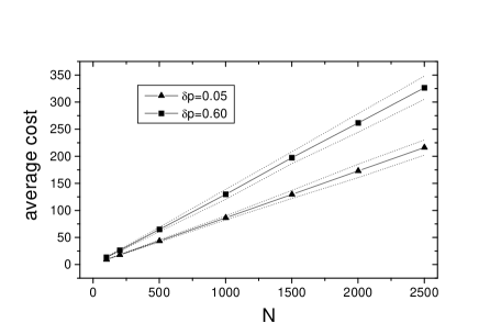
FIG. 2.: Linear dependence of ${\overline{\cal C}}$ as a function of $N$ for the GMG, $\mu=0.6$ and different values of $\delta p$

V Thermal relaxation

To include thermal fluctuations into a numerical treatment of the deterministic dynamics amounts only to introduce a random additive term in Eq.(12), namely:

$$p_{i}(t+1)=p_{i}(t)+\Delta(p_{i})+L_{\tau}^{(i)}(t)$$ (21)

where $L_{\tau}=\tau(1/2-r)$ and $r$ is a random number uniformly distributed in the interval $[0,1]$. This function represents the fluctuations produced on the $i$-th agent by a thermal bath. The temperature is defined by the second moment $\Gamma$ of the probability density of the $L_{\tau}^{(i)}(t)$.

The limit in which $L_{\tau}^{(i)}(t)$ has zero width (and therefore $\tau=0$) corresponds to the deterministic dynamics discussed in Sec. II. Larger values of $\tau$ are associated to fluctuations that may eventually override the updating amplitude $\Delta(p_{i})$ and tend to smear the distribution with two sharp $\delta$-functions, increasing the fraction of the population that have strategies $p_{i}\not=0$ or 1. (see Fig. 3$(a)$). If $\tau$ is further increased the polarization is progressively destroyed because the drift of the $p_{i}$’s towards 0 or 1 has to equilibrate against random shocks that prevent them to reach those limiting values.

FIG. 3.: (a) Probability density distribution obtained with the thermal dynamic of Eq.(21) for the values of $\tau$ that are shown in the inset. (b) Same distributions obtained with the stochastic dynamics of the GMG, for the values of $\delta p$ shown in the inset.

Given the stochastic dynamics of Eq.(21) together with the definition in Eq.(18) it is possible to calculate the value of $T$ in an equilibrium configuration, and relate $T$ with $\tau$. The parameter $\eta$ has to be chosen such that the relaxation of the deterministic dynamics is guaranteed i.e. when the time constant $\lambda=1/(2\eta N)$ introduced in Sect. 3 is $\lambda\sim 1$. In Fig. 4 we show that, as expected, $T\sim\tau^{2}$.

Eq.(18) allows also to calculate $T$ in any configuration reached through the stochastic dynamics of the GMG or the BAM. With this we can check two important features. The first is an estimation of the finite size corrections in the definition of $T$ given in Eq.(18), i.e. the regime in which $T$ is independent of the size of the system. The second outcome is to establish a quantitative relationship between $T$ and $\delta p$ that goes into the relaxation dynamics of the GMG.

We have calculated $W_{s}^{2}(t)$ for the GMG using several values of $\delta p$ and $N$. We have allowed $t$ to be large enough to reach equilibrium. We have then performed an ensemble average over several replicas of the system. The last steps have been used to gauge the dispersion of the numerical values. The results are shown in Fig.4$(b)$ where we plot $N\overline{W_{s}^{2}(\infty)}$ as a function of $\delta p$.

All the above mentioned features can be extracted from Fig. 4. Firstly finite size effects are clearly seen to affect only the smallest systems up to $N\sim 500$. Second the independence of $N\overline{W_{s}^{2}(\infty)}$ from the size of the system as assumed in the definition of Eq.(18) follows from the fact that the curves for $N\geq 500$ lump tightly together. In the third place a linear regression of all the curves establishes that $\delta p$ and $T$ have the same physical interpretations, and within the interval considered are nearly proportional to each other, namely $T=K\delta p$, with $K=(320\pm 20)10^{-4}$.

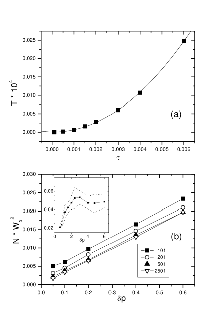
FIG. 4.: (a) Relationship between $\tau$ and $T$ as defined in Eq. (18). Solid squares correspond to the numerical calculation, while the line is the quadratic regression $10^{4}T=5.4310^{-5}-.114\tau+703.9\tau^{2}$, with $R^{2}=0.9999$. (b) linear dependence of the fluctuations $N\overline{W^{2}_{s}}$ with $\delta p<1$ for the GMG, and several values of $N$ (indicated in the figure). The upper inset shows that fluctuations saturate at a limiting value $\sim.05$ if the plot is extended for $\delta p>1$

The fact that $T$ and $\delta p$ are conceptually equivalent leads to extend the GMG simulations to higher values of $\delta p$. These values have seldom been explored [14] in the literature because this parameter measures the minor adjustments performed by the agents that try to find the “best” attendance probability. Large values of $\delta p$ could for instance correspond to irresolute or hesitating agents.

There are however important points that have to be considered. In the first place the value of $\delta p$ can not be taken arbitrarily large. This is so because it measures the uncertainty of the value of a probability. Values of $\delta p\ {\stackrel{{\scriptstyle>}}{{\sim}}}\ 1$ have therefore little physical meaning. In addition, if $\delta p$ is nevertheless extended to values higher than 1 by any plausible analytical extension (for instance using periodic or reflective boundary conditions), the fluctuations $\overline{W_{s}^{2}}$ for $\delta p>1$ are seen to saturate at an approximately constant value (see inset in Fig. 4$(b)$). These facts cause that the correspondence between $\delta p$ and $T$ necessarily breaks down.

A comparison of the probability density distributions $P(p)$ obtained with both approaches further supports this departure. In Fig. 3$(b)$ we show the equilibrium density distributions that are obtained with the stochastic, asynchronous updating rules of the GMG for two values of $\delta p$ (and $\mu=0.6$). It is seen that these diverge from those of Fig. 3$(a)$ that are obtained with the dynamics given in Eq.(21). Note however that there are noticeable ressemblances for small amplitude fluctuations. See for instance the distributions plotted in full line in Fig.3(b) and the one for $\tau=0.003$ in Fig.3(a).

As mentioned before, the origin of the departure between both dynamics can be found in the scoring of successes and failures that is used in the GMG, that is absent in the present approach. Some customers can be considered to be excluded from the updating dynamics as a consequence of their great accumulation of points. This, for instance, produces the large value of $P(p=1)$: many players that have accumulated a large positive account attending the bar do not change strategy. The scoring of each player works as a kind of “Maxwell Deamon” that classifies agents into different groups, endowing each one with a different updating rate.

The equilibrium configuration that is reached in the GMG therefore entails a distribution of updating rates in which some players are essentially frozen while others modify their attendance strategies frequently. This situation is completely different to the one obtained with the dynamics of Eq.(21) in which all agents undergo stochastic perturbations in every time step.

In order to show this we present in Fig. 5 some results of the GMG, in which we have used a large value of $\delta p$ ($\delta p=0.8$) and we have arbitrarily partitioned the ensemble of 1001 players into two sets. One of the sets gathers all players having at most 10 points the other contains all the rest. We have plotted their respective density distributions $P(p)$. The agents having less that 11 points are the ones that participate more strongly in the dynamics because undergo more frequent updatings.

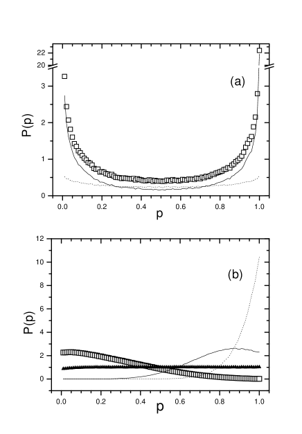
FIG. 5.: Partial probability density distributions of individual attendance strategies for the GMG for different subsets of players obtained for 1001 players, crowding level of 600/1001, and averages made over 2000 histories. (a) Asymptotic distributions. Subset of players with more than 10 accumulated points (full line) and with less than 11 points (dash line). The total probability density distribution is shown with empty boxes. (b) Density distributions at the end of the first 10 steps of the simulation. Players with 0 points (open boxes) have the greatest mobility, players with 5 and 10 points (full and dash lines respectively) have lower mobility. The total density distribution is shown in full triangles

The above comparison indicates that the GMG and the thermal relaxation dynamics of Eq.(21) strictly coincide only in the limit of $T\rightarrow 0$. However the strong qualitative resemblance of the results for $\delta p\leq.6$ allows to interpret $\delta p$, with these limitations, as equivalent to a thermal fluctuation.

The thermal interpretation of $\delta p$ has one interesting consequence. The most remarkable feature of the relaxation processes of the GMG performed with large $\delta p$ is that the high fluctuations prevents quenching (see Fig. 6). This allows to provide a new framework to the annealing procedure presented in Refs.[6] and [7] that resembles more closely the traditional protocol of Ref.[8].

The method presented in Ref.[6] requires an iterative procedure which involves a short evolution of the $N-$ agent system and the subsequent elimination of all points accumulated in the system. This is repeated until a moment in which the distribution $P(p)$ remains stationary. With the present interpretation of $\delta p$, a thermal annealing relaxation for the GMG can be performed for the cases in which $\mu$ is significantly different from 1/2. This new protocol can be assumed to take place in episodes. In the first episode, relaxation is allowed using a value of $\delta p$ that is large enough to insure that equilibrium is reached and quenching is prevented. The following episodes start from the equilibrium reached in the preceeding one, and a new relaxation process is allowed with a smaller value of $\delta p$ that is still large enough to avoid the appearance of quenching. The process continues until a lower bound of $\delta p$ is reached. Following this “cooling” protocol quenching never occurs, an absolute minimum of ${\cal C}$ is obtained and the population remains strongly polarized.

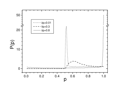
FIG. 6.: Asymptotic probability density distributions of individual attendance strategies for the GMG obtained with the values of $\delta p$ that are shown in the inset. Notice that for the highest value of $\delta p$ there is no quenching.

VI Conclusions

In the present paper we provide and alternative description of the dynamics of a system composed by many agents that play at the GMG. This is given in terms of the optimization of a single global magnitude, instead of doing it in terms independent actions of the $N$ agents. We do this by studying the effect of introducing a cost function ${\cal C}$ that is associated to the second moment of the probability distribution of the size of the attending parties.

We have proven that ${\cal C}$ has the relevant properties of an internal energy. In equilibrium, it is a positive extensive quantity that scales linearly with the number of agents $N$ and its minima correspond to equilibrium configurations with a highly polarized population, as found in the BAM or the GMG without quenching.

In addition, the deterministic dynamics that is derived from the descent along the gradient of ${\cal C}$ leads the system to configurations that have an equivalent polarization as that found with the traditional stochastic updating of the BAM or the GMG. This is a non trivial equivalence between two completely different organization schemes of the N-agent system. On the one hand the gradient descent gives rise to a set of coupled differential equations that represents a coordinated evolution of all the agents as would be the result of the action of a “central planner” of the whole system. On the other hand, within the GMG all the agents act independently from each other adjusting their attendance strategies with the purpose of optimizing their individual utilities. Even though the two relaxation mechanisms are very different, the final configurations of the system turn out to have equivalent features.

The definition of ${\cal C}$ in terms of the second moment of the probability distribution of attending parties is reminiscent of the many body Hamiltonian introduced in Ref.[13] to cast a version of the MG into the spin glass formalism. In the present case ${\cal C}$ can also be considered as a many body Hamiltonian with one- and two-body interactions in which the $N$ dynamic variables are the attendance probabilities $p_{i}$’s, with $i=1,2\dots N$.

The introduction of ${\cal C}$ and the associated relaxation process allows to define a temperature parameter through a Langevin-like approach. The value of $T$ remains associated to the ensemble average of the square of the fluctuations of the attendance, scaled by the number of agents. Its introduction in ${\cal C}$ provides the proof that this quantity, in thermal equilibrium, scales linearly with the size $N$ of the system and therefore qualifies as an extensive parameter.

On the other hand, in order to be an intensive parameter, $T$ should be independent of the size of the system. This has been checked numerically for the case of the GMG. However finite size effects in the definition of $T$ become negligible only for systems that are significantly larger than the minimal ones that already display the self organization features and that have spurred the popularity of the Minority Game.

Thermal fluctuations can be included in the dynamics that corresponds to the descent along the gradient of ${\cal C}$. The corresponding distributions $P(p)$ can readily be found and a comparison can be made of $T$ with $\delta p$ involved in the relaxation of the GMG or the BAM. A direct relationship can be established between both parameters but only in the limit of $\delta p\rightarrow 0$. We have also considered the dynamics of the GMG with moderately large values of $\delta p$ when still the divergence between the GMG and the thermal dynamics is not important. A stochastic updating that involves large values of $\delta p$ could be thought to be associated to irresolute or badly informed agents that correct their attendance probabilities performing significant changes in each correction.

The GMG relaxation for large values of $\delta p$ avoids quenching even for $\mu$ significantly different from 1/2. This fact, together with the thermal interpretation of $\delta p$ allows to cast the annealing procedure presented in Ref.[6] into the more traditional framework in which $T$ is progressively reduced in successive epochs. This “cooling” protocol could well be assimilated to a succession of learning episodes of the many agent system. In the first episodes in which agents have little “experience” and the information about the past is scarce, all agents perform large amplitude - even random - corrections. In the last episodes of the relaxation process, as there is a richer information about the past history of the system the agents perform finer corrections, the fluctuations are smaller and the cost paid by a wrong attendance are also smaller.

The fact that on the one hand an extensive magnitude can be defined playing the role of an internal energy, and that on the other, a microscopic definition of the temperature can be made, opens the way to a the full thermodynamic description of a system of N-agent performing a GMG. This amount to introduce a Gibbs distribution defined as $\Phi({\cal C})=e^{-{\cal C}/T}/Z$, where $Z$ stands for the partition function. All thermodynamic functions should follow from this.

E.B. has been partially supported by CONICET of Argentina, PICT-PMT0051;H.C. and R.P. were partially supported by EC grant ARG/b7-3011/94/27, Contract 931005 AR.

REFERENCES

- [1] Amer. Econ. Assoc. Papers Proc. 84, 406 (1994)
- [2] D. Challet, Y.C. Zhang, Physica A246, 407 (1997); Physica A256, 514 (1998)
- [3] R. Savit, R. Manuca, R. Riolo, Phys. Rev. Lett. 82, 2203 (1999)
- [4] A. Cavagna, Phys. Rev. E59, R3783 (1999)
- [5] N.F. Johnson, P.M. Hui, R. Jonson, T.S. Lo, Phys. Rev. Lett. 82, 3360 (1999)
- [6] E.Burgos, H. Ceva and R.Perazzo. Physica A294, 539 (2001)
- [7] E.Burgos, H. Ceva and R.Perazzo. Phys RevE, in press
- [8] S. Kirkpatrick, C.D. Gelatt and P.P. Vecchi, Science 220, 671 (1983)
- [9] In Ref.[7] the average of Eq.(4) is defined as instead of as we do here. We prefer the present notation because, as we prove later, this quantity, in equilibrium, scales linearly with the size of the system as corresponds to an extensive quantity.
- [10] N.F. Johnson, D.J.T. Leonard, P.M. Hui, T.S. Lo, cond-mat /9905939 v2. See also: N.F. Johnson, P.M. Hui, Dafang Zeng, C.W. Tai, Physica A269, 493 (1999)
- [11] E. Burgos, H.Ceva, Physica A284, 489 (2000)
- [12] A.Goldberg Genetic Algorithms in Search, Optimization, and Machine Learning, Addison - Wesley (1989).
- [13] D. Challet, M. Marsili Phys. Rev. E60, R6271 (1999)
- [14] H.Ceva, Physica A277, 496 (2000)