Abstract

We describe some field theoretic methods for studying quantum spin systems in one dimension. These include the nonlinear $\sigma$-model approach which is particularly useful for large values of the spin, the idea of Luttinger liquids and bosonization which are more useful for small values of spin such as spin-$1/2$, and the technique of low-energy effective Hamiltonians which can be useful if the system under consideration is perturbatively close to an exactly solvable model. We apply these techniques to similar spin models, such as spin chains with dimerization and frustration, and spin ladders in the presence of a magnetic field. This comparative study illustrates the relative strengths of the different methods.

1 Introduction

One-dimensional and quasi-one-dimensional quantum spin systems have been studied extensively in recent years for several reasons. Many such systems have been realized experimentally, and a variety of theoretical techniques, both analytical and numerical, are available to study the relevant models. Due to large quantum fluctuations in low dimensions, such systems often have unusual properties such as a gap between a singlet ground state and the excited nonsinglet states; this leads to a magnetic susceptibility which vanishes exponentially at low temperatures. Perhaps the most famous example of this is the Haldane gap which was predicted theoretically in integer spin Heisenberg antiferromagnetic chains [1], and then observed experimentally in a spin-$1$ system $Ni(C_{2}H_{8}N_{2})_{2}NO_{2}(ClO_{4})$ [2]. Other examples include the spin ladder systems in which a small number of one-dimensional spin-$1/2$ chains interact amongst each other [3]. It has been observed that if the number of chains is even, i.e., if each rung of the ladder (which is the unit cell for the system) contains an even number of spin-$1/2$ sites, then the system effectively behaves like an integer spin chain with a gap in the low-energy spectrum. Some two-chain ladders which show a gap are $(VO)_{2}P_{2}O_{7}$ [4], $SrCu_{2}O_{3}$ [5] and $Cu_{2}(C_{5}H_{12}N_{2})_{2}Cl_{4}$ [6]. Conversely, a three-chain ladder which effectively behaves like a half-odd-integer spin chain and does not exhibit a gap is $Sr_{2}Cu_{3}O_{5}$ [5]. A related observation is that some quasi-one-dimensional systems such as $CuGeO_{3}$ spontaneously dimerize below a spin-Peierls transition temperature [7]; then the unit cell contains two spin-$1/2$ sites and the system is gapped. Another interesting class of systems are the alternating spin chains such as bimetallic molecular magnets. An example is $NiCu(pbaOH)(H_{2}O)_{3}\cdot 2H_{2}O$ in which spin-$1$’s ($Ni^{2+}$) and spin-$1/2$’s ($Cu^{2+}$) alternate. The ground state of these systems have a nonzero total spin $S_{0}$. It turns out that there is a gap to states with spin greater than $S_{0}$, but no gap to states with spin less than $S_{0}$.

The results for gaps quoted above are all in the absence of an external magnetic field. The situation becomes even more interesting in the presence of a magnetic field [8]. Then it is possible for an integer spin chain to be gapless and a half-odd-integer spin chain to show a gap above the ground state for appropriate values of the field [9, 10, 11, 12, 13]. This has been demonstrated in several models using a variety of methods such as exact diagonalization of small systems, bosonization and conformal field theory [14, 15], and perturbation theory [16]. In particular, it has been shown that the magnetization of some systems can exhibit plateaus at certain nonzero values for some finite ranges of the magnetic field.

The plan of this paper is as follows. In Sec. 2, we discuss the low-energy properties of the dimerized and frustrated antiferromagnetic spin chain. In Secs. 3 and 4, we present some field theoretic methods which can be used for studying spin chains and ladders with or without an external magnetic field [17]. These methods rely on the idea that the low-energy and long-wavelength modes of a system (i.e., wavelengths much longer than the lattice spacing $a$ if the system is defined on a lattice at the microscopic level) can often be described by a continuum field theory. In Sec. 3, we discuss the nonlinear $\sigma$-model approach, while in Sec. 4, we discuss the concepts of Tomonaga-Luttinger liquids and bosonization. In Sec. 5, we discuss the low-energy effective Hamiltonian approach and show how it can be combined with bosonization to gain an understanding of the magnetic properties of one-dimensional spin systems.

2 Spin Chain with Dimerization and Frustration

Experimental studies of some of the quasi-one-dimensional spin systems have shown that besides the nearest neighbor antiferromagnetic exchange, there also exists a second neighbor exchange $J_{2}$ of the same sign and comparable magnitude. Such a second neighbor interaction has the effect of frustrating the spin alignment favored by the nearest neighbor interaction. Therefore, a realistic study of one-dimensional systems requires a model with both frustration ($J_{2}$) and dimerization (governed by a parameter $\delta$).

The Hamiltonian for the frustrated and dimerized antiferromagnetic spin chain can be written as

$$H~{}=~{}\sum_{i}~{}[~{}1~{}-~{}(-1)^{i}~{}\delta~{}]~{}{\vec{S}}_{i}\cdot{\vec{S}}_{i+1}~{}+~{}J_{2}~{}\sum_{i}~{}{\vec{S}}_{i}\cdot{\vec{S}}_{i+2}~{},$$ (1)

where the limits of the summation depend on the boundary condition (open or periodic). (We have set the average nearest neighbor interaction $J_{1}$ to be equal to $1$ for convenience). The interactions are schematically shown in Fig. 1. The region of interest is defined by $J_{2}~{}\geq 0$ and $0\leq\delta\leq 1$.

Figure 1: Schematic picture of the spin chain described by Eq. (1).

The ground state properties of the Hamiltonian (1) have been studied at some representative points in the $J_{2}-\delta$ plane using the density-matrix renormalization group (DMRG) method [18]. The phase diagrams obtained for spin-$1/2$ and spin-$1$ chains are shown in Figs. 2 and 3 [19]. We use the word ‘phase’ only for convenience to distinguish between regions with different modulations of the two-spin correlation function as discussed later. Our model actually has no phase transition even at zero temperature.

For the spin-$1/2$ chain [20, 21], the system is found to be gapless on the line $A$ which runs from $J_{2}=0$ to $J_{2c}=0.241$ for $\delta=0$; see Fig. 2. The model is gapped everywhere else in the $J_{2}-\delta$ plane. There is a disorder line $B$ given by $2J_{2}+\delta=1$ on which the exact ground state of the model is given by a product of singlets formed by the nearest-neighbor spins which are joined by the stronger bonds ($1+\delta$); this is called the Shastry-Sutherland line [22], and it ends at the Majumdar-Ghosh point $(J_{2}=0.5,\delta=0)$. The correlation length $\xi$ goes through a minimum on $B$. Finally, the peak in the structure factor $S(q)$ is at $q_{max}=\pi$ to the left of $B$ (called region I), decreases from $\pi$ to $\pi/2$ as one goes from $B$ up to the line $C$ (region II), and is at $q_{max}=\pi/2$ to the right of $C$ (region III).

Figure 2: Ground state phase diagram of the spin-$1/2$ chain in the $J_{2}-\delta$ plane.

In the spin-$1$ case (Fig. 3), the phase diagram is more complex. There is a solid line marked $A$ which runs from $(0,0.25)$ to about $(0.22\pm 0.02,0.20\pm 0.02)$ shown by a cross. To within numerical accuracy, the gap is zero on this line and the correlation length $\xi$ is as large as the system size $N$. The rest of the ‘phase’ diagram is gapped. However the gapped portion can be divided into different regions characterized by other interesting features. On the dotted lines marked $B$, the gap is finite. Although $\xi$ goes through a maximum when we cross $B$ in going from region II to region I or from region III to region IV, its value is much smaller than $N$. There is a dashed line $C$ extending from $(0.65,0.05)$ to about $(0.73,0)$ on which the gap appears to be zero (to numerical accuracy), and $\xi$ is very large but not as large as $N$. In regions II and III, the ground state for an open chain has a four-fold degeneracy (consisting of $S=0$ and $S=1$), whereas it is nondegenerate in regions I and IV with $S=0$. The regions II and III, where the ground state of an open chain is four-fold degenerate, can be identified with the Haldane phase. The regions I and IV correspond to the non-Haldane singlet phase. Regions I and IV are separated by the disorder line $D$ given by $2J_{2}+\delta=1$, while regions II and III are separated by line $E$. The lines $B$, $D$ and $E$ seem to meet in a small region V where the ground state of the model is numerically very difficult to find.

Figure 3: Ground state phase diagram of the spin-$1$ chain.

As can be seen from Fig. 1, setting $\delta=1$ results in a two-chain ladder where the interchain coupling is $2$ and the intrachain coupling is $J_{2}$. We can hold $J_{2}$ fixed and vary the interchain coupling $J$. Numerical studies show that for spin-$1/2$, the system is gapped for any nonzero value of $J$, although the gap vanishes linearly as $J\rightarrow 0$; this can be shown using bosonization. On the other hand, the spin-$1$ chain has a finite value of the gap for any value of $J$ [19].

3 Nonlinear $\sigma$-model

The nonlinear $\sigma$-model (NLSM) analysis of spin chains with the inclusion of $J_{2}~{}$ and $\delta$ proceeds as follows [23]. We first do a classical analysis in the $S\rightarrow\infty$ limit to find the ground state configuration of the spins. Let us make the ansatz that the ground state is a coplanar configuration of the spins with the energy per spin being equal to

$$e_{0}~{}=~{}S^{2}~{}\left[{1\over 2}~{}(1+\delta)\cos\theta_{1}~{}+~{}{1\over 2}~{}(1-\delta)\cos\theta_{2}~{}+~{}J_{2}\cos(\theta_{1}+\theta_{2})\right]~{},$$ (2)

where $\theta_{1}$ is the angle between the spins ${\vec{S}}_{2i}$ and ${\vec{S}}_{2i+1}$ and $\theta_{2}$ is the angle between the spins ${\vec{S}}_{2i}$ and ${\vec{S}}_{2i-1}$. Minimization of the classical energy with respect to the $\theta_{i}~{}$ yields the following three phases.

(i) Neel: This phase has $\theta_{1}=\theta_{2}=\pi$; hence all the spins point along the same line and they go as $\uparrow\downarrow\uparrow\downarrow$ along the chain. This phase is stable for $1-\delta^{2}>4J_{2}$.

(ii) Spiral: Here, the angles $\theta_{1}$ and $\theta_{2}$ are given by

$$\cos\theta_{1} = -{1\over{1+\delta}}~{}{\left[~{}{{1-\delta^{2}}\over{4J_{2}}}~{}+~{}{\delta\over{1+\delta^{2}}}~{}4J_{2}~{}\right]}$$

$${\rm and}\quad\cos\theta_{2} = -{1\over{1-\delta}}~{}{\left[~{}{{1-\delta^{2}}\over{4J_{2}}}~{}-~{}{\delta\over{1-\delta^{2}}}~{}{4J_{2}}~{}\right]},$$ (3)

where $\pi/2<\theta_{1}<\pi$ and $0<\theta_{2}<\theta_{1}$. Thus the spins lie on a plane. This phase is stable for $1-\delta^{2}<4J_{2}<(1-\delta^{2})/\delta$.

(iii) Colinear: This phase (which needs both dimerization and frustration) is defined to have $\theta_{1}=\pi$ and $\theta_{2}=0$; hence all the spins point along the same line and they go as $\uparrow\uparrow\downarrow\downarrow$ along the chain. It is stable for $(1-\delta^{2})/\delta<4J_{2}$.

These phases along with their boundaries are depicted in Fig. 4. Thus even in the classical limit $S\rightarrow\infty$, the system has a rich ground state ‘phase diagram’.

Figure 4: Classical ground state phase diagram of the spin chain with frustration and dimerization.

We can go to the next order in $1/S$, and study the spin wave spectrum about the ground state in each of the phases. The main results are as follows. In the Neel phase, we find two zero modes, i.e., modes for which the energy $\omega_{k}$ vanishes linearly at certain values of the momentum $k$, with the slope $d\omega_{k}/dk$ at those points being called the velocity. The two modes are found to have the same velocity in this phase. In the spiral phase, we have three zero modes, two with the same velocity describing out-of-plane fluctuations, and one with a higher velocity describing in-plane fluctuations. In the colinear phase, we get two zero modes with equal velocities just as in the Neel phase. The three phases also differ in the behavior of the spin-spin correlation function $S(q)=\sum_{n}\langle{\vec{S}}_{0}\cdot{\vec{S}}_{n}\rangle\exp(-iqn)$ in the classical limit. $S(q)$ is peaked at $q=(\theta_{1}+\theta_{2})/2$, i.e., at $q=\pi$ in the Neel phase, at $\pi/2<q<\pi$ in the spiral phase and at $q=\pi/2$ in the colinear phase. Even for $S=1/2$ and $1$, DMRG studies have seen this feature of $S(q)$ in the Neel and spiral phases [19].

Figure 5: Classical configuration of the spins in the Neel phase.

We now derive a NLSM field theory which can describe the low-energy and long-wavelength excitations. In the Neel phase, this is given by a $O(3)$ NLSM with a topological term [1, 15]. The field variable is a unit vector $\vec{\phi}$ which is defined as follows. The classical ground state in the Neel phase has a unit cell, labeled by an integer $n$, with two sites labeled as $1n$ and $2n$ respectively; see Fig. 5. We define linear combinations of the two spins as

$${\vec{\phi}}_{n}~{} = ~{}\frac{{\vec{S}}_{1n}~{}-~{}{\vec{S}}_{2n}}{2S}~{},$$

$${\vec{l}}_{n}~{} = ~{}\frac{{\vec{S}}_{1n}~{}+~{}{\vec{S}}_{2n}}{2a}~{}.$$ (4)

Here $a$ is the lattice spacing; hence, the size of each unit cell is $2a$. Note that

$${\vec{l}}_{n}~{}\cdot~{}{\vec{\phi}}_{n}~{} = ~{}0~{},$$

$${\vec{\phi}}_{n}^{2}~{} = ~{}1~{}+~{}\frac{1}{S}~{}-~{}\frac{a^{2}{\vec{l}}_{n}^{2}}{S^{2}}~{},$$ (5)

so that ${\vec{\phi}}_{n}$ becomes an unit vector in the large $S$ limit. These fields satisfy the commutation relations

$$[~{}l_{ma}~{},~{}\phi_{nb}~{}]~{}=~{}\frac{i}{2a}~{}\delta_{mn}~{}\sum_{c}~{}\epsilon_{abc}~{}\phi_{nc}~{},$$ (6)

where $m,n$ are unit cell labels, $a,b,c$ denote the components $x,y,z$, and $\epsilon_{abc}$ is the completely antisymmetric tensor with $\epsilon_{xyz}=1$. This means that we can write ${\vec{l}}_{n}={\vec{\phi}}_{n}\times{\vec{\Pi}}_{n}$, where the vector $\vec{\Pi}$ is canonically conjugate to $\vec{\phi}$, i.e.,

$$[~{}\phi_{ma}~{},~{}\Pi_{nb}~{}]~{}=~{}\frac{i}{2a}~{}\delta_{mn}~{}\delta_{ab}~{}.$$ (7)

We now go to the continuum limit by introducing a spatial coordinate $x$ which is equal to $2na$ at the location of the $n^{\rm th}$ unit cell. Summations get replaced by integrals, i.e., $\sum_{n}\rightarrow\int dx/(2a)$. The commutation relation (7) then takes the form

$$[~{}\phi_{a}(x)~{},~{}\Pi_{b}(y)~{}]~{}=~{}i~{}\delta(x-y)~{}\delta_{ab}~{}.$$ (8)

We note that $\dot{\vec{\phi}}$ and ${\vec{\phi}}^{\prime}$ are orthogonal to $\vec{\phi}$ because $\vec{\phi}$ is an unit vector. We will see below that both $\vec{l}$ and $\vec{\Pi}$ are given by first-order space-time derivatives of $\phi$. In the low-energy and long-wavelength limit, the dominant terms in the Hamiltonian will be those which have second-order derivatives of $\vec{\phi}$, and therefore first-order derivatives of $\vec{l}$. To find this Hamiltonian, we rewrite (1) in terms of $\vec{\phi}$ and $\vec{l}$, and Taylor expand these fields to the necessary order, i.e.,

$${\vec{\phi}}_{n+1}~{} = ~{}{\vec{\phi}}(x)~{}+~{}2a{\vec{\phi}}^{\prime}(x)~{}+~{}2a^{2}{\vec{\phi}}^{\prime\prime}~{}+~{}\ldots~{},$$

$${\vec{l}}_{n+1}~{} = ~{}{\vec{l}}(x)~{}+~{}2a{\vec{l}}^{\prime}(x)~{}+~{}\ldots~{},$$ (9)

where $x=2na$. We then use the constraints in (5) and do some integration by parts (throwing away boundary terms at $x=\pm\infty$) to obtain the continuum Hamiltonian

$$H~{}=~{}\int~{}dx~{}[~{}\frac{cg^{2}}{2}~{}({\vec{l}}+\frac{\theta}{4\pi}{\vec{\phi}}^{\prime})^{2}~{}+~{}\frac{c}{2g^{2}}~{}{\vec{\phi}}^{\prime 2}~{}]~{},$$ (10)

where

$$c~{} = ~{}2aS{\sqrt{1-4J_{2}-\delta^{2}}}~{},$$

$$g^{2}~{} = ~{}\frac{2}{S{\sqrt{1-4J_{2}-\delta^{2}}}}~{},$$

$${\rm and}\quad\theta~{} = ~{}2\pi S(1-\delta)~{}.$$ (11)

By expanding (10) to second order in small fluctuations around, say, ${\vec{\phi}}=(0,0,1)$, we find an energy-momentum dispersion relation of the ‘massless relativistic’ form $\omega=c|k|$; thus $c$ is the spin wave velocity. Similarly, by expanding (10) to fourth and higher orders in small fluctuations, we find that $g^{2}$ is the coupling constant governing the strength of the interactions between the spin waves.

One can show that the Hamiltonian (10) follows from the Lagrangian density

$${\cal L}~{}=~{}{1\over{2cg^{2}}}~{}{\dot{\vec{\phi}}}^{2}~{}-~{}{c\over{2g^{2}}}~{}{\vec{\phi}}^{\prime 2}~{}+~{}{\theta\over{4\pi}}~{}{\vec{\phi}}\cdot{\vec{\phi}}^{\prime}\times{\dot{\vec{\phi}}}~{},$$ (12)

(Incidentally, one can derive the canonically conjugate momentum $\vec{\Pi}$ and then the angular momentum $\vec{l}$ from (12),

$${\vec{\Pi}}~{} = ~{}\frac{1}{cg^{2}}~{}{\dot{\vec{\phi}}}~{}+~{}\frac{\theta}{4\pi}~{}{\vec{\phi}}\times{\vec{\phi}}^{\prime}~{},$$

$${\vec{\l}}~{} = ~{}{\vec{\phi}}\times{\vec{\Pi}}~{}=~{}\frac{1}{cg^{2}}~{}{\vec{\phi}}\times\dot{\vec{\phi}}~{}-~{}\frac{\theta}{4\pi}~{}{\vec{\phi}}^{\prime}~{},$$ (13)

thereby verifying that $\vec{l}$ and $\vec{\Pi}$ only contain first-order derivatives of $\vec{\phi}$ as stated above). From (12), we see that $\theta$ is the coefficient of a topological term, because the integral of this term is an integer which defines the winding number of a field configuration ${\vec{\phi}}(x,t)$). For $\theta=\pi$ mod $2\pi$ and $g$ less than a critical value $g_{c}$, it is known that the system is gapless and is described by a conformal field theory with an $SU(2)$ symmetry [15, 24]. For any other value of $\theta$, the system is gapped, and the gap is of order $\Delta E\sim\exp(-2\pi/g^{2})$. For $J_{2}=\delta=0$, one therefore expects that integer spin chains should have a gap of the order $\exp(-\pi S)$ (note that this goes to zero rapidly as $S\rightarrow\infty$, so that there is no difference between integer and half-odd-integer spin chains in the classical limit), while half-integer spin chains should be gapless. For the two-spin equal-time correlation function, this means that $<{\vec{S}}_{0}\cdot{\vec{S}}_{n}>$ should decay as a power-law $(-1)^{n}/|n|$ as $|n|\rightarrow\infty$ for half-odd-integer spin chains, and exponentially as $(-1)^{n}\exp(-n/\xi)$ for integer spin chains, where the correlation length $\xi\sim c/\Delta E$. All this is known to be true even for small values of $S$ like $1/2$ (analytically) and $1$ (numerically) although the field theory is only derived for large $S$. In the presence of dimerization, one expects a gapless system at certain special values of $\delta$. For $S=1$, the special value is predicted to be $\delta_{c}=0.5$. We see that the existence of a gapless point is correctly predicted by the NLSM. However, according to the DMRG results, $\delta_{c}~{}$ is at $0.25$ for $J_{2}=0$ [25] and it decreases with $J_{2}~{}$ as shown in Fig. 3; this differs from the NLSM results in (11) according to which $\theta$ should be independent of $J_{2}$. These deviations from field theory are probably due to higher order corrections in $1/S$ which have not been studied analytically so far.

In the spiral phase of the $J_{2}-\delta$ model, it is necessary to use a different NLSM which is known for $\delta=0$ [26, 27]. The field variable is now an $SO(3)$ matrix $\underline{R}$. The Lagrangian density is

$${\cal L}~{}=~{}{1\over{2cg^{2}}}~{}{\rm tr}~{}\Bigl{(}~{}{\dot{\underline{R}}^{T}}{\dot{\underline{R}}}~{}P_{0}~{}\Bigr{)}~{}-~{}{c\over{2g^{2}}}~{}{\rm tr}~{}\Bigl{(}~{}{\underline{R}}^{\prime T}{\underline{R}}^{\prime}~{}P_{1}~{}\Bigr{)},$$ (14)

where $c=S(1+y){\sqrt{1-y^{2}}}/y$, $g^{2}=2{\sqrt{(1+y)/(1-y)}}/S$ with $1/y=4J_{2}~{}$, and $P_{0}~{}$ and $P_{1}~{}$ are diagonal matrices with diagonal elements $(1,1,2y(1-y)/(2y^{2}-2y+1))$ and $(1,1,0)$ respectively. Note that there is no topological term; indeed, no such term is possible since $\Pi_{2}(SO(3))=0$ unlike $\Pi_{2}(S^{2})=Z$ for the $O(3)$ NLSM in the Neel phase. Hence there is no apparent difference between integer and half-integer spin chains in the spiral phase. A one-loop renormalization group [26] and large $N$ analysis [27] indicate that the system should have a gap for all values of $J_{2}~{}$ and $S$, and that there is no reason for a particularly small gap at any special value of $J_{2}~{}$. The ‘gapless’ point found numerically at $J_{2}=0.73$ for spin-$1$ is therefore a surprise.

Finally, in the colinear phase of the $J_{2}-\delta$ model, the NLSM is known for $\delta=1$, i.e., for the spin ladder. The Lagrangian is the same as in (12), but with $c=4aS{\sqrt{J_{2}(J_{2}+1)}}$, $g^{2}={\sqrt{1+1/J_{2}}}/S$ and $\theta=0$. There is no topological term for any value of $S$, and the model is therefore gapped.

The field theories for general $\delta$ in both the spiral and colinear phases are still not known. Although the results are qualitatively expected to be similar to the $\delta=0$ case in the spiral phase and the $\delta=1$ case in the colinear phase, quantitative features such as the dependence of the gap on the coupling strengths require the explicit form of the field theory.

The NLSMs derived above can be expected to be accurate only for large values of the spin $S$. It is interesting to note that the ‘phase’ boundary between Neel and spiral for spin-$1$ is closer to the the classical ($S\rightarrow\infty$) boundary $4J_{2}=1-\delta^{2}$ than for spin-$1/2$. For instance, the cross-over from Neel to spiral occurs, for $\delta=0$, at $J_{2}=0.5$ for spin-$1/2$, at $0.39$ for spin-$1$, and at $0.25$ classically.

To summarize, we have studied a two-parameter ‘phase’ diagram for the ground state of isotropic antiferromagnetic spin-$1/2$ and spin-$1$ chains using the NLSM approach, and have compared the results with those obtained numerically. We find that the spin-$1$ diagram is considerably more complex than the corresponding spin-$1/2$ chain with surprising features like a ‘gapless’ point inside the spiral ‘phase’; this point could be close to a critical point discussed earlier in the literature [24, 28]. It would be interesting to establish this more definitively.

Our results show that frustrated spin chains with small values of $S$ exhibit some features not anticipated from large $S$ field theories like the NLSMs. The NLSMs also leave many questions unanswered. For instance, the $O(3)$ NLSM which is applicable in the Neel phase does not tell us the exponent of the gap which opens up as one moves away from $\theta=\pi$ (for $g<g_{c}$) or as we go across $g=g_{c}$ (for $\theta=\pi$). To address these questions, we have to use the more powerful technique of bosonization.

The NLSM approach can also be used to study spin chains in the presence of a magnetic field. Consider adding a Zeeman term to the Hamiltonian in (1), i.e.,

$$H~{}=~{}\sum_{i}~{}[~{}1~{}-~{}(-1)^{i}~{}\delta~{}]~{}{\vec{S}}_{i}\cdot{\vec{S}}_{i+1}~{}+~{}J_{2}~{}\sum_{i}~{}{\vec{S}}_{i}\cdot{\vec{S}}_{i+2}~{}-~{}\sum_{i}~{}{\vec{B}}\cdot{\vec{S}}_{i}~{},$$ (15)

where $\vec{B}$ denotes the magnetic field. In the region $1-\delta^{2}>4J_{2}$, the classical ground state of this Hamiltonian is given by a coplanar configuration in which the spins ${\vec{S}}_{2i}$ and ${\vec{S}}_{2i+1}$ lie at angles $\pm~{}\alpha$ respectively with respect to the magnetic field, so that the angle between the spins ${\vec{S}}_{2i}$ and ${\vec{S}}_{2i+1}$ is $2\alpha$. Minimization of the energy fixes the angle $\alpha$ to be

$$\alpha~{}=~{}\cos^{-1}\Bigl{(}~{}\frac{|{\vec{B}}|}{4S}~{}\Bigr{)}~{}.$$ (16)

(We are assuming that $|{\vec{B}}|<4S$, otherwise all the spins will align with the magnetic field and $\alpha$ will be zero). We now define

$${\vec{\phi}}_{n}~{} = ~{}\frac{{\vec{S}}_{1n}~{}-~{}{\vec{S}}_{2n}}{2S\sin\alpha}~{},$$

$${\vec{l}}_{n}~{} = ~{}\frac{{\vec{S}}_{1n}~{}+~{}{\vec{S}}_{2n}}{2a}~{}.$$ (17)

Note that the definition of $\vec{\phi}$ is slightly different from the one in (4) in order to ensure that $\vec{\phi}$ is an unit vector. However, $\vec{l}$ is orthogonal to and has the same commutation relations with $\vec{\phi}$ as before. We can now go to the continuum limit and derive the Hamiltonian

$$H~{}=~{}\int~{}dx~{}[~{}\frac{cg^{2}}{2}~{}({\vec{l}}+\frac{\theta}{4\pi}{\vec{\phi}}^{\prime})^{2}~{}+~{}\frac{c}{2g^{2}}~{}{\vec{\phi}}^{\prime 2}-{\vec{B}}\cdot{\vec{l}}~{}]~{},$$ (18)

where

$$c~{} = ~{}2aS\sin\alpha~{}{\sqrt{1-4J_{2}-\delta^{2}}}~{},$$

$$g^{2}~{} = ~{}\frac{2}{S\sin\alpha{\sqrt{1-4J_{2}-\delta^{2}}}}~{},$$

$${\rm and}\quad\theta~{} = ~{}2\pi S\sin\alpha~{}(1-\delta)~{}.$$ (19)

We can show that this follows from the Lagrangian density

$${\cal L}~{} = ~{}{1\over{2cg^{2}}}~{}[~{}{\vec{\phi}}\times\dot{\vec{\phi}}+{\vec{B}}-({\vec{B}}\cdot{\vec{\phi}}){\vec{\phi}}~{}]^{2}~{}-~{}{c\over{2g^{2}}}~{}{\vec{\phi}}^{\prime 2}~{}+~{}{\theta\over{4\pi}}~{}{\vec{\phi}}\cdot{\vec{\phi}}^{\prime}\times{\dot{\vec{\phi}}}~{},$$ (20)

$$= ~{}{1\over{2cg^{2}}}~{}[~{}{\dot{\vec{\phi}}}^{2}+2{\vec{B}}\times{\vec{\phi}}\cdot{\dot{\vec{\phi}}}+{\vec{B}}^{2}-({\vec{B}}\cdot{\vec{\phi}})^{2}~{}]~{}-~{}{c\over{2g^{2}}}~{}{\vec{\phi}}^{\prime 2}~{}+~{}{\theta\over{4\pi}}~{}{\vec{\phi}}\cdot{\vec{\phi}}^{\prime}\times{\dot{\vec{\phi}}}~{}.$$

We see from this that

$${\vec{l}}~{}=~{}{\vec{\phi}}\times{\vec{\Pi}}~{}=~{}\frac{1}{cg^{2}}~{}[~{}{\vec{\phi}}\times\dot{\vec{\phi}}~{}+~{}{\vec{B}}~{}-~{}({\vec{B}}\cdot{\vec{\phi}}){\vec{\phi}}~{}]~{}-~{}\frac{\theta}{4\pi}~{}{\vec{\phi}}^{\prime}~{}.$$ (21)

Since $cg^{2}=4a$ and ${\vec{B}}\cdot{\vec{\phi}}=0$ in the classical ground state, we see that $\vec{l}$ is equal to ${\vec{B}}/(4a)$ plus small fluctuations; this agrees with its definition in (17) and the classical configuration of the spins. One can now analyse the field theory governed by (20) using the renormalization group and other methods. We refer the reader to [29] for further details.

4 Bosonization

A very useful method for studying spin systems in one dimension is the technique of bosonization. Before describing this method, let us briefly present some background information. Further details can be found in Refs. [14, 15, 30, 31].

In one dimension, a great variety of interacting quantum systems (both fermionic and bosonic) is described by the Tomonaga-Luttinger liquid (TLL) theory. Typically, a TLL describes quantum systems which are translation invariant and gapless, i.e., the excitation energy above the ground state is zero in the limit of the system size $L\rightarrow\infty$. A TLL differs in three significant ways from the well-known Fermi liquid theory which describes many fermionic systems in two and three dimensions. First, all the low-energy excitations in a TLL have the character of sound modes which are bosonic and have a linear dispersion relation between the energy and the momentum (with the constant of proportionality being the sound velocity $v$). Even if the underlying theory is fermionic, the low-energy excitations are given by particle-hole pairs which are bosonic. The properties of a TLL are governed by two important parameters, namely, an interaction parameter $K$ (noninteracting systems have $K=1$) and the velocity $v$. Secondly, the one-particle momentum distribution function $n(k)$ for fermions, which is obtained by Fourier transforming the fermion Green’s function

$$G(x,t)~{}=~{}<0|T\psi(x,t)\psi^{\dagger}(0,0)|0>$$ (22)

and computing the residue of its pole in the complex $\omega$ plane as a function of $k$, has no discontinuity at the Fermi surface $k=k_{F}$ for a TLL. Instead, it has a cusp there of the form

$$n(k)~{}=~{}n(k_{F})~{}+~{}{\rm const.}~{}{\rm sign}(k-k_{F})~{}|k-k_{F}|^{(1-K)^{2}/2K}~{}.$$ (23)

On the other hand, in a Fermi liquid, $n(k)$ has a finite discontinuity at the Fermi surface; see Fig. 6. Finally, correlation functions in a TLL typically decay at large distances as power-laws which depend on $K$, unlike the correlation functions of a Fermi liquid where the power-laws are universal.

Figure 6: One-particle momentum distribution function for (a) an interacting Fermi liquid, and (b) a Tomonaga-Luttinger liquid.

Let us be more specific about the nature of the low-energy excitations in a one-dimensional system of interacting fermions. Assume that we have a system of length $L$ with periodic boundary conditions; the translation invariance and the finite length make the one-particle momenta discrete. Suppose that the system has $N_{0}$ particles with a ground state energy $E_{0}(N_{0})$ and a ground state momentum $P_{0}=0$. We will be interested in the thermodynamic limit $N_{0},L\rightarrow\infty$ keeping the particle density $\rho_{0}=N_{0}/L$ fixed. If we could switch off the interactions, the fermions would have two Fermi points, at $k=\pm k_{F}$ respectively, with all states with momenta lying between the two points being occupied. (See Fig. 7 for a typical picture of the momentum states of a lattice model without interactions). Even in the presence of interactions, it turns out that the low-lying excitations consist of two pieces [32],

(i) a set of bosonic excitations each of which can have either positive momentum $q$ or negative momentum $-q$ with an energy $\epsilon_{q}=vq$, where $0<q<<k_{F}$ and $v$ is the sound velocity, and

(ii) a certain number of particles $N_{R}$ and $N_{L}$ added to the right and left Fermi points respectively, where $N_{R},N_{L}<<N_{0}$. Note that $N_{R}$ and $N_{L}$ can be positive, negative or zero.

The quasiparticle excitations in (i) have an infinite number of degrees of freedom (in the thermodynamic limit), and they determine properties such as specific heat and susceptibility to various perturbations. The particle excitations in (ii) only have two degrees of freedom and therefore play no role in the thermodynamic properties. The Hamiltonian and momentum operators for a one-dimensional system (which may have interactions) have the general form

$$H~{}= E_{0}(N_{0})~{}+~{}\sum_{q>0}~{}vq~{}{[}~{}{\tilde{b}}_{R,q}^{\dagger}{\tilde{b}}_{R,q}~{}+~{}{\tilde{b}}_{L,q}^{\dagger}{\tilde{b}}_{L,q}~{}{]}~{}$$

$$+~{}\mu(N_{R}+N_{L})~{}+~{}\frac{\pi v}{2LK}(N_{R}+N_{L})^{2}~{}+~{}\frac{\pi vK}{2L}~{}(N_{R}-N_{L})^{2}~{},$$

$$P~{}= \sum_{q>0}~{}q~{}{[}~{}{\tilde{b}}_{R,q}^{\dagger}{\tilde{b}}_{R,q}~{}-~{}{\tilde{b}}_{L,q}^{\dagger}{\tilde{b}}_{L,q}~{}{]}~{}+~{}[~{}k_{F}~{}+~{}\frac{\pi}{L}(N_{R}+N_{L})~{}]~{}(N_{R}-N_{L})~{},$$ (24)

where $q$ is the momentum of the low-energy bosonic excitations created and annihilated by ${\tilde{b}}_{q}^{\dagger}$ and ${\tilde{b}}_{q}$, $K$ is a positive dimensionless number, and $\mu$ is the chemical potential of the system. We will see later that $v$ and $K$ are the two important parameters which determine all the low-energy properties of a system. Their values generally depend on both the strength of the interactions and the density. If the fermions are noninteracting, we have

$$v~{}=~{}v_{F}\quad{\rm and}\quad K~{}=~{}1~{}.$$ (25)

Note that one can numerically find the values of $v$ and $K$ by varying $N_{R}$ and $N_{L}$ and studying the $1/L$ dependence of energy and momentum of finite size systems.

The technique of bosonization (combined with conformal field theory) is very useful for analytically studying a TLL [14, 15, 30, 31]. This technique consists of mapping bosonic operators into fermionic ones, and then using whichever set of operators is easier to compute with.

To begin, let us consider a fermion with both right- and left-moving components. We introduce a chirality label $\nu$, such that $\nu=R$ and $L$ refer to right- and left-moving particles respectively. Sometimes we will use the numerical values $\nu=1$ and $-1$ for $R$ and $L$; this will be clear from the context. Then the second quantized Fermi fields are given by

$$\psi_{\nu}(x)~{} = ~{}\frac{1}{\sqrt{L}}~{}\sum_{k=-\infty}^{\infty}~{}c_{\nu,k}~{}e^{i\nu kx}~{},$$

$$k~{} = ~{}\frac{2\pi}{L}~{}n_{k}~{},$$ (26)

where $n_{k}=0,\pm 1,\pm 2,...$, and

$$\{c_{\nu,k},c_{\nu^{\prime},k^{\prime}}\}~{} = ~{}0~{},$$

$$\{c_{\nu,k},c_{\nu^{\prime},k^{\prime}}^{\dagger}\}~{} = ~{}\delta_{\nu\nu^{\prime}}~{}\delta_{kk^{\prime}}~{}.$$ (27)

Next we define bosonic operators

$$b_{\nu,q}^{\dagger}~{} = ~{}\frac{1}{\sqrt{n}_{q}}~{}\sum_{k=-\infty}^{\infty}~{}c_{\nu,k+q}^{\dagger}c_{\nu,k}~{},$$

$$b_{\nu,q}~{} = ~{}\frac{1}{\sqrt{n}_{q}}~{}\sum_{k=-\infty}^{\infty}~{}c_{\nu,k-q}^{\dagger}c_{\nu,k}~{}.$$ (28)

Note that $b_{R,q}^{\dagger}$ and $b_{L,q}^{\dagger}$ create excitations with momenta $q$ and $-q$ respectively, where the label $q$ is always taken to be positive. We can show that

$${[}b_{\nu,q},b_{\nu^{\prime},q^{\prime}}{]}~{}=~{}0~{},\quad{\rm and}\quad{[}b_{\nu,q},b_{\nu^{\prime},q^{\prime}}^{\dagger}{]}~{}=~{}\delta_{\nu\nu^{\prime}}~{}\delta_{qq^{\prime}}~{}.$$ (29)

The vacuum state of the system is defined to be the state $|0>$ which is annihilated by the operators $c_{\nu,k}$ for $k\geq 0$ and $c_{\nu,k}^{\dagger}$ for $k<0$, and therefore by $b_{\nu,q}$ for all $q$.

Let us define the chiral bosonic fields

$$\phi_{\nu}(x)~{}=~{}\frac{i\nu}{2{\sqrt{\pi}}}~{}\sum_{q>0}~{}\frac{1}{\sqrt{n}_{q}}~{}[~{}b_{\nu,q}~{}e^{i\nu qx-\alpha q/2}~{}-~{}b_{\nu,q}^{\dagger}~{}e^{-i\nu qx-\alpha q/2}~{}]~{}-~{}\frac{\sqrt{\pi}x}{L}~{}{\hat{N}}_{\nu}~{},$$ (30)

where the length parameter $\alpha$ is a cut-off which is required to ensure that the contribution from high-momentum modes do not produce divergences when computing correlation functions. The fields in (30) satisfy

$${[}\phi_{\nu}(x),\phi_{\nu^{\prime}}(x){]}~{}=~{}-\frac{i\nu}{4}~{}\delta_{\nu\nu^{\prime}}~{}{\rm sign}~{}(x-x^{\prime})$$ (31)

in the limit $\alpha\rightarrow 0$. It is useful to define two fields dual to each other

$$\phi(x)~{} = ~{}\phi_{R}(x)~{}+~{}\phi_{L}(x)~{},$$

$$\theta(x)~{} = ~{}-~{}\phi_{R}(x)~{}+~{}\phi_{L}(x)~{}.$$ (32)

Then $[\phi(x),\phi(x^{\prime})]=[\theta(x),\theta(x^{\prime})]=0$, while

$${[}\phi(x),\theta(x^{\prime}){]}~{}=~{}\frac{i}{2}~{}{\rm sign}~{}(x-x^{\prime})~{}.$$ (33)

Now it can be shown that the fermionic and bosonic operators discussed above are related to each other as

$$\psi_{R}~{} = ~{}\frac{1}{\sqrt{2\pi\alpha}}~{}\eta_{R}~{}e^{-i2{\sqrt{\pi}}\phi_{R}}~{},$$

$$\psi_{L}~{} = ~{}\frac{1}{\sqrt{2\pi\alpha}}~{}\eta_{L}~{}e^{i2{\sqrt{\pi}}\phi_{L}}~{},$$ (34)

in the sense that they produce the same state when they act on the vacuum state $|0>$, and they have the same correlation functions. The unitary operators $\eta_{R}$ and $\eta_{L}$ are called Klein factors, and they are essential to ensure that the fermionic fields given in Eq. (34) anticommute at two different spatial points $x$ and $y$.

The densities of the right- and left-moving fermions are given by $\rho_{R}=\psi_{R}^{\dagger}\psi_{R}$ and $\rho_{L}=\psi_{L}^{\dagger}\psi_{L}$. The total fermionic density and current are given by

$$\rho~{}-~{}\rho_{0}~{} = ~{}\rho_{R}+\rho_{L}~{}=~{}-~{}\frac{1}{\sqrt{\pi}}~{}\frac{\partial\phi}{\partial x}~{},$$

$$j~{} = ~{}v_{F}~{}(\rho_{R}-\rho_{L})~{}=~{}\frac{v_{F}}{\sqrt{\pi}}~{}\frac{\partial\theta}{\partial x}~{},$$ (35)

where $\rho_{0}$ is the background density (fluctuations around this density are described by the fields $\psi$ or $\phi$), and the velocity $v_{F}$ will be introduced below.

Let us now introduce a Hamiltonian. We assume a linear dispersion relation $\epsilon_{\nu,k}=v_{F}k$ for the fermions. The noninteracting Hamiltonian then takes the form

$$H_{0} = v_{F}\sum_{k=-\infty}^{\infty}~{}k~{}{[}~{}c_{R,k}^{\dagger}c_{R,k}~{}+~{}c_{L,k}^{\dagger}c_{L,k}~{}{]}~{}+~{}\frac{\pi v_{F}}{L}({\hat{N}}_{R}^{2}+{\hat{N}}_{L}^{2})$$ (36)

$$= -v_{F}\int_{0}^{L}dx~{}[\psi_{R}^{\dagger}(x)i\partial_{x}\psi_{R}(x)~{}-~{}\psi_{L}^{\dagger}(x)i\partial_{x}\psi_{L}(x)]~{}+~{}\frac{\pi v_{F}}{L}({\hat{N}}_{R}^{2}+{\hat{N}}_{L}^{2})$$

in the fermionic language, and

$$H_{0}~{} = ~{}v_{F}~{}\sum_{q>0}~{}q~{}(~{}b_{R,q}^{\dagger}b_{R,q}~{}+~{}b_{L,q}^{\dagger}b_{L,q}~{})~{}+~{}\frac{\pi v_{F}}{L}({\hat{N}}_{R}^{2}+{\hat{N}}_{L}^{2})$$ (37)

$$= ~{}v_{F}~{}\int_{0}^{L}~{}dx~{}[~{}(\partial_{x}\phi_{R})^{2}~{}+~{}(\partial_{x}\phi_{L})^{2}~{}]$$

$$= ~{}\frac{v_{F}}{2}~{}\int_{0}^{L}~{}dx~{}[~{}(\partial_{x}\phi)^{2}~{}+~{}(\partial_{x}\theta)^{2}~{}]$$

in the bosonic language.

We now study the effects of four-fermi interactions. Let us consider an interaction of the form

$$V~{}=~{}\frac{1}{2}~{}\int_{0}^{L}~{}dx~{}[~{}2g_{2}~{}\rho_{R}(x)\rho_{L}(x)~{}+~{}g_{4}~{}(~{}\rho_{R}^{2}(x)~{}+~{}\rho_{L}^{2}(x)~{})~{}]~{}.$$ (38)

Physically, we may expect an interaction such as $g\rho^{2}/2$, so that $g_{2}=g_{4}=g$. However, it is instructive to allow $g_{2}$ to differ from $g_{4}$ to see what happens. Also, we will not assume anything about the signs of $g_{2}$ and $g_{4}$. In the fermionic language, the interaction takes the form

$$V=\frac{1}{2L}\sum_{k_{1},k_{2},k_{3}=-\infty}^{\infty} [ 2g_{2}c_{R,k_{1}+k_{3}}^{\dagger}c_{R,k_{1}}c_{L,k_{2}+k_{3}}^{\dagger}c_{L,k_{2}}$$

$$~{}+g_{4}(c_{R,k_{1}+k_{3}}^{\dagger}c_{R,k_{1}}c_{R,k_{2}-k_{3}}^{\dagger}c_{R,k_{2}}+c_{L,k_{1}+k_{3}}^{\dagger}c_{L,k_{1}}c_{L,k_{2}-k_{3}}^{\dagger}c_{L,k_{2}})]~{}.$$

From this expression we see that $g_{2}$ corresponds to a two-particle scattering involving both chiralities; in this model, we can call it either forward scattering or backward scattering since there is no way to distinguish between the two processes in the absence of some other quantum number such as spin. The $g_{4}$ term corresponds to a scattering between two fermions with the same chirality, and therefore describes a forward scattering process.

The quartic interaction in Eq. (LABEL:int) seems very difficult to analyze. However we will now see that it is easily solvable in the bosonic language; indeed this is one of the main motivations behind bosonization. The bosonic expression for the total Hamiltonian $H=H_{0}+V$ is found to be

$$H = \sum_{q>0}~{}q{[}v_{F}(b_{R,q}^{\dagger}b_{R,q}+b_{L,q}^{\dagger}b_{L,q})+\frac{g_{2}}{2\pi}(b_{R,q}^{\dagger}b_{L,q}^{\dagger}+b_{R,q}b_{L,q})+\frac{g_{4}}{2\pi}(b_{R,q}^{\dagger}b_{R,q}+b_{L,q}^{\dagger}b_{L,q}){]}$$ (40)

$$~{}~{}+\frac{\pi v_{F}}{L}(~{}{\hat{N}}_{R}^{2}+{\hat{N}}_{L}^{2}~{})+~{}\frac{g_{2}}{L}~{}{\hat{N}}_{R}{\hat{N}}_{L}~{}+~{}\frac{g_{4}}{2L}(~{}{\hat{N}}_{R}^{2}+{\hat{N}}_{L}^{2}~{}).$$

The $g_{4}$ term only renormalizes the velocity. The $g_{2}$ term can then be rediagonalized by a Bogoliubov transformation. We first define two parameters

$$v~{} = ~{}\Bigl{[}~{}(~{}v_{F}+\frac{g_{4}}{2\pi}-\frac{g_{2}}{2\pi}~{})~{}(~{}v_{F}+\frac{g_{4}}{2\pi}+\frac{g_{2}}{2\pi}~{})~{}\Bigr{]}^{1/2}~{},$$

$$K~{} = ~{}\Bigl{[}~{}(~{}v_{F}+\frac{g_{4}}{2\pi}-\frac{g_{2}}{2\pi}~{})~{}/~{}(~{}v_{F}+\frac{g_{4}}{2\pi}+\frac{g_{2}}{2\pi}~{})~{}\Bigr{]}^{1/2}~{}.$$ (41)

Note that $K<1$ if $g_{2}$ is positive (repulsive interaction), and $>1$ if $g_{2}$ is negative (attractive interaction). [If $g_{2}$ is so large that $v_{F}+g_{4}/(2\pi)-g_{2}/(2\pi)<0$, then our analysis breaks down. The system does not remain a Luttinger liquid in that case, and is likely to go into a different phase such as a state with charge density order]. The Bogoliubov transformation then takes the form

$${\tilde{b}}_{R,q}~{} = ~{}\frac{b_{R,q}~{}+~{}\gamma~{}b_{L,q}^{\dagger}}{\sqrt{1-\gamma^{2}}}~{},$$

$${\tilde{b}}_{L,q}~{} = ~{}\frac{b_{L,q}~{}+~{}\gamma~{}b_{R,q}^{\dagger}}{\sqrt{1-\gamma^{2}}}~{},$$

$${\rm where}\quad\gamma~{} = ~{}\frac{1-K}{1+K}~{},$$ (42)

for each value of the momentum $q$. The Hamiltonian is then given by the quadratic expression

$$H~{}=~{} \sum_{q>0}~{}vq~{}{[}~{}{\tilde{b}}_{R,q}^{\dagger}{\tilde{b}}_{R,q}~{}+~{}{\tilde{b}}_{L,q}^{\dagger}{\tilde{b}}_{L,q}~{}{]}$$ (43)

$$+~{}\frac{\pi v}{2L}~{}[~{}\frac{1}{K}~{}({\hat{N}}_{R}+{\hat{N}}_{L})^{2}~{}+~{}K~{}({\hat{N}}_{R}-{\hat{N}}_{L})^{2}~{}]~{}.$$

Equivalently,

$$H~{}=~{}\frac{1}{2}~{}\int_{0}^{L}~{}dx~{}[~{}vK\Pi^{2}~{}+~{}\frac{v}{K}~{}(\partial_{x}\phi)^{2}~{}]~{}.$$ (44)

The old and new fields are related as

$$\phi_{R}~{} = ~{}\frac{(1+K)~{}{\tilde{\phi}}_{R}~{}-~{}(1-K)~{}{\tilde{\phi}}_{L}}{2{\sqrt{K}}}~{},$$

$$\phi_{L}~{} = ~{}\frac{(1+K)~{}{\tilde{\phi}}_{L}~{}-~{}(1-K)~{}{\tilde{\phi}}_{R}}{2{\sqrt{K}}}~{},$$

$$\phi~{} = ~{}{\sqrt{K}}~{}{\tilde{\phi}}\quad{\rm and}\quad\theta~{}=~{}\frac{1}{\sqrt{K}}~{}{\tilde{\theta}}~{}.$$ (45)

Note the important fact that the vacuum changes as a result of the interaction; the new vacuum $|{\tilde{0}}\rangle$ is the state annihilated by the operators ${\tilde{b}}_{\nu,q}$. Since the various correlation functions must be calculated in this new vacuum, they will depend on the interaction through the parameters $v$ and $K$. In particular, we will see below that the power-laws of the correlation functions are governed by $K$.

Given the various Hamiltonians, it is easy to guess the forms of the corresponding Lagrangians. For the noninteracting theory ($g_{2}=g_{4}=0$), the Lagrangian density describes a massless Dirac fermion,

$${\cal L}~{}=~{}i\psi_{R}^{\dagger}(\partial_{t}+v_{F}\partial_{x})\psi_{R}~{}+~{}i\psi_{L}^{\dagger}(\partial_{t}-v_{F}\partial_{x})\psi_{L}$$ (46)

in the fermionic language, and a massless real scalar field,

$${\cal L}~{}=~{}\frac{1}{2v_{F}}~{}(\partial_{t}\phi)^{2}~{}-~{}\frac{v_{F}}{2}~{}(\partial_{x}\phi)^{2}$$ (47)

in the bosonic language. For the interacting theory in Eq. (44), we find from Eq. (45) that

$${\cal L}~{}=~{}\frac{1}{2vK}~{}(\partial_{t}\phi)^{2}~{}-~{}\frac{v}{2K}~{}(\partial_{x}\phi)^{2}~{}=~{}\frac{1}{2v}~{}(\partial_{t}{\tilde{\phi}})^{2}~{}-~{}\frac{v}{2}~{}(\partial_{x}{\tilde{\phi}})^{2}~{}.$$ (48)

Although the dispersion relation is generally not linear for all the modes of a realistic system, it often happens that the low-energy and long-wavelength modes (and therefore the low-temperature properties) can be described by a TLL. For a fermionic system in one dimension, these modes are usually the ones lying close to the two Fermi points with momenta $\pm k_{F}$ respectively; see Fig. 7. Although the fermionic field $\psi$ generally has components with all possible momenta, one can define right- and left-moving fields $\psi_{R}$ and $\psi_{L}$ which vary slowly on the scale length $a$,

$$\psi(x,t)~{}=~{}\psi_{R}(x,t)~{}e^{ik_{F}x}~{}+~{}\psi_{L}(x,t)~{}e^{-ik_{F}x}~{}.$$ (49)

Quantities such as the density generally contain terms which vary slowly as well as terms varying rapidly on the scale of $a$,

$$\rho-\rho_{0}~{} = ~{}\psi^{\dagger}\psi~{}=~{}\psi_{R}^{\dagger}\psi_{R}~{}+~{}\psi_{L}^{\dagger}\psi_{L}~{}+~{}e^{-i2k_{F}x}~{}\psi_{R}^{\dagger}\psi_{L}~{}+~{}e^{i2k_{F}x}~{}\psi_{L}^{\dagger}\psi_{R}$$ (50)

$$= ~{}-~{}\frac{1}{\sqrt{\pi}}~{}\frac{\partial\phi}{\partial x}~{}+~{}\frac{1}{2\pi\alpha}~{}{[}\eta_{R}^{\dagger}\eta_{L}e^{i(2{\sqrt{\pi}}\phi-2k_{F}x)}~{}+~{}\eta_{L}^{\dagger}\eta_{R}e^{-i(2{\sqrt{\pi}}\phi-2k_{F}x)}~{}{]}.$$

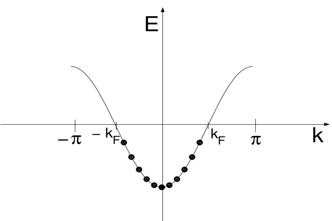
Figure 7: Picture of the ground state of a one-dimensional system of noninteracting fermions on a lattice. Filled circles denote occupied states lying below the Fermi energy $E_{F}=0$.

One can now compute various correlation functions in the bosonic language. Consider an operator of the exponential form

$$O_{m,n}~{}=~{}e^{i2{\sqrt{\pi}}(m\phi+n\theta)}~{}.$$ (51)

(Such an operator can arise from a product of several $\psi$’s and $\psi^{\dagger}$’s if we ignore the Klein factors; then Eq. (34) implies that $m\pm n$ must take integer values). We then find the following result for the two-point correlation function at space-time separations which are much larger than the microscopic lattice spacing $a$,

$$\langle{\tilde{0}}|~{}TO_{m,n}(x,t)O_{m^{\prime},n^{\prime}}^{\dagger}(0,0)~{}|{\tilde{0}}\rangle$$

$$\sim\delta_{mm^{\prime}}\delta_{nn^{\prime}}\frac{\alpha^{2(m^{2}K+n^{2}/K)}}{(vt-x-i\alpha{\rm sign}(t))^{(m{\sqrt{K}}-n/{\sqrt{K}})^{2}}(vt+x-i\alpha{\rm sign}(t))^{(m{\sqrt{K}}+n/{\sqrt{K}})^{2}}}~{}.$$

(52)

Note that the correlation function decays as a power-law, and the power depends on the interaction parameter $K$. In the language of the renormalization group, the scaling dimension of $O_{m,n}$ is given by

$$d_{O}~{}=~{}m^{2}K~{}+~{}\frac{n^{2}}{K}~{}.$$ (53)

We can now discuss a spin chain from the point of view of bosonization. To be specific, let us consider a spin-$1/2$ chain described by the anisotropic Hamiltonian

$$H~{}=~{}\sum_{i=1}^{N}~{}[~{}\frac{J}{2}~{}(S_{i}^{+}S_{i+1}^{-}+S_{i}^{-}S_{i+1}^{+})~{}+~{}J\Delta S_{i}^{z}S_{i+1}^{z}~{}-~{}hS_{i}^{z}~{}]~{},$$ (54)

where the interactions are only between nearest neighbor spins, and $J>0$. $S_{i}^{+}=S_{i}^{x}+iS_{i}^{y}$ and $S_{i}^{-}=S_{i}^{x}-iS_{i}^{y}$ are the spin raising and lowering operators, and $h$ denotes a magnetic field. Note that the model has a $U(1)$ invariance, namely, rotations about the $S^{z}$ axis. When $\Delta=1$ and $h=0$, the $U(1)$ invariance is enhanced to an $SU(2)$ invariance, because at this point the model can be written simply as $H=J\sum_{i}{\vec{S}_{i}}\cdot{\vec{S}_{i+1}}$.

Eq. (54) is the well-studied $XXZ$ spin-$1/2$ chain in a longitudinal magnetic field. It can be exactly solved using the Bethe ansatz, and a lot of information can then be obtained using conformal field theory [10, 32]. The following results are relevant for us. The model is gapless for a certain range of values of $\Delta$ and $h/J$. For instance, this is true if $-1<\Delta\leq 1$ and $h=0$; then the two-spin equal-time correlations have oscillatory pieces which decay asymptotically as

$$\langle S_{0}^{+}S_{n}^{-}\rangle~{} \sim ~{}\frac{(-1)^{n}}{|n|^{\eta}}~{},$$

$$\langle S_{0}^{z}S_{n}^{z}\rangle~{} \sim ~{}\frac{(-1)^{n}}{|n|^{1/\eta}}~{},$$

$${\rm where}\quad\eta~{} = ~{}\frac{1}{2}~{}+~{}\frac{1}{\pi}~{}\sin^{-1}~{}(\Delta)~{}.$$ (55)

For $\Delta>1$ and $h=0$, the system is gapped; there are two degenerate ground states which have a period of two sites consistent with the condition (68). Thus the invariance of the Hamiltonian under a translation by one site is spontaneously broken in the ground states. This is particularly obvious for $\Delta\rightarrow\infty$ where the two ground states are $+-+-\cdots$ and $-+-+\cdots$. The two-spin correlations decay exponentially for $\Delta>1$ and $h=0$. Finally, the system is gapped for $h/J>1+\Delta$ with all sites having $S_{z}=1/2$ in the ground state, and for $h/J<-1-\Delta$ with all sites having $S_{z}=-1/2$.

However, it is not easy to compute explicit correlation functions using the Bethe ansatz. We will therefore use bosonization to study the model in (54).

We first use the Jordan-Wigner transformation to map the spin model to a model of spinless fermions. We map an $\uparrow$ spin or a $\downarrow$ spin at any site to the presence or absence of a fermion at that site. We introduce a fermion annihilation operator $\psi_{i}$ at each site, and write the spin at the site as

$$S_{i}^{z} = \psi_{i}^{\dagger}\psi_{i}-1/2=n_{i}-1/2$$

$$S_{i}^{-} = (-1)^{i}~{}\psi_{i}e^{i\pi\sum_{j}n_{j}}~{},$$ (56)

where the sum runs from one boundary of the chain up to the $(i-1)^{\rm th}$ site (we assume an open boundary condition here for convenience), $n_{i}=0$ or $1$ is the fermion occupation number at site $i$, and the expression for $S_{i}^{+}$ is obtained by taking the hermitian conjugate of $S_{i}^{-}$, The string factor in the definition of $S_{i}^{-}$ is added in order to ensure the correct statistics for different sites; the fermion operators at different sites anticommute, whereas the spin operators commute.

We now find that

$$H~{}=~{}-~{}~{}\sum_{i}~{}[~{}\frac{J}{2}~{}(\psi_{i}^{\dagger}\psi_{i+1}+h.c.)~{}+~{}J\Delta~{}(n_{i}-1/2)(n_{i+1}-1/2)~{}-~{}h~{}(n_{i}-1/2)~{}]~{}.$$ (57)

We see that the spin-flip operators $S_{i}^{\pm}$ lead to hopping terms in the fermion Hamiltonian, whereas the $S_{i}^{z}S_{i+1}^{z}$ term leads to an interaction between fermions on adjacent sites.

Let us first consider the noninteracting case given by $\Delta=0$. By Fourier transforming the fermions, $\psi_{k}=\sum_{j}\psi_{j}e^{-ikja}/\sqrt{N}$, where $a$ is the lattice spacing and the momentum $k$ lies in the first Brillouin zone $-\pi/a<k\leq\pi/a$, we find that the Hamiltonian is given by

$$H~{}=~{}\sum_{k}~{}\omega_{k}~{}\psi_{k}^{\dagger}\psi_{k}~{},$$ (58)

where

$$\omega_{k}~{}=~{}-J~{}\cos(ka)~{}-~{}h~{}.$$ (59)

The noninteracting ground state is the one in which all the single-particle states with $\omega_{k}<0$ are occupied, and all the states with $\omega_{k}>0$ are empty. If we set the magnetic field $h=0$, the magnetization per site $m\equiv\sum_{i}S_{i}^{z}/N$ will be zero in the ground state; equivalently, in the fermionic language, the ground state is precisely half-filled. Thus, for $m=0$, the Fermi points ($\omega_{k}=0$) lie at $ka=\pm\pi/2\equiv k_{F}a$. Let us now add the magnetic field term. In the fermionic language, this is equivalent to adding a chemical potential term (which couples to $n_{i}$ or $S_{i}^{z}$). In that case, the ground state no longer has $m=0$ and the fermion model is no longer half-filled. The Fermi points are then given by $\pm k_{F}$, where

$$k_{F}a~{}=~{}\pi~{}(m~{}+~{}\frac{1}{2})~{}.$$ (60)

It turns out that this relation between $k_{F}$ (which governs the oscillations in the correlation functions as discussed below) and the magnetization $m$ continues to hold even if we turn on the interaction $J\Delta$, although the simple picture of the ground state (with states filled below some energy and empty above some energy) no longer holds in that case.

In the linearized approximation, the modes near the two Fermi points have the velocities $\partial\omega_{k}/\partial k=\pm v$, where $v$ is some function of $J$, $\Delta$ and $h$. Next, we introduce the slowly varying fermionic fields $\psi_{R}$ and $\psi_{L}$ as indicated above; these are functions of a coordinate $x$ which must be an integer multiple of $a$. Now we bosonize these fields. The spin fields can be written in terms of either the fermionic or the bosonic fields. For instance, $S^{z}$ is given by the fermion density as in Eq. (56) which then has a bosonized form given in Eq. (50). Similarly,

$$S^{+}(x,t)~{} = ~{}(-1)^{x/a}~{}[\psi_{R}^{\dagger}(x,t)e^{-ik_{F}x/a}+\psi_{L}^{\dagger}(x,t)e^{ik_{F}x/a}]~{}\times$$ (61)

$$~{}~{}~{}~{}~{}~{}~{}~{}~{}~{}~{}~{}[e^{i\pi\int_{-\infty}^{x}dx^{\prime}(\psi^{\dagger}(x^{\prime},t)\psi(x^{\prime},t)+1/2a)}+h.c.]~{},$$

where $(-1)^{x/a}=\pm 1$ since $x/a$ is an integer. This can now be written entirely in the bosonic language; the term in the exponential is given by

$$\int_{-\infty}^{x}dx^{\prime}\psi^{\dagger}(x^{\prime},t)\psi(x^{\prime},t)=-~{}{1\over\sqrt{\pi}}\int_{-\infty}^{x}dx^{\prime}\partial_{x^{\prime}}\phi~{}=~{}-~{}{1\over\sqrt{\pi}}~{}[\phi_{R}(x,t)+\phi_{L}(x,t)]~{},$$ (62)

where we have ignored the contribution from the lower limit at $x^{\prime}=-\infty$.

We can now use this bosonic expressions to compute the various two-spin correlation functions $G^{ab}(x,t)\equiv<0|TS^{a}(x,t)S^{b}(0,0)|0>$. We find that

$$G^{zz}(x,t) = m^{2}~{}+~{}c_{1}\Bigl{[}{1\over(x+vt)^{2}}+{1\over(x-vt)^{2}}\Bigr{]}+c_{2}\frac{\cos(2k_{F}x)}{(x^{2}-v^{2}t^{2})^{K}}~{},$$

$$G^{+-}(x,t)+G^{-+}(x,t) = c_{3}\frac{(-1)^{x/a}}{(x^{2}-v^{2}t^{2})^{1/4K}}$$

$$+c_{4}\frac{(-1)^{x/a}~{}\cos(2k_{F}x)}{(x^{2}-v^{2}t^{2})^{({\frac{1}{2{\sqrt{K}}}-{\sqrt{K}}})^{2}}}\Bigl{[}{1\over(x-vt)^{2}}+{1\over(x+vt)^{2}}\Bigr{]}~{},$$

where $c_{1},...,c_{4}$ are some constants. The Luttinger parameters $K$ and $v$ are functions of $\Delta$ and $h/J$ (or $m$). [The exact dependence can be found from the web site given in Ref. [10]; this contains a calculator which finds the values of $R=1/{\sqrt{4\pi K}}$ and $h/J$ if one inputs the values of $M=2m$ and $\Delta$]. For $h=0$, $K$ is given by the analytical expression

$${1\over K}~{}=~{}1~{}+~{}{2\over\pi}\sin^{-1}(\Delta)~{}.$$ (64)

Note that at the $SU(2)$ invariant point $\Delta=1$ and $h=0$, we have $K=1/2$, and the two correlations $G^{zz}$ and $G^{+-}$ have the same forms.

In addition to providing a convenient way of computing correlation functions, bosonization also allows us to study the effects of small perturbations which may take the system away from a TLL. For instance, a physically important perturbation is a dimerizing term

$$V~{}=~{}\delta\sum_{i}~{}(-1)^{i}~{}[~{}\frac{J}{2}~{}(S_{i}^{+}S_{i+1}^{-}+S_{i}^{-}S_{i+1}^{+})~{}+~{}J\Delta S_{i}^{z}S_{i+1}^{z}~{}]~{},$$ (65)

where $\delta$ is the strength of the perturbation. Upon bosonizing, we find that the scaling dimension of this term is $K$. Hence it is relevant if $K<2$; in that case, it produces an energy gap in the system which scales with $\delta$ as

$$\Delta E~{}\sim~{}\delta^{1/(2-K)}~{}.$$ (66)

For the isotropic case $\Delta=1$, we have $K=1/2$ and the gap scales as $\Delta E\sim\delta^{2/3}$. [This is the exponent of the gap which appears as we vary $\delta$ to move away from the gapless line $(0\leq J_{2}\leq J_{2c},\delta=0)$ for spin-$1/2$ in Fig. 2 or the line A for spin-$1$ in Fig. 3]. This phenomenon occurs in spin-Peierls systems such as $CuGeO_{3}$; below a transition temperature $T_{sp}$, they go into a dimerized phase which has a gap.

Another interesting perturbation occurs when the frustration parameter $J_{2}$ crosses the critical value $J_{2c}=0.241$ for $\delta=0$ in the spin-$1/2$ chain; see Fig. 2. This turns out to be a marginal perturbation, and it produces a gap which has an essential singularity of the form $\Delta E\sim\exp[-{\rm const.}/(J_{2}-J_{2c})]$ [33]. Because of this form, it is very hard to numerically measure the gap if $J_{2}$ is close to $J_{2c}$.

Finally, when two isotropic spin-$1/2$ chains (with the spin variables in the two chains being denoted by ${\vec{S}}^{(1)}_{n}$ and ${\vec{S}}^{(2)}_{n}$) are coupled together with a weak interchain coupling

$$V~{}=~{}J^{\prime}~{}\sum_{n}~{}{\vec{S}}^{(1)}_{n}\cdot{\vec{S}}^{(2)}_{n}~{},$$ (67)

we find that the perturbation ${\vec{S}}^{(1)}\cdot{\vec{S}}^{(2)}$ has the scaling dimension $1$. Hence this perturbation is relevant, and it produces an energy gap which scales as $\Delta E\sim J^{\prime}$. This has been confirmed by numerical calculations [19].

5 Low-energy Effective Hamiltonian approach

As mentioned in Sec. 1, a quantum spin system can sometimes exhibit magnetization plateaus. For a Hamiltonian which is invariant under translation by one unit cell, the value of the magnetization per unit cell is quantized to be a rational number at each plateau. The necessary (but not sufficient) condition for the magnetization quantization is given as follows [9]. Let us assume that the magnetic field points along the $\hat{z}$ axis, the total Hamiltonian $H$ is invariant under spin rotations about that axis, and the maximum possible spin in each unit cell of the Hamiltonian is given by $S$. Consider a state $\psi$ such that the expectation value of $S_{z}$ per unit cell is equal to $m_{s}$ in that state, and $\psi$ has a period $n$, i.e., it is invariant only under translation by a number of unit cells equal to $n$ or a multiple of $n$. (It is clear that if $n\geq 2$, then there must be $n$ such states with the same energy, since $H$ is invariant under a translation by one unit cell). Then the quantization condition says that a magnetic plateau is possible, i.e., there is a range of values of the external field for which $\psi$ is the ground state and is separated by a finite gap from states with slightly higher or lower values of total $S_{z}$, only if

$$n~{}(~{}S~{}-~{}m_{s}~{})~{}=~{}{\rm an~{}~{}integer}.$$ (68)

Note that the saturated state in which all spins point along the magnetic field trivially satisfies (68) since it has $m_{s}=S$ (or $-S$) and $n=1$.

In this section, we study the magnetization as a function of the applied field for a two- and three-chain ladder using a perturbatively derived low-energy effective Hamiltonian (LEH) [11, 34]. In both cases, the first-order LEH will turn out to be the model described in Eq. (54). As we pointed out earlier, a lot is known about this model [10, 32]. In particular, we will see that the exponent $\eta$ for the correlation power laws can be read off from the expression for the first-order LEH.

We consider a three-chain spin-$1/2$ ladder governed by the Hamiltonian

$$H~{}=~{}J^{\prime}~{}\sum_{a}~{}\sum_{n}~{}{\vec{S}}_{a,n}\cdot{\vec{S}}_{a+1,n}~{}+~{}J~{}\sum_{a=1}^{3}~{}\sum_{n}~{}{\vec{S}}_{a,n}\cdot{\vec{S}}_{a,n+1}~{}-~{}h~{}\sum_{a=1}^{3}~{}\sum_{n}~{}S_{a,n}^{z}~{},$$ (69)

where $a$ denotes the chain index, $n$ denotes the rung index, $h$ denotes the magnetic field, and $J,J^{\prime}>0$; see Fig. 8. We may choose $h\geq 0$ since the region $h<0$ can be deduced from it by reflection about $h=0$. It is convenient to scale out the parameter $J$, and quote all results in terms of the two dimensionless quantities $J^{\prime}/J$ and $h/J$. We will only consider an open boundary condition in the rung direction, namely, the summation over $a$ in the first term of (69) runs over $1,2$.

Figure 8: Schematic picture of the three-chain ladder described in Eq. (69). The labels $1$, $2$ and $3$ denote the three chains.

We now discuss the LEH approach for studying the properties of spin ladders. There are two possible limits which may be considered. One could examine $J^{\prime}/J\rightarrow 0$ which corresponds to weakly interacting chains, and then directly use techniques from bosonization and conformal field theory; this has been done in detail by others [10, 11]. We therefore consider the strong-coupling limit $J/J^{\prime}\rightarrow 0$ which corresponds to almost decoupled rungs. In that limit, the LEH has been derived to first order in $J/J^{\prime}$ for a three-chain ladder with periodic boundary condition along the rungs [35, 36], and for a two-chain ladder [11, 34].

We derive the LEH as follows. We first set the intrachain coupling $J=0$ and consider which of the states of a single rung are degenerate in energy in the presence of a magnetic field. In general, there will be several values of the field, denoted by $h_{0}$, for which two or more of the rung states will be degenerate ground states. We will consider each such value of $h_{0}$ in turn. The degenerate rung states will constitute our low-energy states. If the degeneracy in each rung is $d$, the total number of low-energy states in a system with $L$ rungs is given by $L^{d}$. (In general, the number $d$ depends both on the system and on the field $h_{0}$. It is two for both the models we will study here). Next, we decompose the Hamiltonian of the total system as $H=H_{0}+V$, where $H_{0}$ contains only the rung interaction $J^{\prime}$ and the field $h_{0}$, and $V$ contains the small interactions $J$ and the residual magnetic field $h-h_{0}$ which are both assumed to be much smaller than $J^{\prime}$. Let us denote the degenerate and low-energy states of the system as $p_{i}$ and the high-energy states as $q_{\alpha}$. The low-energy states all have energy $E_{0}$, while the high-energy states have energies $E_{\alpha}$ according to the exactly solvable Hamiltonian $H_{0}$. Then the first-order LEH is given, up to an additive constant, by degenerate perturbation theory,

$$H_{eff}^{(1)}~{}=~{}\sum_{ij}~{}|p_{i}\rangle~{}\langle p_{i}|V|p_{j}\rangle~{}\langle p_{j}|~{}.$$ (70)

The calculation of the various matrix elements in Eqs. (70) can be simplified by using the symmetries of the perturbation $V$, e.g., translations and rotations about the $\hat{z}$ axis.

To derive the LEH for the three-chain ladder, we decompose the Hamiltonian in (69) as $H=H_{0}+V$, where

$$H_{0}~{} = ~{}J^{\prime}~{}\sum_{a=1,2}~{}\sum_{n}~{}{\vec{S}}_{a,n}\cdot{\vec{S}}_{a+1,n}~{}-~{}h_{0}~{}\sum_{a=1}^{3}~{}\sum_{n}~{}S_{a,n}^{z}~{},$$

$$V~{} = ~{}J~{}\sum_{a=1}^{3}~{}\sum_{n}~{}{\vec{S}}_{a,n}\cdot{\vec{S}}_{a,n+1}~{}-~{}(h~{}-~{}h_{0})~{}\sum_{a=1}^{3}~{}\sum_{n}~{}S_{a,n}^{z}~{}.$$ (71)

We determine the field $h_{0}$ by considering the rung Hamiltonian $H_{0}$ and identifying the values of the magnetic field $h_{0}$ where two or more of the rung states become degenerate.

The eight states in each rung are described by specifying the $S^{z}$ components ($+$ and $-$ denoting $+1/2$ and $-1/2$ respectively) of the sites belonging to chains $1$, $2$ and $3$. For instance, the four states with total $S=3/2$ are denoted by $|1\rangle$, …, $|4\rangle$, where $|1\rangle=|+++\rangle$ and the other three states can be obtained by acting on it successively with the operator $S^{-}=\sum_{a}S_{a}^{-}$. These four states have the energy $J^{\prime}/2$ in the absence of a magnetic field. There is one doublet of states $|5\rangle$ and $|6\rangle$ with $S=1/2$, where $|5\rangle=[~{}2~{}|+-+\rangle-|-++\rangle-|++-\rangle~{}]/{\sqrt{6}}$ and $|6\rangle\sim S^{-}|5\rangle$. These have energy $-J^{\prime}$. Finally, there is another doublet of states $|7\rangle=[~{}|++-\rangle-|-++\rangle~{}]/{\sqrt{2}}$ and $|8\rangle\sim S^{-}|7\rangle$ which have zero energy. It is now evident that the state $|1\rangle$ with $S^{z}=3/2$ and the state $|5\rangle$ with $S^{z}=1/2$ become degenerate at a magnetic field $h_{0}=3J^{\prime}/2$, while states $|5\rangle$ and $|6\rangle$ are trivially degenerate for the field $h_{0}=0$. We now examine these two cases separately.

For $h_{0}=3J^{\prime}/2$, the low-energy states in each rung are given by $|1\rangle$ and $|5\rangle$, while the other six are high-energy states. We thus have an effective spin-$1/2$ object on each rung $n$. We introduce three spin-$1/2$ operators $(S_{n}^{x},S_{n}^{y},S_{n}^{z})$ for each rung such that $S_{n}^{\pm}=S_{n}^{x}\pm iS_{n}^{y}$ and $S_{n}^{z}$ have the following actions:

$$S_{n}^{+}~{}|1\rangle_{n}~{} = ~{}0~{},~{}~{}~{}~{}S_{n}^{+}~{}|5\rangle_{n}~{}=~{}|1\rangle_{n}~{},$$

$$S_{n}^{-}~{}|1\rangle_{n}~{} = ~{}|5\rangle_{n}~{},~{}~{}~{}~{}S_{n}^{-}~{}|5\rangle_{n}~{}=~{}0~{},$$

$${\rm and}\quad S_{n}^{z}~{}|1\rangle_{n}~{} = ~{}\frac{1}{2}~{}|1\rangle_{n}~{},~{}~{}~{}~{}S_{n}^{z}~{}|5\rangle_{n}~{}=~{}-~{}\frac{1}{2}~{}|5\rangle_{n}~{}.$$ (72)

Note that the state which has a $|1\rangle$ on every rung, i.e., $|111\cdots\rangle$, is just the state with rung magnetization $m_{s}=3/2$ corresponding to the saturation plateau. The state with a $|5\rangle$ on every rung corresponds to the $m_{s}=1/2$ magnetization plateau. The LEH we are trying to derive will therefore describe the transition between these two plateaus.

We now turn on the perturbation $V$ in (71) with the assumption that $J$ and $h-h_{0}$ are both much smaller than $J^{\prime}$. We can write $V=\sum_{n}V_{n,n+1}$, where

$$V_{n,n+1}~{}=~{}J~{}\sum_{a=1}^{3}~{}{\vec{S}}_{a,n}\cdot{\vec{S}}_{a,n+1}~{}-~{}\frac{1}{2}(h~{}-~{}h_{0})~{}\sum_{a=1}^{3}~{}[~{}S_{a,n}^{z}~{}+~{}S_{a,n+1}^{z}~{}]~{}.$$ (73)

The action of $V_{n,n+1}$ on the four low-energy states involving rungs $n$ and $n+1$ can be obtained after a long but straightforward calculation. We then use Eq. (70) and find that the LEH to first order in $J/J^{\prime}$ is given, up to a constant, by

$$H_{eff}~{}=~{} J~{}\sum_{n}~{}[~{}S_{n}^{x}S_{n+1}^{x}~{}+~{}S_{n}^{y}S_{n+1}^{y}~{}+~{}\frac{1}{2}~{}S_{n}^{z}S_{n+1}^{z}~{}]$$ (74)

$$-~{}(~{}h~{}-~{}\frac{3J^{\prime}}{2}~{}-~{}\frac{J}{2}~{})~{}\sum_{n}~{}S_{n}^{z}~{},$$

where we have substituted $h_{0}=3J^{\prime}/2$. Thus the LEH up to this order is simply the $XXZ$ model with anisotropy $\Delta=1/2$ in a magnetic field $h-3J^{\prime}/2-J/2$; see Eq. (54).

We now use (74) to compute the values of the fields $h_{1}$ and $h_{2}$ where the states with all rungs equal to $|1\rangle$ and all rungs equal to $|5\rangle$ respectively become the ground states. We can then identify $h_{1}$ with the lower critical field $h_{c-}$ for the plateau at $m_{s}=3/2$, and $h_{2}$ with the upper critical field $h_{c+}$ for the plateau at $m_{s}=1/2$.

To compute the field $h_{1}$, we compare the energy $E_{0}$ of the state with all rungs equal to $|1\rangle$ with the minimum energy $E_{min}(k)$ of a spin-wave state in which one rung is equal to $|5\rangle$ and all the other rungs are equal to $|1\rangle$. A spin wave with momentum $k$ is given by

$$|k\rangle~{}=~{}\frac{1}{\sqrt{L}}~{}\sum_{n}~{}e^{ikn}~{}|5_{n}\rangle~{},$$ (75)

where $|5_{n}\rangle$ denotes a state where only the rung $n$ is equal to $|5\rangle$. The spin-wave dispersion, i.e., $\omega(k)=E(k)-E_{0}$, is found from (74) to be

$$\omega(k)~{}=~{}J~{}(~{}\cos k~{}-~{}\frac{1}{2}~{})~{}+~{}(~{}h~{}-~{}\frac{3J^{\prime}}{2}~{}-~{}\frac{J}{2}~{})~{}.$$ (76)

This is minimum at $k=\pi$ and it turns negative there for $h<h_{1}$, where

$$h_{1}~{}=~{}\frac{3J^{\prime}}{2}~{}+~{}2J~{}.$$ (77)

This is therefore the transition point between the ferromagnetic state $|111\cdots\rangle$ and a spin-wave band lying immediately below it in energy.

Similarly, we compute the field $h_{2}$ by comparing the energy $E_{0}$ of the state with all rungs equal to $|5\rangle$ with the minimum energy $E_{min}(k)$ of a spin wave in which a $|5\rangle$ at one rung is replaced by a $|1\rangle$. For a spin wave with momentum $k$, the dispersion $\omega(k)=E(k)-E_{0}$ is found to be

$$\omega(k)~{}=~{}J~{}(~{}\cos k~{}-~{}\frac{1}{2}~{})~{}+~{}\frac{J^{2}}{J^{\prime}}~{}(~{}\frac{2}{9}~{}-~{}\frac{5}{18}~{}\cos 2k~{})~{}-~{}(~{}h~{}-~{}\frac{3J^{\prime}}{2}~{}-~{}\frac{J}{2}~{})~{}.$$ (78)

This is minimum at $k=\pi$ and it turns positive there for $h>h_{2}$, where

$$h_{2}~{}=~{}\frac{3J^{\prime}}{2}~{}-~{}J~{}.$$ (79)

This marks the transition between the state $|555\cdots\rangle$ and the spin-wave band. Equation (79) agrees to this order with the higher-order series given in the literature [10].

From the first-order terms in (74), we can deduce the asymptotic form of the two-spin correlations. From (55), we see that the exponent $\eta=2/3$ for $\Delta=1/2$. Although this is the exponent for the $+-$ correlation of the effective spin-$1/2$ defined on each rung, we would expect the same exponent to appear in all the correlations $\langle S_{a,l}^{+}S_{b,n}^{-}\rangle$ studied by DMRG in the previous section, regardless of how we choose the chain indices $a,b=1,2,3$. We find that the analytically predicted exponent of $2/3$ agrees quite well with the numerically obtained exponents which lie in the range $0.61$ to $0.70$ [37].

We now consider the LEH at the other magnetic field $h_{0}=0$ where the rung states $|5\rangle$ and $|6\rangle$ are degenerate. We take these as the low-energy states and introduce new effective spin-$1/2$ operators for each rung with actions similar to Eqs. (72), except that we replace $|1\rangle$ and $|5\rangle$ in those equations by $|5\rangle$ and $|6\rangle$. We compute the action of the perturbation $V$ on the low-energy states, and deduce the LEH to be

$$H_{eff}~{}=~{}J~{}\sum_{n}~{}{\vec{S}}_{n}\cdot{\vec{S}}_{n+1}~{}-~{}h~{}\sum_{n}~{}S_{n}^{z}~{}.$$ (80)

This Hamiltonian describes the transition between the magnetization plateaus at $m_{s}=1/2$ and $m_{s}=-1/2$; since these plateaus are reflections of each other about zero magnetic field, it is sufficient to study one of them. By a calculation similar to the one used to derive (77), the field $h_{1}$ can be found from the dispersion of a spin wave in which one rung is equal to $|6\rangle$ and all the other rungs are equal to $|5\rangle$. The dispersion is

$$\omega(k)~{}=~{}h~{}+~{}J~{}(~{}\cos k~{}-~{}1~{})~{}~{}.$$ (81)

This gives

$$h_{1}~{}=~{}2J~{}.$$ (82)

This is the lower critical field $h_{c-}$ of the $m_{s}=1/2$ plateau. The Hamiltonian (80) describes an isotropic spin-$1/2$ antiferromagnet. From the comments made earlier, we see that this model only has the two saturation plateaus at $m_{s}=\pm 1/2$, and no other plateau in between. For $h=0$, the two-spin correlations decay as power laws with the exponent $\eta=1$; see Eq. (55).

We now use the LEH approach to study a two-chain spin-$1/2$ ladder with the following Hamiltonian,

$$H~{}=~{} J^{\prime}~{}\sum_{n}~{}{\vec{S}}_{1,n}\cdot{\vec{S}}_{2,n}~{}+~{}J_{2}~{}\sum_{a=1}^{2}~{}\sum_{n}~{}{\vec{S}}_{a,n}\cdot{\vec{S}}_{a,n+1}$$ (83)

$$+~{}2J_{1}~{}\sum_{n}~{}{\vec{S}}_{1,n}\cdot{\vec{S}}_{2,n+1}~{}-~{}h~{}\sum_{a=1}^{2}~{}\sum_{n}~{}S_{a,n}^{z}~{},$$

as shown in Fig. 9. The model may be viewed as a single chain with an alternation in nearest-neighbor couplings $J^{\prime}$ and $2J_{1}$ (dimerization), and a next-nearest-neighbor coupling $J_{2}$ (frustration). Eq. (83) has been studied from the point of view of magnetization plateaus using a first-order LEH, bosonization and exact diagonalization [11, 12, 34].

Figure 9: Schematic picture of the two-chain ladder described in Eq. (83). The labels $1$ and $2$ denote the two chains.

We begin by setting $J_{1}=J_{2}=0$, and studying the four states on each rung. These are specified by giving the configurations $\pm$ of the spins on chains $1$ and $2$ as follows. The three triplet states with $S=1$ are denoted as $|1\rangle$, $|2\rangle$ and $|3\rangle$, where $|1\rangle=|++\rangle$ and the other two states are obtained by acting on it successively with $S^{-}$. These three states have energy $J^{\prime}/4$ in the absence of a magnetic field. The singlet state $|4\rangle=[|+-\rangle-|-+\rangle]/{\sqrt{2}}$ has energy $-3J^{\prime}/4$. The states $|1\rangle$ and $|4\rangle$ become degenerate at a field $h_{0}=J^{\prime}$. We now develop perturbation theory by assuming that $J_{1},J_{2}$ and $h-h_{0}$ are all much less than $J^{\prime}$. The perturbation is $V=\sum_{n}V_{n,n+1}$ where

$$V_{n,n+1}~{}=~{} J_{2}~{}\sum_{a=1}^{2}~{}{\vec{S}}_{a,n}\cdot{\vec{S}}_{a,n+1}~{}+~{}2J_{1}~{}{\vec{S}}_{1,n}\cdot{\vec{S}}_{2,n+1}$$ (84)

$$-~{}\frac{1}{2}(h~{}-~{}h_{0})~{}\sum_{a=1}^{2}~{}[~{}S_{a,n}^{z}~{}+~{}S_{a,n+1}^{z}~{}]~{}.$$

The actions of this operator on the four low-energy states of a pair of neighboring rungs can be easily obtained. We now introduce effective spin-$1/2$ operators ${\vec{S}}_{n}$ on each rung which act on the two low-energy states. The LEH is then found to be

$$H_{eff}~{}= (~{}J_{2}-J_{1}~{})~{}\sum_{n}(S_{n}^{x}S_{n+1}^{x}+S_{n}^{y}S_{n+1}^{y})~{}+~{}\frac{1}{2}(~{}J_{2}+J_{1}~{})~{}\sum_{n}S_{n}^{z}S_{n+1}^{z}$$ (85)

$$-~{}(~{}h~{}-~{}J^{\prime}~{}-~{}\frac{J_{1}}{2}~{}-~{}\frac{J_{2}}{2}~{})~{}\sum_{n}~{}S_{n}^{z}~{}.$$

We now compute the field $h_{1}$ above which the state $|111\cdots\rangle$ becomes the ground state. The dispersion of a spin wave, in which one rung is equal to $|4\rangle$ and all the others are equal to $|1\rangle$, is given by

$$\omega(k)~{}=~{}h~{}-~{}J^{\prime}~{}-~{}J_{1}~{}-~{}J_{2}~{}+~{}(J_{2}-J_{1})~{}\cos k~{}.$$ (86)

By minimizing this as a function of $k$ in various regions in the parameter space $(J_{1},J_{2})$, and then setting that minimum value equal to zero, we find that $h_{1}$ is given by

$$h_{1}~{} = ~{}J^{\prime}~{}+~{}2J_{1}~{}~{}{\rm if}~{}~{}J_{2}\leq J_{1}~{},$$ (87)

$$= ~{}J^{\prime}~{}+~{}2J_{2}~{}~{}{\rm if}~{}~{}J_{2}\geq J_{1}~{}.$$

This is the lower critical field $h_{c-}$ of the saturation plateau with magnetization $m_{s}=1$ per rung. Similarly, we can find the field $h_{2}$ from the dispersion of a spin wave in which one rung is equal to $|1\rangle$ and the rest are equal to $|4\rangle$. The dispersion is given by

$$\omega(k)~{}=~{}-~{}h~{}+~{}J^{\prime}~{}+~{}(J_{2}-J_{1})~{}\cos k~{}.$$ (88)

By setting the minimum of this equal to zero, we find that $h_{2}$ is given by

$$h_{2}~{} = ~{}J^{\prime}~{}+~{}J_{2}~{}-~{}J_{1}~{}~{}{\rm if}~{}~{}J_{2}\leq J_{1}~{},$$ (89)

$$= ~{}J^{\prime}~{}-~{}J_{2}~{}+~{}J_{1}~{}~{}{\rm if}~{}~{}J_{2}\geq J_{1}~{}.$$

This is the upper critical field $h_{c+}$ of the saturation plateau with magnetization $m_{s}=0$ per rung.

Finally, we can see that the first-order terms in (85) are of the same form as the $XXZ$ model in (54). We can always make the coefficient of the first term in (85) positive, if necessary by performing a rotation $S_{n}^{x}\rightarrow(-1)^{n}S_{n}^{x}$, $S_{n}^{y}\rightarrow(-1)^{n}S_{n}^{y}$ and $S_{n}^{z}\rightarrow S_{n}^{z}$. We then get a Hamiltonian of the form

$$H_{eff}~{}=~{} |J_{2}~{}-~{}J_{1}|~{}\sum_{n}~{}[~{}S_{n}^{x}S_{n+1}^{x}~{}+~{}S_{n}^{y}S_{n+1}^{y}~{}]~{}+~{}\frac{1}{2}~{}(~{}J_{2}~{}+~{}J_{1}~{})~{}\sum_{n}~{}S_{n}^{z}S_{n+1}^{z}$$ (90)

$$-~{}(~{}h~{}-~{}J^{\prime}~{}-~{}\frac{J_{1}}{2}~{}-~{}\frac{J_{2}}{2}~{})~{}\sum_{n}~{}S_{n}^{z}~{}.$$

This is an $XXZ$ model with

$$\Delta~{}=~{}\frac{J_{2}~{}+~{}J_{1}}{2~{}|J_{2}~{}-~{}J_{1}|}~{}.$$ (91)

From the earlier comments, we see that the two-chain ladder has an additional plateau at $m_{s}=1/2$ for $\Delta>1$, i.e., if $J_{2}+J_{1}>2|J_{2}-J_{1}|$. In particular, $\Delta=\infty$ for $J_{2}=J_{1}$; the $m_{s}=1/2$ plateau should then extend all the way from the upper critical field of the $m_{s}=0$ plateau to the lower critical field of the $m_{s}=1$ plateau. This can be seen in Fig. 10 which is taken from Ref. [12]; the dimerization parameter $\alpha$ in that figure is related to our couplings by $J^{\prime}=1+\alpha$ and $2J_{1}=1-\alpha$. Note that the $m_{s}=1/2$ plateau is particularly broad at $\alpha=0.6$, i.e., $J_{2}=J_{1}=0.2$, and that it actually touches the $m_{s}=1$ plateau on the right. The fact that it does not extend all the way up to the $m_{s}=0$ plateau on the left is probably because we have ignored higher-order terms which lead to deviations from the $XXZ$ model.

Figure 10: Magnetization plateaus of the two-chain ladder as a function $h$ and $\alpha$ for $J_{2}=0.2$. The numbers $0$, $1/2$ and $1$ correspond to the values of $m_{s}$ at the plateaus.

To summarize, we studied a three-chain spin-$1/2$ ladder with a large ratio of interchain coupling to intrachain coupling using a LEH approach. We found a wide plateau with rung magnetization given by $m_{s}=1/2$. The two-spin correlations are extremely short-ranged in the plateau. All these are consistent with the large magnetic gap. At other values of $m$, the two-spin correlations fall off as power laws; the exponents can be found by using the first-order LEH which takes the form of an $XXZ$ model in a longitudinal magnetic field. We also used the LEH approach to study a two-chain ladder with an additional diagonal interaction. In addition to a plateau at $m_{s}=0$, this system also has a plateau at $m_{s}=1/2$ for certain regions in parameter space. The $m_{s}=1/2$ plateau is interesting because it corresponds to degenerate ground states which spontaneously break the translation invariance of the Hamiltonian. This can be understood from the LEH which, at first-order, is an $XXZ$ model with $\Delta>1$.

6 Summary

We have presented some field theoretic methods for studying the properties of quantum spin systems in one dimension. Each of these methods has a particular regime of validity (i.e., large $S$ for the NLSMs, small $S$ for bosonization, and weak perturbations for the LEHs) within which the method can give a reasonable qualitative picture of the ground state and low-energy excitations. Such a picture is very useful for gaining a quick understanding of a given model, even though one may then need to use numerical methods like the DMRG to obtain quantitative results.

References

• [1] F. D. M. Haldane, Phys. Lett. 93A, 464 (1983); Phys. Rev. Lett. 50, 1153 (1983).
• [2] W. J. L. Buyers, R. M. Morra, R. L. Armstrong, M. J. Hogan, P. Gerlach and K. Hirakawa, Phys. Rev. Lett. 56, 371 (1986); J. P. Renard, M. Verdaguer, L. P. Regnault, W. A. C. Erkelens, J. Rossat-Mignod and W. G. Stirling, Europhys. Lett. 3, 945 (1987); S. Ma, C. Broholm, D. H. Reich, B. J. Sternlieb and R. W. Erwin, Phys. Rev. Lett. 69, 3571 (1992).
• [3] E. Dagotto and T. M. Rice, Science 271, 618 (1996).
• [4] R. S. Eccleston, T. Barnes, J. Brody and J. W. Johnson, Phys. Rev. Lett. 73, 2626 (1994).
• [5] M. Azuma, Z. Hiroi, M. Takano, K. Ishida and Y. Kitaoka, Phys. Rev. Lett. 73, 3463 (1994).
• [6] G. Chaboussant, P. A. Crowell, L. P. Levy, O. Piovesana, A. Madouri and D. Mailly, Phys. Rev. B 55, 3046 (1997).
• [7] M. Hase, I. Terasaki and K. Uchinokura, Phys. Rev. Lett. 70, 3651 (1993); M. Nishi, O. Fujita and J. Akimitsu, Phys. Rev. B 50, 6508 (1994); G. Castilla, S. Chakravarty and V. J. Emery, Phys. Rev. Lett. 75, 1823 (1995).
• [8] G. Chaboussant, Y. Fagot-Revurat, M.-H. Julien, M. E. Hanson, C. Berthier, M. Horvatic, L. P. Levy and O. Piovesana, Phys. Rev. Lett. 80, 2713 (1998).
• [9] M. Oshikawa, M. Yamanaka and I. Affleck, Phys. Rev. Lett. 78, 1984 (1997).
• [10] D. C. Cabra, A. Honecker and P. Pujol, Phys. Rev. B 58, 6241 (1998). See also the web site http://thew02.physik.uni-bonn.de/$\sim$honecker/roc.html
• [11] K. Totsuka, Phys. Rev. B 57, 3454 (1998).
• [12] T. Tonegawa, T. Nishida and M. Kaburagi, preprint no. cond-mat/9712297, to appear in Physica B (Proc. $5^{th}$ Int. Symp. on Research in High Magnetic Fields, Sydney, 1997).
• [13] K. Sakai and M. Takahashi, Phys. Rev. B 57, R3201 (1998); K. Sakai and M. Takahashi, Phys. Rev. B 57, R8091 (1998).
• [14] H. J. Schulz, G. Cuniberti and P. Pieri, in Field Theories for Low Dimensional Condensed Matter Systems, edited by G. Morandi, A. Tagliacozzo and P. Sodano (Springer, Berlin, 2000), cond-mat/9807366; H. J. Schulz, in Proceedings of Les Houches Summer School LXI, edited by E. Akkermans, G. Montambaux, J. Pichard and J. Zinn-Justin (Elsevier, Amsterdam, 1995), cond-mat/9503150.
• [15] I. Affleck, in Fields, Strings and Critical Phenomena, eds. E. Brezin and J. Zinn-Justin (North-Holland, Amsterdam, 1989); I. Affleck and F.D.M. Haldane, Phys. Rev. B 36, 5291 (1987).
• [16] M. Reigrotzki, H. Tsunetsugu and T. M. Rice, J. Phys. Condens. Matter 6, 9235 (1994); T. Barnes, J. Riera and D. A. Tennant, Phys. Rev. B 59, 11384 (1999).
• [17] E. Fradkin, Field Teories of Condensed Matter Systems (Addison-Wesley, Reading, 1991).
• [18] S. R. White, Phys. Rev. Lett. 69, 2863 (1992); Phys. Rev. B 48, 10345 (1993).
• [19] S. Pati, R. Chitra, D. Sen, S. Ramasesha, and H. R. Krishnamurthy, J. Phys. Condens. Matter 9, 219 (1997).
• [20] R. Chitra, S. K. Pati, H. R. Krishnamurthy, D. Sen and S. Ramasesha, Phys. Rev. B 52, 6581 (1995).
• [21] P. R. Hammar and D. H. Reich, J. Appl. Phys. 79, 5392 (1996); C. A. Hayward, D. Poilblanc and L. P. Levy, Phys. Rev. B 54, R12649 (1996).
• [22] B. S. Shastry and B. Sutherland, Phys. Rev. Lett. 47, 964 (1981).
• [23] S. Rao and D. Sen, J. Phys. Condens. Matter 9, 1831 (1997).
• [24] I. Affleck, Nucl. Phys. B 265, 409 (1986).
• [25] K. Totsuka, Y. Nishiyama, N. Hatano, and M. Suzuki, J. Phys. Condens. Matter 7, 4895 (1995); Y. Kato and A. Tanaka, J. Phys. Soc. Jpn. 63, 1277 (1994).
• [26] S. Rao and D. Sen, Nucl. Phys. B 424, 547 (1994).
• [27] D. Allen and D. Senechal, Phys. Rev. B 51, 6394 (1995).
• [28] B. Sutherland, Phys. Rev. B 12, 3795 (1975).
• [29] B. Normand, J. Kyriakidis and D. Loss, Ann. Phys. (Leipzig) 9, 133 (2000).
• [30] A. O. Gogolin, A. A. Nersesyan and A. M. Tsvelik, Bosonization and Strongly Correlated Systems (Cambridge University Press, Cambridge, 1998).
• [31] R. Shankar, Lectures given at the BCSPIN School, Kathmandu, 1991, in Condensed Matter and Particle Physics, edited by Y. Lu, J. Pati and Q. Shafi (World Scientific, Singapore, 1993); J. von Delft and H. Schoeller, Annalen der Physik 7, 225 (1998), cond-mat/9805275; S. Rao and D. Sen, cond-mat/0005492.
• [32] F. D. M. Haldane, Phys. Rev. Lett. 45, 1358 (1980); Phys. Rev. Lett. 47, 1840 (1981); J. Phys. C 14, 2585 (1981).
• [33] K. Okamoto and K. Nomura, Phys. Lett. A 169, 433 (1992).
• [34] F. Mila, Eur. Phys. J. B 6, 201 (1998); A. K. Kolezhuk, Phys. Rev. B 59, 4181 (1999).
• [35] H. J. Schulz, in Strongly Correlated Magnetic and Superconducting Systems, edited by G. Sierra and M. A. Martin-Delgado, Lecture Notes in Physics 478 (Springer, Berlin, 1997).
• [36] K. Kawano and M. Takahashi, J. Phys. Soc. Jpn. 66, 4001 (1997).
• [37] K. Tandon, S. Lal, S. K. Pati, S. Ramasesha and D. Sen, Phys. Rev. B 59, 396 (1999).