Linearity and Scaling of a Statistical Model for the Species Abundance Distribution

Abstract

We derive a linear recursion relation for the species abundance distribution in a statistical model of ecology and demonstrate the existence of a scaling solution.

]

I Introduction

Understanding the relationship between species richness in a biome and its corresponding area is a long-standing problem in ecology, providing important information about species richness, extinction of species due to habitat loss and the design of reserves [1].

Among the most usually cited mathematical functions relating the number of different species (S) and the area they occupy (A) is the power law form of the species area relationship (SAR): $S=cA^{z}$. In a paper by Harte et al. [2] this result was shown to be equivalent to assuming self-similarity in the distribution of species. Furthermore, the species-abundance distribution, $P_{0}(n)$, the fraction of species with $n$ individuals was found to satisfy a nonlinear recursion relation.

Banavar et al. went on to show that this model exhibits scaling data collapse in the same way as observed in the two dimensional XY model and in the power fluctuations in a closed turbulent flow [3], a result that follows from hyperscaling [4].

The purpose of this paper is to show that the nonlinear recursion relation can be recast as a linear recursion relation for the species-abundance distribution that is much easier to handle; indeed, since the equation governs a probability distribution, it natural to expect that a linear equation is obeyed. By means of this recursion relation we derive the scaling function assumed by Banavar et al. [5].

II The model and the nonlinear recursion relation

In the model proposed by Harte et al. [2] an area $A_{0}$ with a number of species $S_{0}$ is considered. The number of individuals in each species is described by $P_{0}(n)$, where $S_{0}P_{0}(n)$ is the expected number of species with n individuals. The area $A_{0}$ is chosen to be in a shape of a rectangle with its length being $\sqrt{2}$ times its width; such that by a bisection along the longer dimension it can be divided in two rectangles of shape similar to the original (see figure 1). $A_{i}=A_{0}/2^{i}$ is the area of a rectangle after the ith bisection. If a species is present in an area $A_{i}$, and nothing else is known about the species, there are three possibilities: it might be present only on the right subpartition of area $A_{i-1}$ (probability $P(R^{\prime}|L)$), only on the left one ($P(R|L^{\prime})$) or in both ($P(R^{\prime}|L^{\prime})$). By symmetry $P(R^{\prime}|L)=P(R|L^{\prime})$; and $a$ is defined as $P(R^{\prime}|L)\equiv 1-a$. The probability of finding a species on the right side, independently of what happens on the left side is:

$$P(R^{\prime}) = P(R^{\prime}|L)+P(R^{\prime}|L^{\prime})=1-a+2a-1=a$$ (1)

$$= P(L^{\prime})\textrm{ by symmetry}$$ (2)

Self similarity is introduced by stating that $a$ is independent of $i$, that is, scale.

Two conclusions can be derived from this: a species area relationship of the kind $S=cA^{z}$ with $a=2^{-z}$ and a recursion relation for $P_{i}(n)$ (expected fraction of species with n individuals for an area $A_{i}$, see figure 1) [2]:

$$P_{i}(n)=xP_{i+1}+(1-x)\sum_{k=1}^{n-1}P_{i+1}(n-k)P_{i+1}(k)$$ (3)

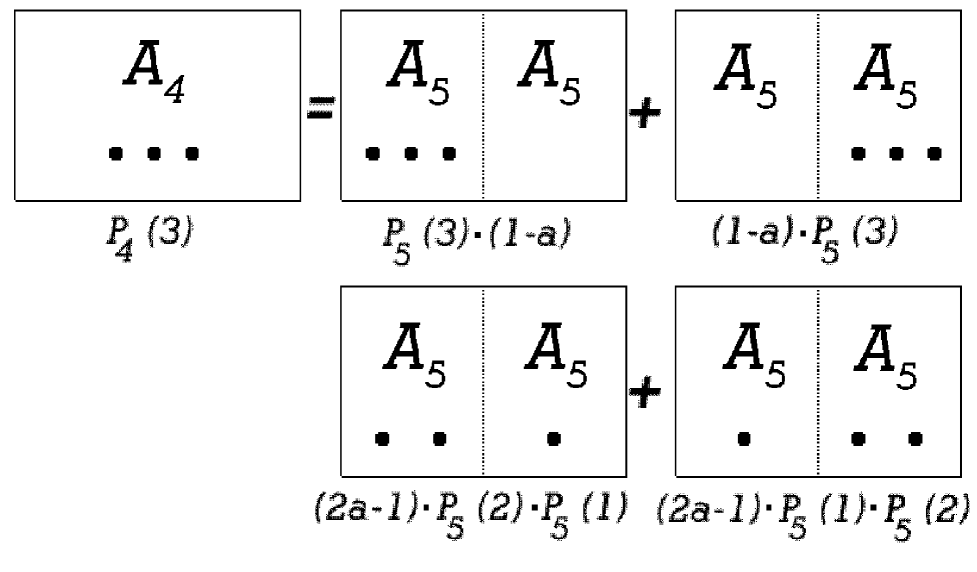
FIG. 1.: Explanation of Equation 3 . Let’s consider the case $i=4$ and $n=3$. Circles correspond to individuals of a particular species found in a patch. On the left side there are three individuals in a patch $A_{4}$, on the right side all the possible ways in which those 3 individuals can be distributed in the two patches $A_{3}$. The probability of finding three individuals in a patch $A_{4}$ is then the addition of the probability that all the individuals are on one side (prob. $1-a$) times the probability that once all the individuals are on one side there are no individuals on one side and there are three individuals on the other side (prob. $1*P_{5}(3)$) plus the probability that the species are present on both sides (prob. $2(1-a)$) times the probability that once the species are present on both sides there are two individuals on one side and 1 individual on the other one (prob. $P_{5}(2)*P_{5}(1)$). Taking $x=2(1-a)$ and $1-x=2a-1$ we find $P_{4}(3)=xP_{5}(3)+(1-x)2P_{5}(2)P_{5}(1)$. This can be generalized to obtain Equation 3. Figure taken from  [2].

where $x=2(1-a)$. This recursion relation requires an initial condition. It is supplied by defining a minimum patch $A_{m}=A_{0}/2^{m}$, such that it contains on average only one individual (see figure 2). Consequently, $P_{m}(n)=\delta_{n1}$. This also limits the maximum number of individuals that can be found in a patch $A_{i}$ to $2^{m-i}$ so $P_{i}(n)=0$ for $n>2^{m-i}$.

III The linear relation

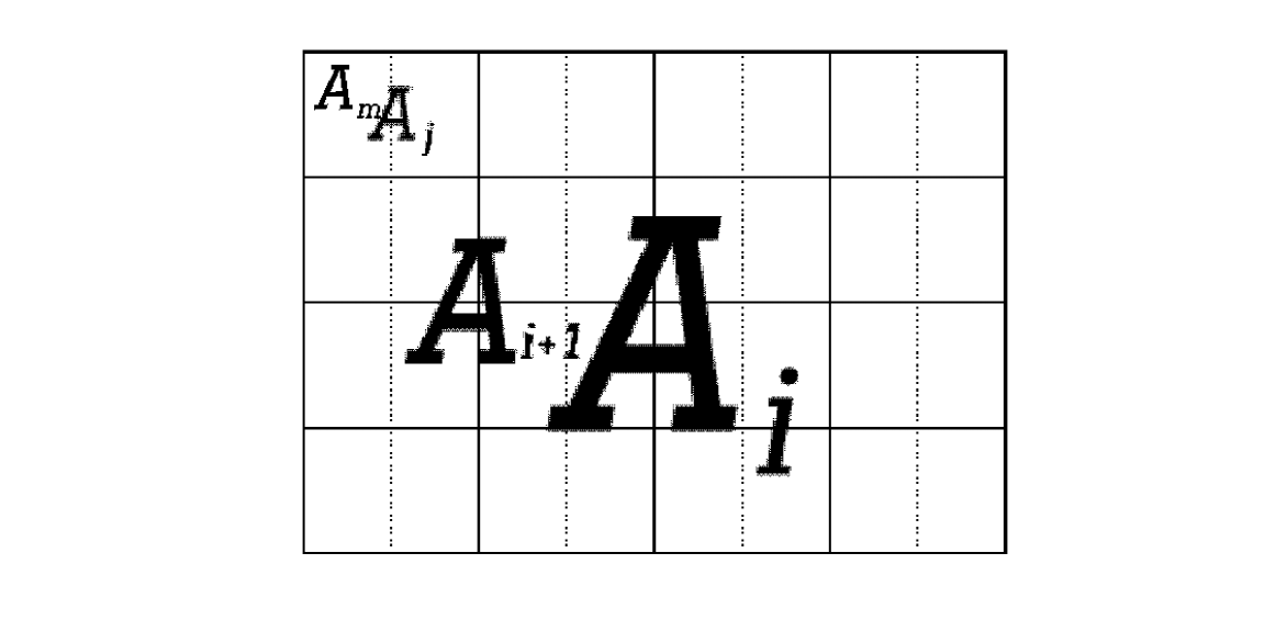
FIG. 2.: $A_{m}$ is the minimum patch. $A_{j}$ in this case comprises two minimum patches, but it can be of any size. In Equation 3 the contributions to $P_{i}(n)$ come from the two patches of size $A_{i+1}$, whereas in the case of the linear recursion relation they come from the $2^{j-1}$ patches of size $A_{j}$.

Equation 3 is nonlinear, and difficult to handle analytically. The purpose of this section is to derive an equivalent linear relation to calculate $P_{i}(n)$. This derivation sums up multiple patches at once, rather than proceeding strictly hierarchically as in the original derivation.

We consider that the contributions to $P_{i}(n)$ come from several ($2^{j-i}$) patches of area $A_{j}=A_{i}/2^{j}$ (“boxes”) instead of from 2 patches of area $A_{i+1}=A_{i}/2$ as before (see figure 2). The probability of finding $n$ individuals in $A_{i}$ is then the sum over the probabilities of finding $r$ of these “boxes” with the species present ($R_{j}^{i}(r)$), multiplied by the probability of finding $n$ individuals in these $r$ boxes ($Q_{j}^{i}(r,n)$):

$$P_{i}(n)=\sum_{r=1}^{2^{j-i}}R_{j}^{i}(r)Q_{j}^{i}(r,n)$$ (4)

Note that the index $j$ is not summed over. It is arbitrary, indicating the size of the “box”. For $j=i+1$ there are two boxes of area $A_{i}/2$ and the original result of Harte et al is recovered, whereas for $j=m-1$ we will find a linear relation. But before establishing these results we calculate explicitly $R_{j}^{i}(r)$ and $Q_{j}^{i}(r,n)$:

• $Q_{j}^{i}(r,n)$ is the probability of finding $n$ individuals in $r$ boxes of size $A_{i}/2^{j}$ in a total area $A_{i}$:

  $$Q_{j}^{i}(r,n)=$$ (5)

  $$\sum_{n_{1}\ldots n_{n}=1}^{2^{m-j}} (\prod_{l=1}^{r}P_{j}(n_{l}))\delta(n-\sum n_{k}) \hskip 5.0ptr\leq 2^{j-i}$$ (6)

  $$0 \hskip 5.0ptr>2^{j-i}$$ (7)

  This formula is the probability of finding $n_{1}$ individuals in the first box, $n_{2}$ in the second one, … etc while the Kronecker delta limits the possibilities to those that add up to the total number of individuals $n$. $2^{j-i}$ is the maximum number of boxes and $2^{m-j}$ is the maximum number of individuals in each box.

• $R_{j}^{i}(r)$ is the probability of finding $r$ boxes of size $A_{j}$ in which the species is present, in a total area $A_{i}$. This is just:

  $$R^{i}_{j}(r)=P_{m+i-j}(r)$$ (8)

  This follows because the reasoning expressed in figure 1 can be applied to find the same recursion relation for $R_{j}^{i}(r)$ as for $P_{i}(n)$:

  $$R_{j}^{i}(r)=xR_{j}^{i+1}(r)+(1-x)\sum_{k=1}^{r-1}R_{j}^{i+1}(k)R_{j}^{i+1}(r-k)$$ (9)

  The initial conditions do not change either, with $R_{j}^{j}(r)=\delta_{r1}$. The only difference with the derivation for $P_{i}(n)$ is that $r$ refers to the number of boxes (not individuals) and that the recursion has to be applied $j-i$ times instead of $m-i$ times.

We can now check that for $j=i+1$ we find the same result as before:

$$P_{i}(n) = \sum_{r}R_{1}^{i}(r)Q_{1}^{i}(r,n)$$ (10)

$$= R_{1}^{i}(1)Q_{1}^{i}(1,n)+R_{1}^{i}(2)Q_{1}^{i}(2,n)$$ (11)

Reading off from Equation (4):

$$Q_{1}^{i}(2,n) =\sum_{k=1}^{n-1}P_{i+1}(k)P_{i+1}(n-k)$$ (12)

$$Q_{1}^{i}(1,n) =P_{i+1}(n)$$ (13)

$$R_{1}^{i}(1) =x$$ (14)

$$R_{1}^{i}(2) =1-x$$ (15)

Hence we obtain:

$$P_{i}(n)=xP_{i+1}(n)+(1-x)\sum_{k=1}^{n-1}P_{i+1}(k)P_{i+1}(n-k)$$ (16)

as announced previously. To obtain a linear relation we set $j=m-1$ and obtain:

$$Q_{m-1}(r,n)=\sum_{n_{1},...n_{r}=1}^{2^{m-j}}(\prod_{l=1}^{r}P_{m-1}(n_{l}))\delta(n-\sum_{i}n_{i})$$ (17)

For $P_{m-1}(n)$ we only have the following possibilities:

$$P_{m-1}(n)=\left\{\begin{array}[]{ll}x&n=1\\ 1-x&n=2\\ 0&n\neq 1,2\par\end{array}\right.$$ (18)

We find, denoting by $q=n-r$ the number of boxes with two individuals (factors of $P_{m-1}(2)$ in the equation above):

$$g(n,r)\equiv Q_{m-1}(r,n)=\frac{r!}{(r-q)!q!}x^{r-q}(1-x)^{q}$$ (19)

The first factor is the number of possible configurations in which there are $q$ boxes with two individuals and $n-q$ with one individual. Finally we obtain:

$$P_{i}(n)=\sum_{r=1}^{2^{m-i-1}}P_{i+1}(r)g(n,r)$$ (20)

which is a linear relation involving $P_{i}(n)$ and $P_{i+1}(n)$.

IV The scaling law

Equation (13) allows us to derive the scaling law that was assumed by Banavar et al. [5]:

$$P_{i}(n)=\frac{1}{n}f(\frac{n}{N_{i}^{\phi}})$$ (21)

where $N_{i}$ $(=2^{m-i})$ is the maximum number of individuals in an area $A_{i}$ and $\phi=1-z$.

In order to achieve this, the following has to be done:

• First, find the continuum limit for $g(r,n)$. Since $g(r,n)$ is just a binomial distribution, it tends to a gaussian for large $n$:

  $$g(n,r)=\frac{r!}{(r-q)!q!}x^{r-q}(1-x)^{q}$$ (22)

  $$\approx\frac{1}{\sqrt{2\pi r}}\frac{1}{\sqrt{x(1-x)}}\exp{\left(-\frac{1}{2}\frac{(q-rx)^{2}}{rx(1-x)}\right)}$$ (23)

  $$=\frac{1}{\sqrt{\pi}\epsilon_{a,r}}\frac{1}{2{a}}\exp{\left(-\frac{(r-n/{2a})^{2}}{\epsilon_{a,r}^{2}}\right)}$$ (24)

  $$\epsilon_{a,r}=\sqrt{2(2a-1)(1-a)r/(2a)^{2}}$$ (26)

  $g(n,r)$ is the probability of finding $n$ individuals in $r$ boxes. This probability is highly peaked around $n=2ar$, since $2a$ ($=1(1-a)+1(1-a)+2(2a-1)$ ) is the average of individuals per box. The more boxes there are (bigger $r$) the sharper the peak. This means that for large $r$ the only relevant values of $n$ are those near $n=2{\bf a}r$ and the expression given above for $g(n,r)$ is valid for large $r$ (which implies large $n$).

• Second, rewrite everything in terms of a new variable $x$ and a new probability density $\overline{P}_{i}(x)$. $x$ replaces $n$ and is the fraction of the total number of species: ${n}/{N_{i}}$ (which varies from 0 to 1). $\overline{P}_{i}(n)$ is the density probability ${P_{i}(x)}/{(1/2^{m-i})}$, where $1/2^{m-i}$ is the distance between two points in the new variable $x$. In this way all $P_{i}(n)$ can be compared with each other in equal terms.

In terms of these new variables, the recursion relation can now be written as:

$$\overline{P}_{i}(x)=2\sum_{y=1/2^{m-i-1}}^{1}g(2^{m-i}x,2^{m-i-1}y)\overline{P}_{i+1}(y)$$ (27)

The continuum limit is found by taking $m$ (and consequently the number of points $N_{i+1}=2^{m-i-1}$) to an arbitrarily large value and using the continuum limit of $g(r,n)$ as defined above. The fact that the approximation for $g(r,n)$ is not a very good one for small values of $n$ or $r$ is of little importance in the limit of large $m$ :

$$\overline{P}_{i}(x) = 22^{m-i-1}\sum g(2^{m-i}x,2^{m-i-1}y)\overline{P}_{i+1}(y)\underbrace{1/2^{m-i-1}}_{\Delta y}$$ (28)

$$= \int_{0}^{1}g^{*}(x,y)\overline{P}_{i+1}(y)dy$$ (29)

where $g^{*}(x,y)=22^{m-i-1}g(2^{m-i}x,2^{m-i-1}y)$ and is equal to $\frac{1}{a}\delta(y-x/a)$ in the limit of large $m$:

$$g^{*}(x,y) = \frac{1}{\sqrt{\pi}}\frac{1}{2{a}}\frac{1}{\epsilon_{y,a}}\frac{1}{\underbrace{2^{(m-i-1)/2}}_{\delta}}\exp[\frac{(y-x/a)^{2}}{\epsilon_{y},a^{2}}\underbrace{2^{m-i-1}}_{\delta^{2}}]$$ (30)

$$= \frac{1}{\sqrt{\pi}}\frac{1}{2{a}}\frac{1}{\epsilon_{y,a}\delta}\exp{\frac{(y-x/a)^{2}}{(\epsilon_{y,a}\delta)^{2}}}$$ (31)

which is a standard representation of the Dirac delta function [6] in the $x/a$ variable for $\epsilon_{y,a}\delta\rightarrow\infty$ (or $m\rightarrow\infty$):

$$\lim_{m\rightarrow\infty}\int g^{*}(x,y)f(x)dx=f(ay)$$ (32)

$$\Rightarrow\lim_{m\rightarrow\infty}g^{*}(x,y)=\frac{1}{a}\delta(y-x/a)$$ (33)

This implies that

$$\overline{P}_{i}(x)=\frac{1}{a}\overline{P}_{i+1}(x/a)$$ (34)

which is, in terms of $n$ and $P_{i}(n)$,

$$P_{i}(n)=\frac{1}{2a}P_{i+1}(n/2a)$$ (35)

Since $a=2^{-z}$ and $\phi=1-z$, multiplying the above equation by $n$ and writing the explicit dependence of $P_{i}(n)$ on $N_{i}$ as $P_{i}(n)=P(n,N_{i})$:

$$nP(n,N_{i})=\frac{n}{2a}P(n/2a,N_{i+1})=\frac{n}{2a}P(n/2a,N_{i}/2)$$ (36)

$$\Rightarrow f(n,N_{i})\equiv nP(n,N_{i})=\frac{n}{2^{\phi}}P(n/2^{\phi},N_{i}/2)$$ (37)

which is by definition $f(n/2^{\phi},N_{i}/2)$. Since $N_{i}$ is equal to a power of two this means that $nP{i}(n)$ is a function only of $n/{N_{i}^{\phi}}$:

$$P_{i}(n)=\frac{1}{n}f(\frac{n}{N_{i}^{\phi}})$$ (38)

As can be appreciated from the results above, a constant $a$ (not dependent on $i$) is necessary to obtain the scaling law: otherwise $\phi$ would depend on $i$. In figure 3 we exhibit the scaling function for several $z$ and demonstrate the scaling law.

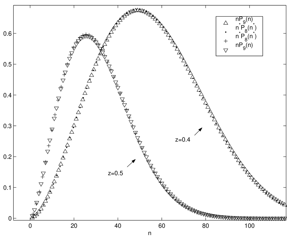
FIG. 3.: Scaling function $nP_{0}(n)=f(n/N_{i}^{\phi})$ for $m=8$ and $m=9$, and $z=0.4$ and $z=0.5$. $n^{*}\equiv n/2^{\phi}=n/2a$.

REFERENCES

• [1] M. Rosenzweig, Species Diversity in Space and Time (Cambridge Univ. Press, Cambridge, 1995).
• [2] J. Harte, A. Kinzig, and J. Green, Science 284, 334 (1999).
• [3] S. Bramwell, P. Holdsworth, and J. Pinton, Nature 396, 552 (1999).
• [4] V. Aji and N. Goldenfeld, Phys. Rev. Lett. 86, 1007 (2001).
• [5] J. Banavar, J. Green, J. Harte, and A. Maritan, Phys. Rev. Lett. 83, 4112 (1999).
• [6] C. Cohen-Tannoudji, B. Diu, and F. Laloe, Quantum Mechanics (John Wiley & Sons, New York, 1977), Vol.Β 2, p.Β 1470.