Optimizing Traffic Lights in a Cellular Automaton Model for City Traffic

Abstract

We study the impact of global traffic light control strategies in a recently proposed cellular automaton model for vehicular traffic in city networks. The model combines basic ideas of the Biham-Middleton-Levine model for city traffic and the Nagel-Schreckenberg model for highway traffic. The city network has a simple square lattice geometry. All streets and intersections are treated equally, i.e., there are no dominant streets. Starting from a simple synchronized strategy we show that the capacity of the network strongly depends on the cycle times of the traffic lights. Moreover we point out that the optimal time periods are determined by the geometric characteristics of the network, i.e., the distance between the intersections. In the case of synchronized traffic lights the derivation of the optimal cycle times in the network can be reduced to a simpler problem, the flow optimization of a single street with one traffic light operating as a bottleneck. In order to obtain an enhanced throughput in the model improved global strategies are tested, e.g., green wave and random switching strategies, which lead to surprising results.

]

I Introduction

Mobility is nowadays regarded as one of the most significant ingredients of a modern society. Unfortunately, the capacity of the existing street networks is often exceeded. In urban networks the flow is controlled by traffic lights and traffic engineers are often forced to question if the capacity of the network is exploited by the chosen control strategy. One possible method to answer such questions could be the use of vehicular traffic models in control systems as well as in the planning and design of transportation networks. For almost half a century there were strong attempts to develop a theoretical framework of traffic science. Up to now, there are two different concepts for modeling vehicular traffic (for an overview see [1, 2, 3, 4, 5, 6, 7, 8]). In the “coarse-grained” fluid-dynamical description, traffic is viewed as a compressible fluid formed by vehicles which do not appear explicitly in the theory. In contrast, in the “microscopic” models traffic is treated as a system of interacting particles where attention is explicitly focused on individual vehicles and the interactions among them. These models are therefore much better suited for the investigation of urban traffic. Most of the “microscopic” models developed in recent years are usually formulated using the language of cellular automata (CA) [9]. Due to the simple nature CA models can be used very efficiently in various applications with the help of computer simulations, e.g., large traffic network can be simulated in multiple realtime on a standard PC.

In this paper we analyze the impact of global traffic light control strategies, in particular synchronized traffic lights, traffic lights with random offset, and with a defined offset in a recently proposed CA model for city traffic (see Sec. II for further explanation). Chowdhury and Schadschneider [10, 11] combine basic ideas from the Biham-Middleton-Levine (BML) [12] model of city traffic and the Nagel-Schreckenberg (NaSch) [13] model of highway traffic. This extension of the BML model will be denoted ChSch model in the following.

The BML model [12] is a simple two-dimensional (square lattice) CA model. Each cell of the lattice represents a intersection of an east-bound and a north-bound street. The spatial extension of the streets between two intersections is completely neglected. The cells (intersections) can either be empty or occupied by a vehicle moving to the east or to the north. In order to enable movement in two different directions, east-bound vehicles are updated at every odd discrete time-step whereas north-bound vehicles are updated at every even time-step. The velocity update of the cars is realized following the rules of the asymmetric simple exclusion process (ASEP) [14]: a vehicle moves forward by one cell if the cell in front is empty, otherwise the vehicle stays at its actual position. The alternating movement of east-bound and north-bound vehicles corresponds to a traffic lights cycle of one time-step. In this simplest version of the BML model lane changes are not possible and therefore the number of vehicles on each street is conserved. However, in the last years various modifications and extensions [15, 16, 17, 18, 19, 20] have been proposed for this model (see also [8] for a review).

The NaSch model [13] is a probabilistic CA model for one-dimensional highway traffic. It is the simplest known CA model that can reproduce the basic phenomena encountered in real traffic, e.g., the occurrence of phantom jams (“jams out of the blue”). In order to obtain a description of highway traffic on a more detailed level various modifications to the NaSch model have been proposed and many CA models were suggested in recent years (see [21, 22, 23, 24, 25]). The motion in the NaSch model is implemented by a simple set of rules. The first rule reflects the tendency to accelerate until the maximum speed $v_{\text{max}}$ is reached. To avoid accidents, which are forbidden explicitly in the model, the driver has to brake if the speed exceeds the free space in front. This braking event is implemented by the second update rule. In the third update rule a stochastic element is introduced. This randomizing takes into account the different behavioral patterns of the individual drivers, especially nondeterministic acceleration as well as overreaction while slowing down. Note, that the NaSch model with $v_{\text{max}}=1$ is equivalent to the ASEP which, in its deterministic limit, is used for the movement in the BML model.

One of the main differences between the NaSch model and the BML model is the nature of jamming. In the NaSch model traffic jams appear because of the intrinsic stochasticity of the dynamics [26, 27]. The movement of vehicles in the BML model is completely deterministic and stochasticity arises only from the random initial conditions. Additionally, the NaSch model describes vehicle movement and interaction with sufficiently high detail for most applications while the vehicle dynamics on streets is completely neglected in the BML model (except for the effects of hard-core exclusion). In order to take into account the more detailed dynamics, the BML model is extended by inserting finite streets between the cells. On the streets vehicles drive in accordance to the NaSch rules. Further, to take into account interactions at the intersections, some of the prescriptions of the BML model have to be modified. At this point we want to emphasize that in the considered network all streets are equal in respect to the processes at intersection, i.e., no streets or directions are dominant. The average densities, traffic light periods etc. for all streets (intersections) are assumed to be equal in the following.

The paper is organized as follows: In the next section the definition of the model is presented. It will be shown that a simple change of the update rules is sufficient to avoid the transition to a completely blocked state that occurs at a finite density in analogy to the BML model [18, 19, 20]. Note, that this blocking is undesirable when testing different traffic light control strategies and is therefore avoided in our analyses. In Section III different global traffic light control strategies are presented and their impact on the traffic will be shown. Further it is illustrated that most of the numerical results affecting the dependence between the model parameters and the optimal solutions for the chosen control strategies can be derived by simple heuristic arguments in good agreement with the numerical results. In the summary we will discuss how the results can be used benefitably for real urban traffic situations and whether it could be useful to consider improved control systems, e.g., autonomous traffic light control.

II Definition of the Model

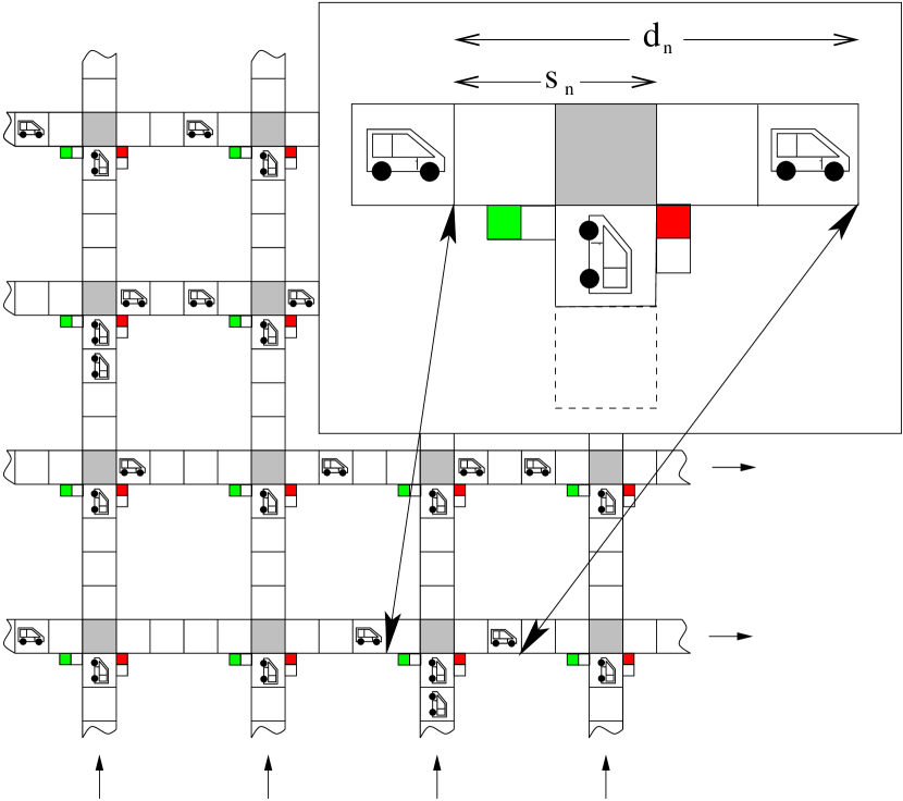
FIG. 1.: Snapshot of the underlying lattice of the model. In this case the number of intersections in the quadratic network is set to $N\times N=16$. The length of the streets between two intersections is chosen to $D-1=4$. Note that vehicles can only move from west to east on the horizontal streets or from south to north on the vertical ones. The magnification on the right side shows a segment of a west-east street. Obviously the traffic lights are synchronized and therefore all vehicles moving from south to north have to wait until they switch to “green light”.

The main aim of the city model proposed in [10] is to provide a more detailed description of city traffic than that of the original formulation of the BML model. Especially the important interplay of the different timescales set by the vehicle dynamics, distance between intersections and cycle times can be studied in the ChSch model. Therefore each bond of the network is decorated with $D-1$ cells representing single streets between each pair of successive intersections. Moreover, the traffic lights are assumed to flip periodically at regular time intervals $T$ instead of alternating every time-step ($T>1$). Each vehicle is able to move forward independently of the traffic light state, as long as it reaches a site where the distance to the traffic light ahead is smaller than the velocity. Then it can keep on moving if the light is green. Otherwise it has to stop immediately in front of it.

As one can see from Fig. 1, the network of streets builds a $N\times N$ square lattice, i.e., the network consist of $N$ north-bound and $N$ east-bound street segments. The simple square lattice geometry is determined by the fact that the length of all $2N^{2}$ street segments is equal and the streets segments are assumed to be parallel to the $x-$ and $y-$axis. In addition, all intersections are assumed to be equitable, i.e., there are no main roads in the network where the traffic lights have a higher priority. In accordance with the BML model streets parallel to the $x-$axis allow only single-lane east-bound traffic while the ones parallel to the $y-$axis manage the north-bound traffic. The separation between any two successive intersections on every street consists of $D-1$ cells so that the total number of cells on every street is $L=N\times D$. Note, that for $D=1$ the structure of the network corresponds to the BML model, i.e., there are only intersections without roads connecting them.

The traffic lights are chosen to switch simultaneously after a fixed time period $T$. Additionally all traffic lights are synchronized, i.e., they remain green for the east-bound vehicles and they are red for the north-bound vehicles and vice versa. The length of the time periods for the green lights does not depend on the direction and thus the “green light” periods are equal to the “red light” periods. At this point it is important to premention that a large part of our investigations will consider a different traffic light strategy. In the following the strategy described above will be called “synchronized strategy”. In addition we improved the traffic lights by assigning an offset parameter to every one. This modification can be used for example to shift the switch of two successive traffic lights in a way that a “green wave” can be established in the complete network. The different “traffic light strategies” used here are discussed in detail in Sec. III.

As in the original BML model periodic boundary conditions are chosen and the vehicles are not allowed to turn at the intersections. Hence, not only the total number $N_{v}$ of vehicles is conserved, but also the numbers $N_{x}$ and $N_{y}$ of east-bound and north-bound vehicles, respectively. All these numbers are completely determined by the initial conditions. In analogy to the NaSch model the speed $v$ of the vehicles can take one of the $v_{\text{max}}+1$ integer values in the range $v=0,1,...,v_{\text{max}}$. The dynamics of vehicles on the streets is given by the maximum velocity $v_{\text{max}}$ and the randomization parameter $p$ of the NaSch model which is responsible for the movement. The state of the network at time $t+1$ can be obtained from that at time $t$ by applying the following rules to all cars at the same time (parallel dynamics):

• Step 1: Acceleration:
  Step 1: $v_{n}\rightarrow\min(v_{n}+1,v_{{\rm max}})$
  

• Step 2: Braking due to other vehicles or traffic light state:

  • Case 1: The traffic light is red in front of the n-th vehicle:
    Case 1: $v_{n}\rightarrow\min(v_{n},d_{n}-1,s_{n}-1)$

  • Case 2: The traffic light is green in front of the n-th vehicle:
    Case 2: If the next two cells directly behind
    Case 2: the intersection are occupied
    Case 2: else $v_{n}\rightarrow\min(v_{n},d_{n}-1,s_{n}-1)$
    Case 2: else $v_{n}\rightarrow\min(v_{n},d_{n}-1)$
    

• Step 3: Randomization with probability $p$:
  Step 3: $v_{n}\rightarrow\max(v_{n}-1,0)$
  

• Step 4: Movement:
  Step 4: $x_{n}\rightarrow x_{n}+v_{n}$

Here $x_{n}$ denotes the position of the n-th car and $d_{n}=x_{n+1}-x_{n}$ the distance to the next car ahead (see Fig. 1). The distance to the next traffic light ahead is given by $s_{n}$. The length of a single cell is set to $7.5~{}m$ in accordance to the NaSch model. The maximal velocity of the cars is set to $v_{\text{max}}=5$ throughout this paper. Since this should correspond to a typical speed limit of $50~{}km/h$ in cities, one time-step approximately corresponds to $2~{}sec$ in real time. In the initial state of the system, $N_{v}$ vehicles are distributed among the streets. Here we only consider the case where the number of vehicles on east-bound streets $N_{x}=\frac{N_{v}}{2}$ is equal to the one on north-bound streets $N_{y}=\frac{N_{v}}{2}$. The global density then is defined by $\rho=\frac{N_{v}}{N^{2}(2D-1)}$ since in the initial state the $N^{2}$ intersections are left empty.

Note, that we have modified Case 2 of Step 2 in comparison to [11]. Due to this modification a driver will only be able to occupy a intersection if it is assured that he can leave it again. A vehicle is able to leave a intersection if at least the first cell behind it will become empty. This is possible for most cases except when the next two cells directly behind the intersection are occupied. The modification itself is done to avoid the transition to a completely blocked state (gridlock) that can occur in the original formulation of the ChSch model. Further in the original formulation [10] the traffic lights mimick effects of a yellow light phase, i.e., the intersection is blocked for both directions one second before switching. This is done to attenuate the transition to a blocked state (gridlock). Since the blocked states are completely avoided in our modification we do not consider a yellow light anymore. The reason for avoiding the gridlock situation in our considerations is that we focus on the impact of traffic light control on the network flow, so that a transition to a blocked state would prevent from exploring higher densities. Besides relatively small densities are more relevant for applications to real networks. However, taking into account that situations where cars are not able to enter an intersection are extremely rare, it is clear that this modification does not change the overall dynamics of the model. Moreover we compared the original formulation of the ChSch model and the modified one by simulations and found no differences except for the gridlock situations which appear in the original formulation due to the stronger interactions between intersections and roads.

III Strategies

As mentioned before our main interest is the investigation of global traffic light strategies. We want to find methods to improve the overall traffic conditions in the considered model. At this point it has to be taken into account that all streets are treated as equivalent in the considered network, i.e., there are no dominant streets. This makes the optimization much more difficult and implies that the green and red phases for each direction should have the same length. For a main road intersection with several minor roads the total flow usually can be improved easily by optimizing the flow on the main road.

We first study the dependence between traffic light periods and aggregated dynamical quantities like flow or mean velocity. It is shown that investigating the simpler problem of a single road with one traffic light (i.e., $N=1$) operating as a defect is sufficient to give appropriate results concerning the overall network behavior. The results can be used as a guideline to adjust the optimal traffic light periods in respect to the model and network parameters. Further we show that a two dimensional green wave strategy can be established in the whole network giving much improvement in comparison to the synchronized traffic light switching. Finally we demonstrate that switching successive traffic lights with a random shift can be very useful to create a more flexible strategy which does not depend much on the model and network parameters. Throughout the paper we will always assume that the duration of green light is equal to the duration of the red light phase.

A Synchronized Traffic Lights

FIG. 2.: The mean flow $J$ of the smallest network segment (one single intersection, $N=1$) is plotted for different global densities as a function of the cycle length $T$. For the top part of the figure we use a randomization parameter of $p=0.1$ while in the bottom plot higher fluctuations $p=0.5$ are considered. In both cases the free-flow regime (density $\rho=0.05$) shows a similar shape. The high density regime reflects a stronger dependence on the randomization parameter, but also for the higher $p$ strong variations of the mean flow can be found. The length of the street is $L=100$ and the flow is aggregated over $100.000$ time-steps.

The starting point of our investigations is the smallest possible network topology of the ChSch model. Obviously this is a system consisting of only one east-bound and one north-bound street, i.e., $N=1$, linked by a single intersection. As a further simplification we focus on only one of the two directions of this “mini” network, i.e., a single street with periodic boundary conditions and one signalized cell in the middle. It is obvious that in the case of one single traffic light the term “synchronized” is a little bit confusing, but the relevance of this special case to large networks with synchronized traffic lights will be discussed later.

Fig. 2 shows the typical dependence between the time periods of the traffic lights and the mean flow in the system. For low densities one finds a strongly oscillating curve with maxima and minima at regular distances. In the case of a small fluctuation parameter $p$ similar oscillations can be even found at very high densities. For an understanding of the underlying dynamics leading to such strong variations in the mean flow we take a look into the microscopic structure. This will allow us to formulate a simple phenomenological approach which shows a very good agreement with numerical results. Note that we restrict our investigations to low densities because for free-flow densities vehicles are not constricted by jamming due to the model dynamics, but rather by “red” traffic lights. Hence the free-flow density range shows the largest potential for flow optimization. Later on we will point out the origin of the oscillating flow even at very high densities which is completely different to the free-flow case.

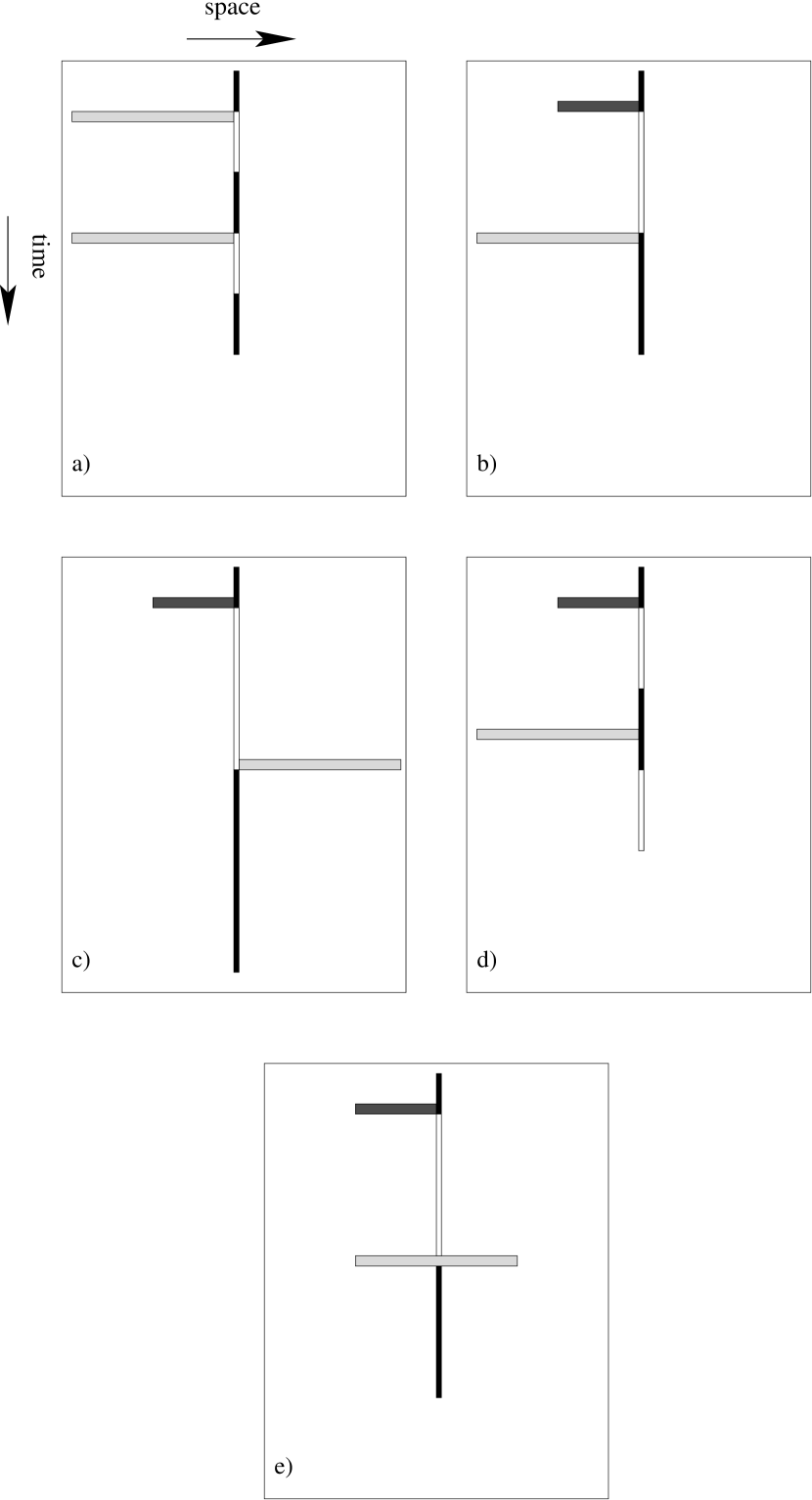
FIG. 3.: Schematic representation of the vehicle movement on the east bound street for different cycle times. Standing cars are represented by dark grey rectangles ($x$-axis) while moving vehicle clusters are bright grey rectangles. The traffic light is placed in the middle of every figure (time runs along the $y$-axis). Its state is indicated by the colour of the vertical rectangle. Green light corresponds to the white colored area of the traffic light while red light is painted in dark. At this point one has to take into account that the considered street has periodic boundary conditions and therefore vehicles leaving the right end of every scenario (a)–(e) will return after a certain time on the left side.

To give an impression of the influence of the cycle times on the vehicle movement a schematic representation of the observed street is depicted in Fig. 3. This picture covers typical dynamical patterns occurring in the system due to vehicles which are restricted in their movement by the “red light”. Based on these scenarios a simple phenomenological approach is presented in the following which is able to explain the dependence between vehicle movement and model parameters. We assume that during one traffic light cycle free-flowing vehicles form a stable cluster with a width which is approximately constant. Further we assume that a phase separation between free-flowing and jammed vehicles takes place at high densities. The legitimation for these assumptions is given by the fact that the vehicle movement is triggered by the traffic light, i.e., vehicles are gathered in front of the them and hence fluctuations can not spread out. In addition, the cycle length is of the order of the street length or more precisely, the travel time from one intersection to the next. It makes no sense to consider cycle times that are much larger than the travel time which is proportional to the length of the street segment. Note that the limit $T\to\infty$ corresponds to the case in which one direction of the network is free to move all the time while on the other direction it comes to a complete stop. The resulting flow then is exactly half of the flow found in the underlying NaSch model.

In the following we focus on five scenarios (a)–(e). The cases (a), (b) and (c) describe the derivation of the maxima/minima of the $(v,T)-$curve, (d) gives a calculation of the mean velocity between maxima and minima, and (e) finally a calculation of the mean velocity between the minima and maxima. We now discuss these scenarios in more detail. Note that they are quasi-deterministic and can be slightly modified in the presence of fluctuations.

(a) The time a free flowing vehicle requires to move from one intersection to the succeeding one (one full turn on the periodic street for $N=1$) is equal to

$$T_{\text{free}}=\frac{D}{v_{\text{free}}},$$ (1)

where $v_{\text{free}}=v_{\text{max}}-p$ is the free-flow velocity of the underlying NaSch model. In Fig. 3a a situation is displayed where vehicles organize in a cluster (light grey rectangle) which can move ahead all the time. This is only possible if the time for one complete traffic light cycle, i.e., including green and red phase, is equal to the cycle time of a vehicle $T_{\text{free}}=T_{\text{green}}+T_{\text{red}}=2T$. Obviously this case corresponds to a maximum in flow whereby the traffic light period is given by $T=T_{\text{free}}/2$. Additionally there are further maxima when $T_{\text{free}}=n(T_{\text{green}}+T_{\text{red}})$ with ($n=0,1,2,...$). Thus the traffic light period corresponding to a maximal system flow is given by:

$$T_{\text{max}}=\frac{T_{\text{free}}}{2n}.$$ (2)

With similar arguments the occurrence of minima can be explained. These minima correspond to situations where the traffic lights switch exactly to red when a vehicle cluster reaches a intersection. It is clear that the assumptions above are only valid for very short cycle times $(2T\leq T_{\text{free}})$. In the following we will concentrate on more realistic “larger” periods, i.e. $2T\geq T_{\text{free}}$.

(b) In Fig. 3b a situation is shown where vehicles are gathered in front of a red light. After the traffic light switches to green the vehicles start moving. Then it switches back to red exactly at the time when the first car of the moving vehicle cluster reaches the intersection again. Now the complete vehicle cluster comes to rest and has to wait until the traffic light switches again to green to continue the movement. Obviously this case corresponds to a minimum in the flow. The corresponding cycle time is given by the following assumptions. For this scenario it is sufficient to focus on the first car of the cluster. At the beginning the first vehicle has to accelerate to its maximum velocity. This acceleration process will take on average $T_{\text{acc}}=\frac{v_{\text{max}}}{1-p}$ time-steps. After that the vehicle has to trespass the rest of the street until it reaches the intersection again. The mean velocity on that part of the road is given by $v_{\text{free}}$. The length of this road segment is given by the length of the street minus the distance that the vehicle has covered during its acceleration phase. Therefore, the time $T_{\text{first}}=\frac{D-T_{\text{acc}}(v_{\text{max}}+1)/2}{v_{\text{free}}}$ elapses until the intersection is reached. In summary, if the chosen cycle time is equal to

$$T_{\text{min}}=T_{\text{acc}}+T_{\text{first}}+nT_{\text{free}},$$ (3)

the system flow is minimal. The last term $nT_{\text{free}}$ (with $n=0,1,2...$) takes into account traffic light periods that are larger than the required time to move from one intersection to the succeeding one or to make one turn on a periodic system. That way the vehicle cluster is able to perform $n$ “turnarounds” before it has to stop immediately in front of the “red light”. These minima at regular distances of $T_{\text{free}}$ time-steps can be easily identified in Figs. 2, 4.

(c) In accordance with the occurring minima one can also find maxima at regular distances (see Figs. 2, 4). These maxima correspond to situations where the length of the green time intervals is sufficiently large so that the last vehicle of a moving cluster is able to pass the intersection before the traffic light switches to red. To derive the cycle times corresponding to this situation one has to focus on the last car. Before the traffic light switches to green there are $N_{\text{wait}}$ vehicles standing in front of it (dark grey rectangle) (see Fig. 3c). After the switch to green the last vehicle of the cluster has to wait on average $T_{\text{wait}}=\frac{N_{\text{wait}}-1}{J_{\text{out}}}$ time-steps before the vehicle in front started to move ($J_{\text{out}}$ is equal to the flow out of a jam). Then further $T_{\text{acc}}$ (see case (b)) time-steps are needed for the vehicle to accelerate to its maximum velocity. From then on the vehicle has to reach the first cell (behind the intersection) of the succeeding street within the remaining “green light” interval. The required time to cover this part of the road is given by $T_{\text{last}}=\frac{D+N_{\text{wait}}-T_{\text{acc}}(v_{\text{max}}+1)/2}{v_{\text{free}}}$. Note, that in comparison to case (b) the last vehicle has to cover a slightly larger distance than the first one due to its shifted starting position of about $N_{\text{wait}}$ cells. Therefore, the system is in a state with of maximum flow for the following cycle times:

$$T_{\text{max}}=T_{\text{wait}}+T_{\text{acc}}+T_{\text{last}}+nT_{\text{free}}.$$ (4)

As in (b), the last term $nT_{\text{free}}$ takes into account large cycles where the vehicle cluster is able to make $n$ full turns before the pictured situation occurs.

(d) We used the previous cases (a)–(c) as a basis for simple heuristic arguments to derive the cycle times corresponding to maximal and minimal mean flow states in the system. In the remaining cases we will show that even the complete dependence of the mean velocity on the cycle time can be obtained from simple phenomenological assumptions. For this purpose we focus on a situation where the vehicle cluster is able to cross the intersection within the “green light”, i.e., the traffic light does not switch when the vehicle cluster occupies the intersection. After the vehicle cluster has passed the intersection at most $n$ times the vehicles will come to a rest in front of a “red light”. The remaining waiting time depends now on the chosen cycle time. If the traffic light switches to red immediately before the vehicles reach the intersection the situation corresponds to minimal flow (see (b)), i.e., the vehicles must wait for the complete cycle time $T$. Contrary, if the traffic light switches directly after the cluster has trespassed the intersection the situation corresponds to the case of maximal flow (see (c)), i.e., the vehicle cluster can perform a complete turn within a “red light” phase and therefore the remaining waiting time gets minimal. The more general case is given by a situation between maximal and minimal flow, i.e., the vehicle cluster is able to pass the intersection and then after a certain time the traffic light switches to “red light”. To obtain the mean velocity of the vehicles within a complete cycle $T_{\text{cycle}}=2T$ neither one has to take into account the waiting times of vehicles in the starting phase nor the acceleration process of the vehicles until the maximum velocity is reached. In fact only the driven distance which is equal to $n$ turnarounds for every vehicle must be considered in order to obtain the mean velocity. Note, that each vehicle starts its movement out of a certain position in a waiting queue in front of the traffic light and will occupy exactly the same position when it comes to a rest again. The mean velocity is given by

$$\overline{v}_{\text{max--min}}(T,n)=\frac{nD}{2T}.$$ (5)

With Eqn. (5) it is possible to plot the mean velocity of the system against the traffic light periods only between each $n$-th maximum and $n$-th minimum of the curve. The shape of the curve between the $n$-th minimum and the $(n+1)$-th maximum will be discussed in (e). One should keep in mind that the scenarios (b)–(e) assume $T\geq T_{\text{free}}$.

(e) In Fig. 3e a situation is pictured where the traffic light switches to “red light” within the time interval at which the vehicle “cluster” crosses the intersection. As a consequence the fraction of vehicles in front of the traffic light will come to a stop while the rest of the vehicles behind it is able to move on until they reach the traffic light again (periodic boundary conditions). The fact that only a fraction of vehicles is able to complete $n$ cycles whereas other can complete $n+1$ cycles before they are forced to stop leads to a simple linear dependence between the mean velocity and the cycle time in this area.

FIG. 4.: Top: The mean velocity $v_{\text{mean}}$ for a minimal network $N=1$ is plotted against the cycle time $T$. The street has a length of $L=100$ cells and the density is set to $\rho=0.05$ (free-flow case). One can clearly see that the phenomenological approximation agrees very well with the simulation data. Bottom: In order to show, how the small network segment with $N=1$ (considered in the heuristic approach) compares to the complete ChSch city network model we plotted the mean flow against the traffic light period $T$. This is done once for the “mini network” consisting of one single intersection with a street length of $L=100$ cells and for a relatively large network consisting of $N\times N=100$ intersections with $2N^{2}$ street segments each of $D=100$ cells in length. We consider two different densities, one of them corresponding to the free-flow density $\rho=0.05$ and the other to a high density state $\rho=0.7$. Obviously, the deviations in the curves between the large network and the “mini network” are negligible in both density regimes. The randomization parameter is $p=0.1$ and the maximum velocity is $v_{\text{max}}=5$ in both diagrams.

In the left part of Fig. 4 we show how the mean velocity of the north bound street of the considered “mini network” depends on the cycle time and compare these results with the phenomenological predictions made in (a)–(e). As one can see the theoretical curve shows an excellent agreement with the simulation data. Not only the positions of the maxima and minima are predicted by theory but also the shape of the curve between the extrema shows a very good agreement with the numerical results. At this point we want to emphasize that we checked the mean velocity on the east bound street as well and found exactly the same results. This is not further surprising if one takes into consideration that the duration of the traffic light cycles of both directions are the same, i.e., the time of “red light” is equal to the “green light” and when the north-bound direction switches to green then the east-bound direction switches to red and vice versa. Therefore the two different directions can be considered as almost decoupled and independent. Furthermore the right part of Fig. 4 shows that the results obtained from the observed “mini network” are completely transferable to large networks. Thus we stress that the assumptions made in (a)–(e) can be used to adjust the optimal cycle times in large networks, i.e., in the ChSch model with synchronized traffic lights. The excellent agreement between the small and the large network situation can be ascribed to the synchronized strategy. In fact, there is no difference for a vehicle approaching an intersection which is a part of a large network or approaching the only existing intersection due to the periodic boundary conditions. The state of the traffic lights will be the same in both cases because of the synchronized strategy. Moreover it is very interesting that although the vehicle movement is stochastic (NaSch model) and the mean density on the streets in the network fluctuates, there is no local concentration of vehicles in the network leading to remarkable deviations in the flow in comparison to the idealized “mini network” where the density on the streets is fixed. Note, that this is in contrast to the original formulation of the ChSch model where a blockage of intersections is allowed. Therefore fluctuations can lead to a complete breakdown of flow at high densities where standing vehicles are gathered in one part of the network. It seems that the signalized intersections of the model interact with the density fluctuations in a way that the vehicles are equally distributed in the network. The extreme fluctuations in the distribution do not play an important role in progress of time because the blockage of an intersection due to such fluctuations is excluded here (see sec. II) and so the density on the roads fluctuates around a mean value.

The results obtained by the phenomenological approach confirm that the dynamics in the network is driven by the traffic lights and mainly determined by the distance between them and the density of cars. It seems that the influence of the model chosen for the vehicle movement plays a secondary role. We only assume the mean velocity of free flowing vehicles and the outflow out of a jam as parameters for the movement from the underlying NaSch model. To verify this, we investigate a comparable network scenario where the vehicle movement is realized by the VDR model [21]. A major difference to the NaSch model is the occurrence of large phase separated jams and metastable states in the absence of intersections. However, we found qualitatively the same results for both models assuming the outflow of a jam and the mean velocity as parameters. One reason is that the metastable states of the VDR model are destroyed by disturbances caused by the traffic lights.

So far we have only observed the free-flow case of the ChSch model in our scenarios. But also for high densities one can find a strong dependence of the mean flow in the system on the chosen cycle times (see Fig. 2). Obviously for high densities this dependence is not caused by free flowing vehicle clusters passing or not an intersection, but rather due to the movement of large jams gathered in front of the traffic lights. These jams move oppositely to the driving direction. For densities slightly above the free-flow density (see $\rho=0.2$ in Fig. 2) there are no characteristic maxima or minima in the mean flow. Here the remaining jams in the system are small compared to the cycle times, i.e., the time a jam will block an intersection is negligible small. Furthermore, for decreasing traffic light cycles, large jams are divided into smaller ones by the short cycle times. Thus, the mean flow increases slightly with higher cycle times in this density area because the number of standing cars decreases. At intermediate densities (see $\rho=0.5$ in Fig. 2) one can find a similar behavior. As for $\rho=0.2$ the number of jams decreases with increasing cycle times and the flow grows slightly until it breaks down at a certain value. This breakdown can be explained as follows: At high cycle times only one jam remains between two intersections because the “red light phase” is large enough so that all vehicles are gathered in front of the traffic lights. The breakdown finally occurs when the “red light phase” is even larger than the time needed to conglomerate all vehicles in front of it. As a consequence, the vehicles have to wait considerably longer than they are able to move when further increasing the cycle time. Note, that the motion at “green light” is hindered because of the fact that for the considered densities the jam is relatively large. Therefore a intersection is blocked when it is reached by the backward moving jam for a long part of the “green light phase”. It is interesting that for high densities (see $\rho=0.7$ in Fig. 2) a strong dependence between the cycle time and the mean flow can be found with characteristic maxima and minima similar to the free-flow case. This is caused by the fact that at high densities the dynamics of the system is completely determined by the movement of a jam. For example, if the length of one cycle (red light and green light) is chosen in such a manner that it is equal to the time the downstream front of a jam needs to move from one intersection to the next one, the large jam will block the intersection when it is red anyway. This corresponds to a maximum in the global network flow. The fraction of time when the “red-light” has no influence on the mean flow because it is blocked by a jam determines the shape of the curve between the extrema similar to the free-flow scenarios. For a more detailed discussion, see [28]. At this point we want to emphasize that high densities are more difficult to investigate because the jamming in the NaSch model is strongly determined by the fluctuation parameter. For higher $p$ spontaneous jams can occur even in the outflow region of a jam and therefore jams are not compact anymore. At high densities one can see a relatively strong influence of $p$ while in the free-flow case the value of the randomization parameter $p$ does not play an important role.

B Green Wave Strategy

FIG. 5.: In order to compare the gain of a network operating with a “green wave” strategy to a system with a synchronized strategy we plotted the flow against the cycle time for both systems. The top diagram shows the free-flow case of the system. As one can see, the green wave strategy (time delay $T_{\text{delay}}=10$) shows reasonable improvements over the network with synchronized traffic lights $T_{\text{delay}}=0$. Moreover for comparing the green wave strategy with a network consisting of only one intersection, but an equal total street length, one finds a remarkable agreement. The bottom diagram shows the influence of the green wave strategy in the high density state. It its obvious that by definition no green wave can be established in the system because the density is too high, so that no jam free states can be obtained. Nonetheless, the performance of the network with synchronized traffic lights is exceeded by the “green wave” strategy. The randomization parameter is $p=0.1$ and the maximum velocity is $v_{\text{max}}=5$.

In the previous section we discussed the dependence between traffic light periods and throughput in the ChSch model for synchronized traffic lights. It was shown that the whole problem can be reduced to an analysis of a single segment (i.e., $N=1$) of the network. This indicates that synchronizing the traffic lights is an ineffective strategy which is not capable to bring an additional gain out of the network topology. Further it was shown that particularly at free-flow densities there are strong oscillations in the throughput of the network depending on the chosen traffic light periods. Another disadvantage is, as one can see in Fig. 2, that the first maxima are located at unrealistic short cycle times for the chosen street length.

In the following we will introduce a simple “green wave” strategy in order to improve the overall network throughput. Therefore the ChSch model is enhanced by traffic lights which are not enforced to switch simultaneously. The intersections are denoted with indices $i,j$ where $i=0,1,..,N-1$ represents the rows and $j=0,1,..,N-1$ the columns of the quadratic network. In addition, an individual offset parameter $\Delta T_{i,j}$ is introduced and assigned to every intersection. This offset parameter is used to implement a certain time delay $T_{\text{delay}}$ between the traffic light phases of two successive intersections. The offset parameter itself can take the values $\Delta T_{i,j}=0,...,2T$. Note, that a larger $\Delta T_{i,j}$ has no effect because $2T$ corresponds to one complete cycle of a traffic light. The main intention when establishing a “green wave” on an intersected street is to keep a cluster of vehicles in motion. It is obvious that the optimal strategy is to adjust the time delay between two successive intersections such that the first vehicle of a moving cluster trespassing an intersection will arrive at the next traffic light exactly at the time when it switches to “green”. This delay is just the time a free flowing vehicle needs to move from one intersection to the succeeding one, i.e., $T_{\text{free}}=\frac{D}{v_{\text{free}}}$. Thus this is the optimal time delay $T_{\text{delay}}$ between two intersections. Since we are interested in constituting the “green wave” in the whole network, two directions must be taken into account. We choose the intersection at the bottom left corner of the network as the starting point with no time delay $\Delta T_{0,0}=0$. Then the offset in the first row will be chosen as described, i.e., the time delay between two successive intersections is in the optimal case equal to $T_{\text{free}}$. After the first row is initialized every intersection in this row will be seen as a new starting point to initialize the corresponding columns. In summary, the offset parameter of the intersections is given by

$$\Delta T_{i,j}=((i+j)T_{\text{delay}})\ \text{mod}(2T),\\ (i,j=0,1,..,N-1),$$ (6)

with the optimal offset parameter given by $T_{\text{delay}}=T_{\text{free}}$, i.e.,

$$\Delta T_{i,j}=\left((i+j)\frac{D}{v_{\text{free}}}\right)\text{mod}(2T),\\ (i,j=0,1,..,N-1).$$ (7)

Using this method a two-dimensional “green wave” strategy can be established in the ChSch model.

To quantify the improvement obtained by the “green wave” strategy the overall network flow is plotted against the cycle time (see Fig. 5) and compared with the synchronized strategy. The left diagram corresponds to the free-flow case of the system. The density is chosen to $\rho=0.05$ to ensure that moving vehicles are able to drive from one intersection to the next one without being constricted by standing cars. Obviously, the green wave strategy with a properly chosen offset parameter, i.e., for the considered street length equal to $T_{\text{free}}=T_{\text{delay}}=10$, shows reasonable improvements over the strategy with synchronized traffic lights ($T_{\text{delay}}=0,N=4$). The whole spectrum of plotted cycle times $T$ for the “green wave” strategy exceeds the performance of the network with synchronized traffic lights or at least keeps the performance. Moreover, comparing the green wave strategy to a network consisting of only one intersection, but with the same total street length, one finds a remarkable agreement of the curves. Note, that every street in the considered network with $N=4$ is intersected four times. We want to stress here that for free-flow densities in the ChSch model the “green wave” strategy is capable to pipe all vehicles through the streets, i.e., for the vehicles on the streets it seems as if there is only one intersection in the system left due to the fact that the remaining ones are always green when approached by the vehicle cluster. Further we want to point out that similar to the case with a synchronized strategy the traffic lights interact with the vehicles in such a way that a “green wave” is established in the network independent of the initial vehicle distribution or the density fluctuations caused by the internal stochasticity of the model. Recapitulating, one of the most important benefits of the green wave strategy is the fact that a street with total length $L$ consisting of $N$ street segments, each with a length $D$, behaves like a street intersected only once (see Fig. 5). Therefore the optimal cycle time of a traffic light corresponding to the maximal flow is shifted towards realistic values (see Sec. III Aa) even for small street segment lengths $D$. One obtains the following equation for the cycle time corresponding to maximal flow (see Eqn. 2):

$$T_{\text{max}}=\frac{L}{2v_{\text{free}}}=\frac{ND}{2v_{\text{free}}}.$$ (8)

As one can see in the right part of Fig. 5 even for high densities the “green wave” strategy shows an incisive impact to the network flow. Although by definition no “green wave” can be established at high densities (for the chosen density of $\rho=0.7$ no jam free state can exist), an offset in the switching between successive traffic lights can lead anyhow to an improved flow. The origin of this improvement is completely different in comparison to the free-flow case. For low densities the dynamics is driven by vehicles organized in clusters which can move through the streets undisturbed due to the optimal strategy whereas the dynamics for high densities is governed by the motion of large jams. Large jams move oppositely to the driving direction of the vehicles from one intersection to the one before. Due to their spatial extension a intersection is blocked for a certain time when trespassed by a jam. Thus the optimal system state would be reached if a jam moves backward from one intersection to the one before and blocks it while the traffic light is red anyway so that afterwards moving vehicles (outflow of the jam) can take advantage of the green phase as much as possible. In fact, the portion of time that a intersection is blocked or free determines the system flow. Note, that the time delay at high densities has to be negative since jams move opposite to the driving direction. For a time delay in the order of the optimal time delay of the free-flow case (see Fig. 5 (right) for $T_{\text{delay}}=-10$) the curves corresponding to the “green wave” strategy and the synchronized traffic lights do not differ much because this $T_{\text{delay}}$ is determined by the free vehicle movement. Considering instead the velocity of a jam which is approximately about $v_{\text{jam}}=\frac{1}{1-p}$ (see [29]) and assuming that the optimal time delay is the travel time $T_{\text{jam}}=\frac{D}{v_{\text{jam}}}$ for the backward motion of a jam between two intersections, the difference to the synchronized case gets transparent (see Fig. 5 (right) for $T_{\text{delay}}=-55$). The “green wave” strategy allows now a reasonable improvement over the synchronized strategy. Similar to the free-flow density case, the performance of the network with synchronized strategy is exceeded by the “green wave” strategy for almost all cycle times. Moreover, comparing the “green wave” strategy with an optimal time delay to an idealized “mini network” consisting of only one intersection, but with an equal total street length one finds an reasonable agreement between the curves as well. This indicates that for high densities jams can be guided perfectly through the streets by a “green wave” strategy. However, one has to recognize that strong oscillations at high densities depend on the statistics of the underlying NaSch model so that the expected gain at these high densities will decrease with increasing $p$.

C Random Offset Strategy

FIG. 6.: The random offset strategy is compared to the original ChSch model with synchronized traffic lights. The mean flow is plotted versus the traffic light periods for the two different strategies. The network consists of $N\times N=100$ intersections with $2N^{2}$ street segments each of length $D=100$ cells. Top: In the left part of the Fig. we chose a low density (free-flow regime, $\rho=0.05$). It can be seen clearly that the oscillations found in the synchronized network are suppressed by the random offset strategy. Furthermore in the free flow density regime the random offset strategy shows some advantages over the synchronized strategy, but only for low cycle times. Bottom: The oscillations for high densities ($\rho=0.70$) are suppressed in a similar manner as for the low density case. In addition, the random offset strategy seems to outperform the synchronized strategy in the whole plotted area. The randomization parameter is $p=0.1$ and the maximum velocity is $v_{\text{max}}=5$.

In this section we want to point out that switching successive traffic lights with a random shift instead of a fixed time delay can lead to a more flexible strategy, e.g., without oscillations. Moreover it will be shown that in contrast to a system with synchronized traffic lights a random shift between the intersections can lead to a remarkable higher global system flow. As in the previous section the traffic lights are not enforced to switch simultaneously anymore. For this purpose an individual offset parameter $\Delta T_{i,j}$ is introduced and assigned to every intersection (see previous section for a detailed explanation). The offset parameter itself can take values between $\Delta T_{i,j}=0,...,2T$ which are chosen in the following from an equally distributed random distribution.

To give an insight into the effects induced by random offsets we depicted the throughput in the network in dependence of the cycle times in Fig. 6. The random offset strategy is compared to the ChSch model with synchronized strategy. Obviously the strong oscillations found in the curves corresponding to the synchronized strategy are destroyed by the randomness in the switching. Thus the random offset strategy leads to a smoothed curve which is very useful adjusting the optimal cycle times in a network. One is no longer forced to pay strong attention to the cycle times like in systems with synchronized or “green wave” strategies.

The left part of the Fig. 6 shows a system with free-flow density $\rho=0.05$. The random offset strategy outperforms the synchronized strategy only for relatively low cycle times because unfavorable states (states with minimal global flow) are avoided by the randomness. For higher cycle times the global flow in a system with random offset strategy falls clearly below the global flow in a system with synchronized strategy. In the case of a system with synchronized traffic lights the curve converges in the limit $T\to\infty$ to the half of the flow found in the NaSch model. This corresponds to the case in which vehicles in the network are free to move in one direction all the time while in the other direction it comes to a complete stop. In contrast, the flow in the random offset strategy converges to zero since the switching is not synchronous and therefore the traffic lights along one direction are green or red at random so that all vehicles are gathered in front of the red lights. Additionally, one has to consider that although the random offset strategy is very effective for low cycle times one can obtain higher flows with the “green wave” strategy.

At high densities ($\rho=0.70$ in Fig. 6), the oscillations are suppressed in a similar manner as for the low density case. Hence, as for low densities, this strategy gives an improved flexibility when adjusting optimal cycle times in the network. In addition, the random offset strategy outperforms the synchronized strategy not only for low cycle times, but also in the whole range plotted in Fig. 6 except for some peaks. One obvious explanation for the profit out of the randomly switching traffic lights is that parts of the network are completely jammed while in other parts of the network the cars can move nearly undisturbed. However, the flow obtained by the “green wave” strategy is still remarkably higher than the flow obtained by the random offset strategy. Furthermore one has to consider that the strong oscillations at high densities depend on the statistics of the underlying NaSch model so that the expected gain at this high densities will decrease with increasing randomization parameter $p$. Thus we want to point out that among the analyzed global strategies the “green wave” strategy leads to the highest global flow in the network for free-flow densities as well as for high density states while the “random offset” strategy provides the greatest flexibility hence the oszillations are suppressed.

IV Summary and Discussion

We have analyzed the ChSch model which combines basic ideas from the Biham-Middleton-Levine (BML) model of city traffic and the Nagel Schreckenberg (NaSch) model of highway traffic. In our investigation we focused on global traffic light control strategies and tried to find optimal model parameters in order to maximize the network flow. For this purpose we started with the original formulation of the ChSch model where the traffic lights are switched synchronously. It is shown that the global throughput of the network strongly depends on the cycle times, i.e, one finds strong oscillations in the global flow in dependence of the cycle times both for low as well as for high densities. A simple phenomenological approach has been suggested for the free-flow regime in order to determine the characteristics in regard to the model parameters and to obtain a deeper insight into the dynamics in the network. The phenomenological results show a very good agreement to numerical data and indicate that the choice of the underlying model for vehicle movement between intersections does not play an important role. Thus we want to stress here that the global throughput in the ChSch model is mainly determined by the travel times between intersections which depends on the length of the street segments and the density and maximal velocity of the cars.

In order to allow a more flexible traffic light control the ChSch model was enhanced by an additional model parameter. This new parameter is assigned to every intersection representing a time offset, so that the traffic lights are not enforced to switch simultaneously anymore. A two dimensional “green wave” is implemented with the help of the new parameter. The “green wave” gives much improvement to the flow in comparison to the synchronized strategy at low densities and has even an incisive impact on the throughput at high densities. Moreover it is shown that the influence of intersections along a street is completely avoided by the “green wave” strategy because the results can be compared with results obtained from a system containing only one single intersection instead of many others. Although the “green wave” strategy is capable to give a strong improvement, the dependence between flow and the cycle time found in the original ChSch model remains. Thus to avoid this strong oscillations we further analyzed a network where traffic lights are switched at random. It is shown that the strong oscillations found for a synchronized strategy and for the “green wave” strategy are completely suppressed by randomness. Thus the random offset strategy can be very useful if a control strategy is required which is not very sensitive to the adjustment of the cycle times. Moreover, the random offset strategy outperforms the standard ChSch model with synchronized traffic lights at low densities for small cycle times and at high densities for all cycle times. An explanation for the profit at high densities is the fact that some parts of the network are completely jammed while in other parts of the network the cars can move nearly undisturbed. This additional gain due to the inhomogeneous allocation of vehicles indicates that an autonomous traffic light control based on local decisions could be more effective than the analyzed global shemes. In [30] Faieta and Huberman investigated an autonomous traffic light strategy which shows a very good performance. Results of simulations with the ChSch model about the impact of traffic lights which are autonomously adapted to the traffic conditions by suitable parameters will be presented in [31].

To conclude, the results presented here are of practical relevance for various applications of city traffic. Due to its simplicity cellular automata models have become quite popular for large scale computer simulations whereby especially city traffic with its complex network topology is one of the favorable applications. In particular the knowledge of the impact of topological factors in regard to certain traffic control strategies can be very benefitable when studying various kinds of city networks, even those with a more sophisticated topology than those implemented in the ChSch model.

Acknowledgement:
We thank Torsten Huisinga, Wolfgang Knospe, and Andreas Pottmeier for useful discussions.

REFERENCES

- [1] D.E. Wolf, M. Schreckenberg, and A. Bachem (eds.), Traffic and Granular Flow (World Scientific, 1996).
- [2] M. Schreckenberg and D.E. Wolf (eds.), Traffic and Granular Flow ‘97 (Springer, 1998).
- [3] D. Helbing, H.J. Herrmann, M. Schreckenberg, and D.E. Wolf (eds.), Traffic and Granular Flow ‘99 (Springer, 2000).
- [4] I. Prigogine and R. Herman, Kinetic Theory of Vehicular Traffic (Elsevier, Amsterdam, 1971).
- [5] C.F. Daganzo, M.J. Cassidy, and R.L. Bertini, Transp. Res. A 33, 365 (1999).
- [6] D. Helbing, Verkehrsdynamik: Neue Physikalische Modellierungskonzepte, (in German) (Springer, 1997).
- [7] D. Helbing, cond-mat/0012229.
- [8] D. Chowdhury, L. Santen, and A. Schadschneider, Phys. Rep. 329, 199 (2000); Curr. Sci. 77, 411 (1999) and Comp. Science & Techn. 2(5), 80 (2000).
- [9] S. Wolfram, Theory and applications of cellular automata (World Scientific, 1986).
- [10] D. Chowdhury and A. Schadschneider, Phys. Rev. E 59, R1311-1314 (1999).
- [11] A. Schadschneider, D. Chowdhury, E. Brockfeld, K. Klauck, L. Santen, and J. Zittartz, in: Traffic and Granular Flow ‘99 (Springer, 2000).
- [12] O. Biham, A.A. Middleton, and D. Levine, Phys. Rev. A 46, 6124 (1992).
- [13] K. Nagel and M. Schreckenberg, J. Physique I 2, 2221 (1992).
- [14] J. Krug, Phys. Rev. Lett. 67, 1882 (1991).
- [15] T. Nagatani, J. Phys. Soc. Jpn. 62, 1085 (1993).
- [16] S. Tadaki and M. Kikuchi, Phys. Rev. E 50, 4564 (1994).
- [17] T. Nagatani, Physica A 198, 108 (1993).
- [18] T. Nagatani and T. Seno, Physica A 207, 574 (1994).
- [19] F.C. Martinez, J.A. Cuesta, J.M. Molera, and R. Brito, Phys. Rev. E51, 175 (1995).
- [20] T. Nagatani, Phy. Rev. E 48, 3290 (1993).
- [21] R. Barlovic, L. Santen, A. Schadschneider, and M. Schreckenberg, Eur. Phys. J. B5, 793 (1998).
- [22] W. Knospe, L. Santen, A. Schadschneider, and M. Schreckenberg, J. Phys. A 33, 48, 477 (2000).
- [23] W. Brilon and N. Wu, in: Traffic and Mobility (Springer, 1998).
- [24] H. Emmerich and E. Rank, Physica A 234, 676 (1997).
- [25] D. Helbing and M. Schreckenberg, Phys. Rev. E 59, R2505 (1999).
- [26] R. Barlovic, A. Schadschneider, and M. Schreckenberg, Physica A (in press).
- [27] K. Nagel and M. Paczuski, Phys. Rev. E51, 2909 (1995).
- [28] E. Brockfeld, Diploma Thesis, Universität Osnabrück (2000).
- [29] L. Neubert, H.Y. Lee, and M. Schreckenberg, J. Phys. A32, 6517 (1999).
- [30] B. Faieta and B. A. Huberman, Firefly: A Synchronization Strategy for Urban Traffic Control, Xerox Palo Alto Research Center, Palo Alto, CA 94304.
- [31] R. Barlovic, A. Schadschneider, and M. Schreckenberg, in preparation.