Pinhole calculations of the Josephson effect in ³He-B

Abstract

We study theoretically the dc Josephson effect between two volumes of superfluid ³He-B. We first discuss how the calculation of the current-phase relationships is divided into a mesoscopic and a macroscopic problem. We then analyze mass and spin currents and the symmetry of weak links. In quantitative calculations the weak link is assumed to be a pinhole, whose size is small in comparison to the coherence length. We derive a quasiclassical expression for the coupling energy of a pinhole, allowing also for scattering in the hole. Using a selfconsistent order parameter near a wall, we calculate the current-phase relationships in several cases. In the isotextural case, the current-phase relations are plotted assuming a constant spin-orbit texture. In the opposite anisotextural case the texture changes as a function of the phase difference. For that we have to consider the stiffness of the macroscopic texture, and we also calculate some surface interaction parameters. We analyze the experiments by Marchenkov et al. We find that the observed $\pi$ states and bistability hardly can be explained with the isotextural pinhole model, but a good quantitative agreement is achieved with the anisotextural model.

]

I Introduction

The Josephson effects in superconducting weak links have been actively studied and applied since 1960’s. By analogy, similar effects also exist between two volumes of superfluid connected by a weak link. There has been recent progress in observing the Josephson effect in superfluid ⁴He [1]. In this paper we study superfluid ³He, where the Josephson effect was experimentally confirmed over ten years ago by Avenel and Varoquaux [2, 3]. However, more recent experiments in Berkeley have raised new questions [4, 5] which we are going to address here.

Avenel and Varoquaux [2, 3] used a single narrow slit as the weak link in ³He. They found current-phase relations $J(\phi)$ that are very similar to those seen for tunneling junctions or microbridges in $s$-wave superconductors. In these systems the relations are generally close to a sine function, $J(\phi)=J_{\rm c}\sin\phi$, or slightly tilted from this form. They are characterized by a single maximum supercurrent $J_{\rm c}$ and a negative derivative at $\phi=\pi$, $J^{\prime}(\pi)<0$. The experiments at Berkeley used a $65\times 65$ array of small apertures in ³He-B [4, 5]. At high temperatures $J(\phi)$ was found to be sinusoidal. At lower temperatures a “$\pi$ state” developed, where the derivative is positive at $\phi\approx\pi$: $J^{\prime}(\pi)>0$. In addition, the weak link could be found in two distinct states with different current-phase relations. One of the “bistable” states had consistently higher critical current (H state) than the other (L state). Preliminary results of $\pi$ states and multistability in a single narrow slit have also been reported [6].

Several theories have been put forward to explain these findings [7, 8, 9, 10, 11]. It has been suggested that the reduction of the Josephson coupling due to finite number of particles can lead to a $\pi$ state in trapped atomic gases [12]. This suggestion has been extended to ³He [7, 8]. In the present paper we do calculations with the quasiclassical theory, which is an exact expansion in $T_{\rm c}/T_{\rm F}$ (the superfluid transition temperature over the Fermi temperature), and find no sign of such a mechanism in the leading order. Therefore we consider it unlikely that this mechanism could quantitatively explain the $\pi$ state observed in ³He. What look more promising are theories based on the $3\times 3$ matrix structure of the order parameter in ³He [10, 11, 13, 14]. Unusual current-phase relations in ³He were first calculated by Monien and Tewordt [13]. Their calculation used a very simplified one-dimensional Ginzburg-Landau model, and the physical relevance of their intermediate branches around $\phi\approx\pi$ remains controversial. The first unambiguous evidence of a new branch in $J(\phi)$ came from 2-dimensional Ginzburg-Landau calculations [14]. Besides the usual case of parallel $\hat{\bf n}$ vectors on the two sides of the junction, this calculation considered also antiparallel $\hat{\bf n}$ vectors, and the unusual $J(\phi)$ was found only in the latter case. The new branch in $J(\phi)$ did not yet qualify as a $\pi$ state, however, because $J^{\prime}(\pi)$ was found negative at the parameter values studied in Ref. [14]. More extensive Ginzburg-Landau studies in Ref. [11] found that a proper $\pi$ state ($J^{\prime}(\pi)>0$) occurs in the case of parallel $\hat{\bf n}$’s through spontaneous symmetry breaking in a sufficiently large aperture.

The Ginzburg-Landau calculations are applicable to relatively large apertures. A tractable opposite limit is a very small aperture, a pinhole. The pinhole model was first studied by Kulik and Omel’yanchuk for an s-wave superconductor [15]. At low temperatures $J(\phi)$ has considerable deviation from the sine form, but there is no $\pi$ state. Kurkijärvi considered the same problem in ³He [16]. In ³He-B the order parameter is always modified near surfaces. Neglecting this complication, Kurkijärvi found that $J(\phi)$ for parallel $\hat{\bf n}$’s is exactly the same as for s-wave superconductors. Yip generalized Kurkijärvi’s calculation to other orientations of the $\hat{\bf n}$ vectors [10]. He found a $\pi$ state for antiparallel $\hat{\bf n}$’s, as well as for some more complicated configurations, which can occur in a magnetic field $H\gtrsim 1$ mT. We call this mechanism of the $\pi$ state isotextural because the texture [the field $\hat{\bf n}({\bf r})$] is kept constant while calculating $J(\phi)$.

The discussion above concerned a single aperture. There exist three different suggestions as to how a $\pi$ state can appear in an array of apertures. Avenel et al. assumed that if the individual apertures have a hysteretic $J(\phi)$, approximately half of the apertures could be on a different branch than the others. The net effect would be the formation of a $\pi$ state [9]. We consider this explanation unlikely because apparently the apertures in Ref. [5] are not hysteretic, and also because it is difficult to understand why exactly half of the apertures could behave differently. The second alternative is that the $\pi$ state appears trivially in a coherent array if an isotextural $\pi$ state appears in each of the apertures independently. The third alternative is an anisotextural $\pi$ state, where the $\hat{\bf n}$ texture changes as a function of $\phi$ [11]. This mechanism can lead to a $\pi$ state even in the case when the isotextural $J(\phi)$ is sinusoidal.

The purpose of this paper is to study $J(\phi)$ in ³He-B as completely as possible using the pinhole model. Section II starts with a division of the problem into mesoscopic and macroscopic, and using symmetry arguments derives general expressions for the Josephson coupling. The mesoscopic problem is discussed in the following four sections. Sec. III introduces the quasiclassical theory and the assumptions relevant for our calculation. The pinhole model is defined in Sec. IV and a general pinhole energy functional is derived Sec. V. The propagators are calculated in Sec. VI, and the Josephson energy and the currents are evaluated. This corrects the calculations by Kurkijärvi [16] and by Yip [10] by using a selfconsistently calculated order parameter. We consider both diffuse and specular reflection of quasiparticles at the wall. We also discuss the case where scattering is present within the pinhole.

The rest of the paper is devoted to the macroscopic problem. In Sec. VII we discuss the interactions that are important on the macroscopic scale. We estimate the length scales and evaluate some surface-interaction parameters that have not been calculated before. In Sec. VIII we plot isotextural current-phase relations in different situations. The anisotextural Josephson effect is discussed in Sec. IX. The effect is first demonstrated with a simple model. Then we estimate the textural rigidity, and calculate current-phase relationships for an array of pinholes. Section X is devoted to the analysis of different $\pi$ state models in the Berkeley experiment [5]. Section XI finishes with some conclusions.

II Symmetry considerations

The Cooper pairs in superfluid ³He are in a relative $p$ wave state and form a spin triplet. This state of affairs is reflected by the $3\times 3$ tensor character of the order parameter $A_{\mu i}$. The first index in $A_{\mu i}$ (greek letter) refers to the spin states and the second index (latin letter) to the orbital states. In the bulk of ³He-B the order parameter has the form [17]

$$A_{\mu i}=R_{\mu i}\Delta\exp({\mathrm{i}}\phi).$$ (1)

Here $\Delta$ is a real constant and $R_{\mu i}$ is a rotation matrix satisfying $R_{\mu i}R_{\mu j}=\delta_{ij}$. (We shall consistently assume a summation over $x$, $y$, and $z$ for repeated index variables $\mu$, $\nu$, $i$, $j$, $\alpha$, $\beta$, $\gamma$, etc.) The rotation-matrix structure and $\Delta$ are fixed on the scale of the superfluid condensation energy. On this energy scale, the state (1) remains degenerate with respect to the phase $\phi$ and different rotations $R_{\mu i}$, which are parametrized with an axis $\hat{{\bf{n}}}$ and an angle $\theta$. The degeneracy with respect to $\phi$ and $R_{\mu i}$ (or equivalently $\phi$, $\hat{{\bf{n}}}$, and $\theta$) is partly lifted by weaker interactions, which are discussed in detail in Sec. VII.

Imagine now two bulk volumes of ³He-B connected by a weak link, see Fig. 1.

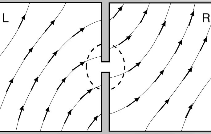
FIG. 1.: A weak link between two bulk superfluids, $L$ and $R$. The arrows denote the $\hat{{\bf{n}}}$ vector of ³He-B. The dashed line divides the liquid into a mesoscopic region (inside) and a macroscopic region (outside).

We consider the system to consist of a mesoscopic region at the junction and a macroscopic region outside. There can be considerable variation of the soft degrees of freedom in the macroscopic region, as illustrated for the $\hat{{\bf{n}}}$ vector in Fig. 1. The mesoscopic region is chosen sufficiently small so that (i) both $\phi$ and $R_{\mu i}$ are effectively constants at the macroscopic-mesoscopic border, and (ii) the weak interactions affecting $\phi$ and $R_{\mu i}$ can be neglected in the mesoscopic region. The size of the mesoscopic region is limited from below by the condition that the bulk form of the order parameter (1) has to be valid in the macroscopic region. Thus the size of the mesoscopic region has to be large in comparison to both the superfluid coherence length $\xi_{0}\approx 10$ nm and the size of the aperture. The mesoscopic region can also be chosen to cover several apertures.

The rotation matrices and the phases on the left ($L$) and right ($R$) sides are generally different. Their values at the macroscopic-mesoscopic border are denoted by $R_{\mu i}^{L,R}$ and $\phi^{L,R}$. The most general form for the Josephson coupling energy associated with the weak link is given by

$$F_{\rm J}=F_{\rm J}(\phi^{L},\phi^{R},R_{\mu i}^{L},R_{\nu j}^{R}).$$ (2)

However, due to global phase invariance there can really be only a dependence on the phase difference $\phi\equiv\phi^{R}-\phi^{L}$. In addition, if we assume the intervening wall to be magnetically inactive, then we should have invariance with respect to global spin rotations as well. This means that the energy can only depend on the product of the rotation matrices, or the quantities $\psi_{ij}=R_{\mu i}^{L}R_{\mu j}^{R}$, so that

$$F_{\rm J}=F_{\rm J}(\phi,R_{\mu i}^{L}R_{\mu j}^{R}).$$ (3)

Using the functional $F_{\rm J}$ (3) one can now calculate two conserved currents. Firstly, the mass current through the aperture is given by

$$J=\frac{2m_{3}}{\hbar}\frac{\partial F_{\rm J}}{\partial\phi}.$$ (4)

See, for example, Ref. [18]. Secondly, due to the different spin-orbit rotation matrices on the two sides, there is also a spin current flowing through the aperture. Likewise, this is obtained from $F_{\rm{J}}$ by differentiation:

$$J^{\rm{spin}}_{\gamma}=\epsilon_{\alpha\beta\gamma}R_{\alpha i}^{L}R_{\beta j}^{R}\frac{\partial F_{\rm J}}{\partial(R_{\mu i}^{L}R_{\mu j}^{R})}.$$ (5)

This can be seen by replacing $\psi_{ij}$ in (3) by $R_{\alpha i}^{L}R_{\beta j}^{R}R_{\alpha\beta}$ with the relative rotation $R_{\alpha\beta}=\delta_{\alpha\beta}+\epsilon_{\alpha\beta\gamma}\delta\theta_{\gamma}$, and identifying $\delta F_{\rm J}=J_{\gamma}^{\rm{spin}}\delta\theta_{\gamma}+O(\delta\theta_{\gamma}^{2})$ [19].

The energy and the currents also satisfy some other symmetry relations. For example, assuming invariance with respect to time reversal, we have $F_{\rm J}(-\phi,\psi_{ij})=F_{\rm J}(\phi,\psi_{ij})$. As a consequence $J(-\phi,\psi_{ij})=-J(\phi,\psi_{ij})$ and $J^{\rm{spin}}_{\gamma}(-\phi,\psi_{ij})=J^{\rm{spin}}_{\gamma}(\phi,\psi_{ij})$. Also, since the phase factor $\exp({\mathrm{i}}\phi)$ is defined only modulo $2\pi$, we have $F_{\rm J}(\phi+2\pi,\psi_{ij})=F_{\rm J}(\phi,\psi_{ij})$. Here we must keep in mind that in a long junction $F_{\rm J}$ is not a single-valued function. Analogously, there is periodicity with respect to the rotation angle, which is automatically contained in the form of Eq. (2), since $R_{\mu i}(\hat{{\bf{n}}},\theta+2\pi)=R_{\mu i}(\hat{{\bf{n}}},\theta)$.

The functional form of $F_{\rm J}$ (3) can be restricted further if we assume some additional symmetries. For example, if the aperture is symmetric under a parity operation, we have $F_{\rm J}(\phi,\psi_{ji})=F_{\rm J}(\phi,\psi_{ij})$ and thus $J_{\gamma}^{\rm{spin}}(\phi,\psi_{ji})=-J_{\gamma}^{\rm{spin}}(\phi,\psi_{ij})$. If the aperture has full “orthorhombic” symmetry $\frac{2}{m}\frac{2}{m}\frac{2}{m}$, then $F_{\rm J}$ can only depend on the rotation matrices through $\psi_{xx}$, $\psi_{yy}$, and $\psi_{zz}$. From here on we fix the $z$ coordinate to be along the axis of the weak link. Now, if the twofold rotation symmetry around $z$ is replaced by a fourfold symmetry ($\frac{4}{m}\frac{2}{m}\frac{2}{m}$), then an exchange of $\psi_{xx}$ and $\psi_{yy}$ must not affect $F_{\rm J}$. Finally, if the rotation symmetry around $z$ is continuous ($\frac{\infty}{m}\frac{2}{m}$), the dependence can only be through $\psi_{zz}$ and the invariant combination $\psi_{xx}+\psi_{yy}$, that is

$$F_{\rm J}=F_{\rm J}(\phi,R_{\mu x}^{L}R_{\mu x}^{R}+R_{\mu y}^{L}R_{\mu y}^{R},R_{\mu z}^{L}R_{\mu z}^{R}).$$ (6)

Close to $T_{\rm c}$ the amplitude $\Delta$ of the order parameter (1) approaches zero, so that we can expand $F_{\rm J}(A_{\mu i}^{L},A_{\nu j}^{R})$ in powers of $\Delta$. In order to be consistent with Eq. (6), the leading order term in the expansion must be

$$F_{\rm J}=-[\alpha R_{\mu z}^{L}R_{\mu z}^{R}+\beta(R_{\mu x}^{L}R_{\mu x}^{R}+R_{\mu y}^{L}R_{\mu y}^{R})]\cos\phi,$$ (7)

where $\alpha$ and $\beta$ are some real valued phenomenological constants. In Ref. [11] this was introduced as the Josephson energy of the tunneling model, but as the derivation above shows, it is more general. The tunneling barrier for ³He was first considered in Ref. [20].

In order to further determine the functional $F_{\rm J}$ (3,6,7) it is necessary to do a calculation in the mesoscopic region. This is discussed in the following sections III-VI.

III Quasiclassical theory

We use the quasiclassical theory of Fermi liquids [21] to calculate $F_{\rm J}$ (3) for a pinhole aperture. Here we present the theory only in the depth needed for the following.

The central quantity is the quasiclassical propagator $\breve{g}$. In the stationary case which we are considering this can be written as $\breve{g}({\hat{{\bf{k}}}},{\bf{r}},\epsilon_{m})$, where ${\bf{r}}$ denotes spatial position, ${\hat{{\bf{k}}}}$ parametrizes a position on the Fermi surface, and $\epsilon_{m}=\pi k_{\mathrm{B}}T(2m+1)$ are the Matsubara energies. The propagator is determined by the Eilenberger equation and the normalization condition

$$[{\mathrm{i}}\epsilon_{m}\breve{\tau}_{3}-\breve{\sigma},\breve{g}]+{\mathrm{i}}\hbar v_{\mathrm{F}}{\hat{{\bf{k}}}}\cdot\nabla_{{\bf{r}}}\breve{g} = 0$$ (8)

$$\breve{g}\breve{g} = -\breve{1}.$$ (9)

Equation (8) can be interpreted as describing transport of quasiparticle wave packets which travel on classical trajectories with the Fermi velocity ${\bf{v}}_{\rm{F}}=v_{\mathrm{F}}{\hat{{\bf{k}}}}$. The propagator $\breve{g}$ as well as the self-energy $\breve{\sigma}({\hat{{\bf{k}}}},{\bf{r}})$ are $4\times 4$ matrices, reflecting the spin and particle-hole degrees of freedom of a quasiparticle; the matrices $\breve{\tau}_{i}$ $(i=1,2,3)$ are the Pauli matrices in the particle-hole space.

The $2\times 2$ spin blocks of $\breve{g}$ can be decomposed into scalar and vector components as

$$\breve{g}=\left[\begin{array}[]{cc}g+{\bf{g}}\cdot\underline{\mathchoice{{\hbox{\boldmath$\displaystyle\sigma$}}}{{\hbox{\boldmath$\textstyle\sigma$}}}{{\hbox{\boldmath$\scriptstyle\sigma$}}}{{\hbox{\boldmath$\scriptscriptstyle\sigma$}}}}&(f+{\bf{f}}\cdot\underline{\mathchoice{{\hbox{\boldmath$\displaystyle\sigma$}}}{{\hbox{\boldmath$\textstyle\sigma$}}}{{\hbox{\boldmath$\scriptstyle\sigma$}}}{{\hbox{\boldmath$\scriptscriptstyle\sigma$}}}}){\mathrm{i}}\underline{\sigma}_{2}\\ {\mathrm{i}}\underline{\sigma}_{2}(\tilde{f}+\tilde{\bf{f}}\cdot\underline{\mathchoice{{\hbox{\boldmath$\displaystyle\sigma$}}}{{\hbox{\boldmath$\textstyle\sigma$}}}{{\hbox{\boldmath$\scriptstyle\sigma$}}}{{\hbox{\boldmath$\scriptscriptstyle\sigma$}}}})&\tilde{g}-\underline{\sigma}_{2}\tilde{\bf{g}}\cdot\underline{\mathchoice{{\hbox{\boldmath$\displaystyle\sigma$}}}{{\hbox{\boldmath$\textstyle\sigma$}}}{{\hbox{\boldmath$\scriptstyle\sigma$}}}{{\hbox{\boldmath$\scriptscriptstyle\sigma$}}}}\,\underline{\sigma}_{2}\end{array}\right],$$ (10)

where $\underline{\mathchoice{{\hbox{\boldmath$\displaystyle\sigma$}}}{{\hbox{\boldmath$\textstyle\sigma$}}}{{\hbox{\boldmath$\scriptstyle\sigma$}}}{{\hbox{\boldmath$\scriptscriptstyle\sigma$}}}}=\hat{{\bf{x}}}\underline{\sigma}_{1}+\hat{{\bf{y}}}\underline{\sigma}_{2}+\hat{{\bf{z}}}\underline{\sigma}_{3}$, and $\underline{\sigma}_{i}$ $(i=1,2,3)$ are the spin-space Pauli matrices. The self-energy $\breve{\sigma}$ is written similarly

$$\breve{\sigma}=\left[\begin{array}[]{cc}\nu+\mathchoice{{\hbox{\boldmath$\displaystyle\nu$}}}{{\hbox{\boldmath$\textstyle\nu$}}}{{\hbox{\boldmath$\scriptstyle\nu$}}}{{\hbox{\boldmath$\scriptscriptstyle\nu$}}}\cdot\underline{\mathchoice{{\hbox{\boldmath$\displaystyle\sigma$}}}{{\hbox{\boldmath$\textstyle\sigma$}}}{{\hbox{\boldmath$\scriptstyle\sigma$}}}{{\hbox{\boldmath$\scriptscriptstyle\sigma$}}}}&\mathchoice{{\hbox{\boldmath$\displaystyle\Delta$}}}{{\hbox{\boldmath$\textstyle\Delta$}}}{{\hbox{\boldmath$\scriptstyle\Delta$}}}{{\hbox{\boldmath$\scriptscriptstyle\Delta$}}}\cdot\underline{\mathchoice{{\hbox{\boldmath$\displaystyle\sigma$}}}{{\hbox{\boldmath$\textstyle\sigma$}}}{{\hbox{\boldmath$\scriptstyle\sigma$}}}{{\hbox{\boldmath$\scriptscriptstyle\sigma$}}}}{\mathrm{i}}\underline{\sigma}_{2}\\ {\mathrm{i}}\underline{\sigma}_{2}\mathchoice{{\hbox{\boldmath$\displaystyle\Delta$}}}{{\hbox{\boldmath$\textstyle\Delta$}}}{{\hbox{\boldmath$\scriptstyle\Delta$}}}{{\hbox{\boldmath$\scriptscriptstyle\Delta$}}}^{*}\cdot\underline{\mathchoice{{\hbox{\boldmath$\displaystyle\sigma$}}}{{\hbox{\boldmath$\textstyle\sigma$}}}{{\hbox{\boldmath$\scriptstyle\sigma$}}}{{\hbox{\boldmath$\scriptscriptstyle\sigma$}}}}&\tilde{\nu}-\underline{\sigma}_{2}\tilde{\mathchoice{{\hbox{\boldmath$\displaystyle\nu$}}}{{\hbox{\boldmath$\textstyle\nu$}}}{{\hbox{\boldmath$\scriptstyle\nu$}}}{{\hbox{\boldmath$\scriptscriptstyle\nu$}}}}\cdot\underline{\mathchoice{{\hbox{\boldmath$\displaystyle\sigma$}}}{{\hbox{\boldmath$\textstyle\sigma$}}}{{\hbox{\boldmath$\scriptstyle\sigma$}}}{{\hbox{\boldmath$\scriptscriptstyle\sigma$}}}}\,\underline{\sigma}_{2}\end{array}\right].$$ (11)

Here the off-diagonal terms contain the $p$-wave pairing interaction in the form of the gap vector $\Delta_{\mu}({\hat{{\bf{k}}}},{\bf{r}})=A_{\mu i}({\bf{r}})\hat{k}_{i}$. This is determined by the self-consistency equation

$$\pi k_{\mathrm{B}}T \sum_{m}\left[\frac{\mathchoice{{\hbox{\boldmath$\displaystyle\Delta$}}}{{\hbox{\boldmath$\textstyle\Delta$}}}{{\hbox{\boldmath$\scriptstyle\Delta$}}}{{\hbox{\boldmath$\scriptscriptstyle\Delta$}}}}{|\epsilon_{m}|}-3\int\frac{{\mathrm{d}}\Omega_{{\hat{{\bf{k}}}}^{\prime}}}{4\pi}{\bf{f}}({\hat{{\bf{k}}}}^{\prime},{\bf{r}},\epsilon_{m})({\hat{{\bf{k}}}}^{\prime}\cdot{\hat{{\bf{k}}}})\right]$$ (13)

$$+\mathchoice{{\hbox{\boldmath$\displaystyle\Delta$}}}{{\hbox{\boldmath$\textstyle\Delta$}}}{{\hbox{\boldmath$\scriptstyle\Delta$}}}{{\hbox{\boldmath$\scriptscriptstyle\Delta$}}}\ln\frac{T}{T_{\rm c}}={\bf{0}},$$

where $T_{\rm c}$ is the superfluid transition temperature. This form is valid in the weak coupling approximation, where the quasiparticle-quasiparticle scattering is neglected. The diagonal components $\nu,\tilde{\nu}$ and $\mathchoice{{\hbox{\boldmath$\displaystyle\nu$}}}{{\hbox{\boldmath$\textstyle\nu$}}}{{\hbox{\boldmath$\scriptstyle\nu$}}}{{\hbox{\boldmath$\scriptscriptstyle\nu$}}},\tilde{\mathchoice{{\hbox{\boldmath$\displaystyle\nu$}}}{{\hbox{\boldmath$\textstyle\nu$}}}{{\hbox{\boldmath$\scriptstyle\nu$}}}{{\hbox{\boldmath$\scriptscriptstyle\nu$}}}}$ are the “molecular field” self-energies arising from redistributions of quasiparticles. The scalar parameters $\nu$ and $\tilde{\nu}$ arise in response to mass currents, and they turn out to be negligible as will be argued in Sec. IV. The (real valued) vector parameters $\textstyle\nu$ and $\tilde{\mathchoice{{\hbox{\boldmath$\displaystyle\nu$}}}{{\hbox{\boldmath$\textstyle\nu$}}}{{\hbox{\boldmath$\scriptstyle\nu$}}}{{\hbox{\boldmath$\scriptscriptstyle\nu$}}}}$ describe the response to a magnetic field or spin currents. As discussed above, the magnetic field can be neglected in the mesoscopic region. In contrast, there are always rather strong spin currents flowing along surfaces in ³He-B [22]. These have to be taken into account with the self-consistency relation ($\tilde{\mathchoice{{\hbox{\boldmath$\displaystyle\nu$}}}{{\hbox{\boldmath$\textstyle\nu$}}}{{\hbox{\boldmath$\scriptstyle\nu$}}}{{\hbox{\boldmath$\scriptscriptstyle\nu$}}}}=-\mathchoice{{\hbox{\boldmath$\displaystyle\nu$}}}{{\hbox{\boldmath$\textstyle\nu$}}}{{\hbox{\boldmath$\scriptstyle\nu$}}}{{\hbox{\boldmath$\scriptscriptstyle\nu$}}}$)

$$\mathchoice{{\hbox{\boldmath$\displaystyle\nu$}}}{{\hbox{\boldmath$\textstyle\nu$}}}{{\hbox{\boldmath$\scriptstyle\nu$}}}{{\hbox{\boldmath$\scriptscriptstyle\nu$}}}({\hat{{\bf{k}}}},{\bf{r}})=\pi k_{\mathrm{B}}T\sum_{m}\int\frac{{\mathrm{d}}\Omega_{{\hat{{\bf{k}}}}^{\prime}}}{4\pi}A^{a}({\hat{{\bf{k}}}}\cdot{\hat{{\bf{k}}}}^{\prime}){\bf{g}}({\hat{{\bf{k}}}}^{\prime},{\bf{r}},\epsilon_{m}).$$ (14)

Here $A^{a}(x)=\sum_{l=0}^{\infty}F^{a}_{l}[1+F^{a}_{l}/(2l+1)]^{-1}P_{l}(x)$, $P_{l}$ are the Legendre polynomials, and all terms with even $l$ drop out due to symmetries.

For our purposes the most important physical quantities to be evaluated from $\breve{g}$ are the mass supercurrent

$${\bf{j}}({\bf{r}})=2m_{3}v_{\mathrm{F}}N(0)\pi k_{\mathrm{B}}T\sum_{m}\int\frac{{\mathrm{d}}\Omega_{\hat{{\bf{k}}}}}{4\pi}{\hat{{\bf{k}}}}g({\hat{{\bf{k}}}},{\bf{r}},\epsilon_{m})$$ (15)

and the spin supercurrent

$${\bf{j}}^{\rm{spin}}_{\gamma}({\bf{r}})=\hbar v_{\mathrm{F}}N(0)\pi k_{\mathrm{B}}T\sum_{m}\int\frac{{\mathrm{d}}\Omega_{\hat{{\bf{k}}}}}{4\pi}{\hat{{\bf{k}}}}g_{\gamma}({\hat{{\bf{k}}}},{\bf{r}},\epsilon_{m}).$$ (16)

Here $N(0)=m^{*}{}^{2}v_{\mathrm{F}}/(2\pi^{2}\hbar^{3})$ is the one-spin normal-state density of states at the Fermi surface, where $m^{*}=m_{3}(1+F_{1}^{s}/3)$ is the effective quasiparticle mass, $m_{3}$ being the mass of a bare ³He atom. The superfluid coherence length is defined by $\xi_{0}=\hbar v_{\mathrm{F}}/(2\pi k_{\mathrm{B}}T_{\rm c})$. For $F_{1}^{s}$, $v_{\mathrm{F}}$, $T_{\rm c}$ and other pressure dependent quantities we use the vapor pressure values whenever needed. In Eq. (14) we assume $F_{l}^{a}=0$ for all odd $l\geq 3$. Since the parameter $F^{a}_{1}$ is not well known, we usually set it to zero also, but values in the range $-1...0$ have been tested.

IV The pinhole problem

Consider the case of a single pinhole in a thin wall separating two volumes of ³He-B — the situation of Fig. 2.

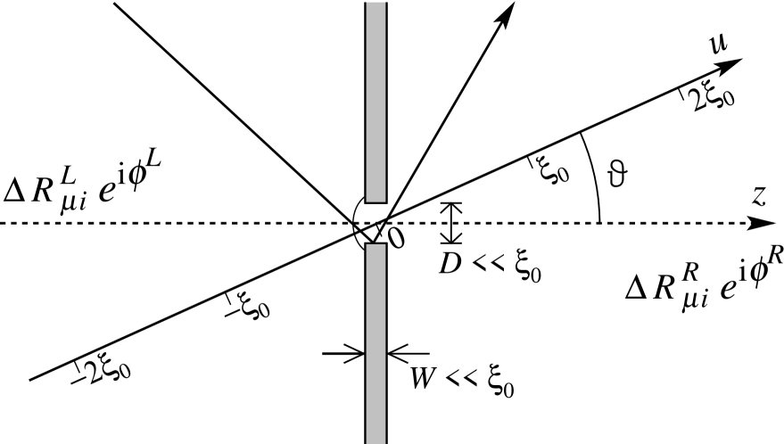
FIG. 2.: The mesoscopic region (Fig. 1) for a pinhole. Two quasiparticle trajectories are shown. The coordinate $u$ is plotted along the straight transmitting trajectory. The arch on the left hand side of the pinhole denotes an imaginary surface that is used to close the pinhole (Sec. V). The diameter $D$ of the pinhole and the thickness of the wall $W$ are assumed small in comparison to $\xi_{0}$.

The hole can be thought of as a pinhole (i.e. “very small”) and still be treated quasiclassically, if its dimensions (diameter $D$ and wall thickness $W$) satisfy $\xi_{0}\gg D,W\gg\lambda_{\rm{F}}$, where $\lambda_{\rm{F}}$ is the Fermi wavelength. In addition ³He is in the pure limit, where the mean free path of quasiparticles $l\gg\xi_{0}$. Usually one further assumes that $W\ll D$ so that scattering in the aperture itself can be neglected. We allow for a finite $W/D$ and thus consider also deflected trajectories of the form shown in Fig. 2. The pinhole limit was first considered within the quasiclassical theory by Kulik and Omel’yanchuk in the case of $s$-wave superconducting microbridges [15]. Several previous calculations for the spin-triplet case of ³He also exist [10, 11, 16, 23, 24, 25, 26]. For another type of quasiclassical Josephson model, see Ref. [27].

What makes the pinhole case attractive is that no self-consistent calculation of the order parameter in the aperture is needed. More precisely, the leading term in the coupling energy $F_{\rm J}$ is on the order of the superfluid condensation energy in the volume $D^{2}\xi_{0}$. This effective volume is large compared to the volume ($\sim D^{3}$ or $WD^{2}$) of the pinhole. The leading term in $F_{\rm J}$ (and thus also the corresponding terms in the currents) can be computed using $\breve{\sigma}$ (11) that is calculated for a planar wall without the pinhole. There is a correction $\propto D^{2}$ to $\breve{\sigma}$, but because of the stationarity of the energy functional with respect to $\breve{\sigma}$, this affects $F_{\rm J}$ only in the order $\propto D^{4}/\xi_{0}$, which is negligible for a pinhole. Therefore we can use the order parameter profiles calculated for a planar wall.

Determining the suppression of the order parameter $\textstyle\Delta$ at the wall is thus the first step needed for our calculation. In the absence of mass currents and magnetic scattering it is sufficient to consider the parametrization

$$\mathchoice{{\hbox{\boldmath$\displaystyle\Delta$}}}{{\hbox{\boldmath$\textstyle\Delta$}}}{{\hbox{\boldmath$\scriptstyle\Delta$}}}{{\hbox{\boldmath$\scriptscriptstyle\Delta$}}}^{(0)}({\hat{{\bf{k}}}},z)=[\Delta_{\perp}(z)\hat{{\bf{z}}}\hat{{\bf{z}}}+\Delta_{\parallel}(z)(\hat{{\bf{x}}}\hat{{\bf{x}}}+\hat{{\bf{y}}}\hat{{\bf{y}}})]\cdot{\hat{{\bf{k}}}},$$ (17)

where $\hat{{\bf{z}}}$ is perpendicular to the wall. The gap functions $\Delta_{\perp}(z)$ and $\Delta_{\parallel}(z)$, which are real valued, are calculated self-consistently as explained in Ref. [22]. For $\breve{g}$ we use the “randomly oriented mirror” (ROM) boundary condition at a specular or a diffusive surface [25]. The numerical calculation of $\breve{g}$ is described in Sect. IV. Our results for $\Delta_{\perp}(z)$ and $\Delta_{\parallel}(z)$ are similar to those found previously with ROM and other surface models [22, 25, 26, 28, 29, 30, 31]. In order to incorporate different phases and spin-orbit rotations on the two sides we write

$$\mathchoice{{\hbox{\boldmath$\displaystyle\Delta$}}}{{\hbox{\boldmath$\textstyle\Delta$}}}{{\hbox{\boldmath$\scriptstyle\Delta$}}}{{\hbox{\boldmath$\scriptscriptstyle\Delta$}}}({\hat{{\bf{k}}}},z)=\left\{\begin{array}[]{ll}\exp({\mathrm{i}}\phi^{L})\tensor{R}^{L}\!\cdot\mathchoice{{\hbox{\boldmath$\displaystyle\Delta$}}}{{\hbox{\boldmath$\textstyle\Delta$}}}{{\hbox{\boldmath$\scriptstyle\Delta$}}}{{\hbox{\boldmath$\scriptscriptstyle\Delta$}}}^{(0)}({\hat{{\bf{k}}}},z)&{\rm{for}}~{}z<0\\ \exp({\mathrm{i}}\phi^{R})\tensor{R}^{R}\!\cdot\mathchoice{{\hbox{\boldmath$\displaystyle\Delta$}}}{{\hbox{\boldmath$\textstyle\Delta$}}}{{\hbox{\boldmath$\scriptstyle\Delta$}}}{{\hbox{\boldmath$\scriptscriptstyle\Delta$}}}^{(0)}({\hat{{\bf{k}}}},z)&{\rm{for}}~{}z>0\\ \end{array}\right..$$ (18)

The thin wall is located at $z=0$ and $\mathchoice{{\hbox{\boldmath$\displaystyle\Delta$}}}{{\hbox{\boldmath$\textstyle\Delta$}}}{{\hbox{\boldmath$\scriptstyle\Delta$}}}{{\hbox{\boldmath$\scriptscriptstyle\Delta$}}}^{(0)}$ (17) is assumed to be symmetric: $\Delta_{\perp}(-z)=\Delta_{\perp}(z)$ and $\Delta_{\parallel}(-z)=\Delta_{\parallel}(z)$.

V Energy functional

Here we derive a general quasiclassical expression for the Josephson coupling energy in a pinhole. The derivation follows closely the lines of a quasiclassical treatment of impurities in ³He or superconductors [32, 33]. We start from an expression for the energy difference between states with one impurity and no impurity, $\breve{V}$ being the impurity potential [21, 34]. For a small spatial range of $\breve{V}$, the self-energy $\breve{\Sigma}$ can be assumed to be unchanged by it, and we get [32]

$$\delta\Omega^{\rm tot}=-\frac{1}{2}\mathop{\mathrm{Tr}}[\ln(-\breve{G}_{0}^{-1}+\breve{\Sigma}+\breve{V})-\ln(-\breve{G}_{0}^{-1}+\breve{\Sigma})].$$ (19)

The trace operation $\mathop{\mathrm{Tr}}$ is defined as

$$\mathop{\mathrm{Tr}}\breve{F}=k_{\mathrm{B}}T\sum_{m}\int\frac{{\mathrm{d}}^{3}k}{(2\pi)^{3}}{\mathop{\mathrm{Tr}}}_{4}\breve{F}({\bf{k}},{\bf{k}},\epsilon_{m}),$$ (20)

where $\mathop{\mathrm{Tr}}_{4}$ denotes the trace of the $4\times 4$ Nambu matrix $\breve{F}$. To eliminate the logarithm, we may apply some form of the “$\lambda$-trick” [35]. We choose to integrate over the strength of $\breve{V}$ by making the substitution $\breve{V}\rightarrow\lambda\breve{V}$ and writing

$$\delta\Omega^{\rm tot} = \frac{1}{2}\mathop{\mathrm{Tr}}\int_{0}^{1}\frac{{\mathrm{d}}\lambda}{\lambda}(\breve{G}_{0}^{-1}-\breve{\Sigma}-\lambda\breve{V})^{-1}\lambda\breve{V}$$ (21)

$$= \frac{1}{2}\mathop{\mathrm{Tr}}\int_{0}^{1}\frac{{\mathrm{d}}\lambda}{\lambda}\breve{G}_{1}\breve{T}_{\lambda}.$$ (22)

The latter equality follows from a formal application of the $t$-matrix equation $\breve{T}_{\lambda}=\lambda\breve{V}+\breve{T}_{\lambda}\breve{G}_{1}\lambda\breve{V}$ and the relation $\breve{G}=\breve{G}_{1}+\breve{G}_{1}\breve{T}_{\lambda}\breve{G}_{1}$. Here $\breve{G}=(\breve{G}_{0}^{-1}-\breve{\Sigma}-\lambda\breve{V})^{-1}$ gives the full propagator in the presence of an impurity scattering potential. The intermediate Green’s function $\breve{G}_{1}$ corresponds to a quasiclassical $\breve{g}_{1}$ which has no discontinuity at the impurity. Equation (21) is now in a form where the propagator can be $|{\bf k}|$-integrated directly. However, to avoid a divergence in the Matsubara summation, we have to subtract from (21) the normal-state contribution $\delta\Omega^{\rm N}$, obtained by setting $\breve{\Sigma}=\breve{\Sigma}^{\rm N}$ in (19). We define $\delta\Omega=\delta\Omega^{\rm tot}-\delta\Omega^{\rm N}$ and transform this to the quasiclassical form

$$\delta\Omega=\frac{1}{2} \hbar v_{\mathrm{F}}N(0)\pi k_{\mathrm{B}}T\sum_{m}\int\frac{{\mathrm{d}}\Omega_{\hat{{\bf{k}}}}}{4\pi}\int_{0}^{1}\frac{{\mathrm{d}}\lambda}{\lambda}$$ (23)

$$\times{\mathop{\mathrm{Tr}}}_{4} [\breve{g}_{1}({\hat{{\bf{k}}}},{\bf{r}}_{\rm{imp}},\epsilon_{m})\breve{t}_{\lambda}({\hat{{\bf{k}}}},{\hat{{\bf{k}}}},\epsilon_{m})$$ (25)

$$-\breve{g}^{\rm N}_{1}({\hat{{\bf{k}}}},{\bf{r}}_{\rm{imp}},\epsilon_{m})\breve{t}^{\rm N}_{\lambda}({\hat{{\bf{k}}}},{\hat{{\bf{k}}}},\epsilon_{m})],$$

where ${\bf{r}}_{\rm{imp}}$ is the location of the impurity and $\breve{t}_{\lambda}({\hat{{\bf{k}}}},{\hat{{\bf{k}}}},\epsilon_{m})$ is the forward-scattering part of the $t$ matrix, which is obtained by solving

$$\breve{t}_{\lambda}({\hat{{\bf{k}}}},{\hat{{\bf{k}}}}^{\prime},\epsilon_{m}) = \lambda\breve{v}({\hat{{\bf{k}}}},{\hat{{\bf{k}}}}^{\prime})+\lambda\pi N(0)\int\frac{{\mathrm{d}}\Omega_{{\hat{{\bf{k}}}}^{\prime\prime}}}{4\pi}\breve{v}({\hat{{\bf{k}}}},{\hat{{\bf{k}}}}^{\prime\prime})$$ (27)

$$\times\breve{g}_{1}({\hat{{\bf{k}}}}^{\prime\prime},{\bf{r}}_{\rm{imp}},\epsilon_{m})\breve{t}_{\lambda}({\hat{{\bf{k}}}}^{\prime\prime},{\hat{{\bf{k}}}}^{\prime},\epsilon_{m}).$$

The energy formula (23) is simpler to use than those in Refs. [32, 33], since it does not involve an integration over ${\bf{r}}$. More importantly, $\breve{g}_{1}$ is constant in the $\lambda$ integration.

Now we specialize the above approach to the pinhole problem. The coupling energy $F_{\rm J}$ we wish to know is, by definition, the difference in energies between an open pinhole and a blocked pinhole. It should be irrelevant how the hole is blocked as long as the transmission of quasiparticles is prevented: changing the type of blockage should only change some constant terms in the energy, which do not depend on the soft degrees of freedom in (3). We choose to block the pinhole by a surface just on the left hand side of it (Fig. 2). This surface is now considered as the “impurity” in Eqs. (19-27). The coupling energy is then equal to $\delta\Omega$ (23) except for a minus sign: $F_{\rm J}=-\delta\Omega$. The intermediate $\breve{g}_{1}$ is the exact propagator that is calculated for an open pinhole, and we drop the subindex 1 from here on.

The simplest choice for the blocking wall is a specularly scattering surface. It corresponds to a delta-function scattering potential ${\mathcal{V}}\delta(\hat{\bf l}\cdot{{\bf{r}}})$ for the (infinitesimal piece of) flat surface $\hat{\bf l}\cdot{\bf{r}}=0$ in the limit ${\mathcal{V}}\rightarrow\infty$. The $t$ matrix of this type of impurity is of particularly simple form [28, 21]

$$\breve{t}_{\lambda} ({\hat{{\bf{k}}}},{\hat{{\bf{k}}}}^{\prime},\epsilon_{m})=$$ (29)

$$\frac{2v_{\mathrm{F}}|{\hat{{\bf{k}}}}\cdot\hat{\bf l}|\lambda{\mathcal{V}}{\mathrm{d}}A\delta^{(2)}_{{\bf k}_{\parallel},{\bf k}^{\prime}_{\parallel}}}{2v_{\mathrm{F}}|{\hat{{\bf{k}}}}\cdot\hat{\bf l}|-\lambda{\mathcal{V}}[\breve{g}({\hat{{\bf{k}}}},{\bf{r}}_{\rm{imp}},\epsilon_{m})+\breve{g}(\underline{{\hat{{\bf{k}}}}},{\bf{r}}_{\rm{imp}},\epsilon_{m})]},$$

where ${\mathrm{d}}A$ is an area element ($\lambda_{F}^{2}\ll{\mathrm{d}}A\ll\xi_{0}^{2}$) of the blocking piece of wall with normal $\hat{\bf l}$. The component of ${\hat{{\bf{k}}}}$ parallel to this wall is denoted by ${\bf k}_{\parallel}={\hat{{\bf{k}}}}-({\hat{{\bf{k}}}}\cdot\hat{\bf l})\hat{\bf l}$, and $\underline{{\hat{{\bf{k}}}}}={\hat{{\bf{k}}}}-2({\hat{{\bf{k}}}}\cdot\hat{\bf l})\hat{\bf l}$ is the mirror-reflected direction. We insert $\breve{t}_{\lambda}$ (29) into $\delta\Omega$ (23) and integrate over the blocking surface. Performing also the $\lambda$-integration, we find

$$F_{\rm J}( {\mathcal{V}})=-\frac{1}{2}\hbar v_{\mathrm{F}}N(0)\pi k_{\mathrm{B}}T\int{\mathrm{d}}A\sum_{m}\int\frac{{\mathrm{d}}\Omega_{\hat{{\bf{k}}}}}{4\pi}|{\hat{{\bf{k}}}}\cdot\hat{\bf l}|{\mathop{\mathrm{Tr}}}_{4}$$ (31)

$$\times\ln\frac{2v_{\mathrm{F}}|{\hat{{\bf{k}}}}\cdot\hat{\bf l}|-{\mathcal{V}}[\breve{g}({\hat{{\bf{k}}}},{\bf{r}}_{\rm{imp}},\epsilon_{m})+\breve{g}(\underline{{\hat{{\bf{k}}}}},{\bf{r}}_{\rm{imp}},\epsilon_{m})]}{2v_{\mathrm{F}}|{\hat{{\bf{k}}}}\cdot\hat{\bf l}|+2{\mathrm{i}}{\mathcal{V}}\breve{\tau}_{3}\mathop{\rm{Sgn}}(\epsilon_{m})}$$

where the normal-state propagator $\breve{g}^{\rm N}={\mathrm{i}}\breve{\tau}_{3}\mathop{\rm{Sgn}}(\epsilon_{m})$ was used. Next we take the limit $\mathcal{V}\rightarrow\infty$ and use the general properties ${\mathop{\mathrm{Tr}}}_{4}\ln\breve{A}=\ln{\mathop{\rm{Det}}}_{4}\breve{A}$ and ${\mathop{\rm{Det}}}_{4}\breve{A}\breve{B}={\mathop{\rm{Det}}}_{4}\breve{A}{\mathop{\rm{Det}}}_{4}\breve{B}$, noting further that ${\mathop{\rm{Det}}}_{4}[{\mathrm{i}}\breve{\tau}_{3}\mathop{\rm{Sgn}}(\epsilon_{m})]=1$. All trajectories that do not pass through the hole in the absence of the blockade can be neglected, and thus the integration over the surface $A$ can be transformed to one over the cross section (of area $A_{o}$) of the hole. This leads to the general pinhole energy functional

$$F_{\rm{J}} =-\frac{1}{2}A_{o}\hbar v_{\mathrm{F}}N(0)\pi k_{\mathrm{B}}T{\sum_{m}}\int\frac{{\mathrm{d}}\Omega_{\hat{{\bf{k}}}}}{4\pi}|\hat{k}_{z}|$$ (33)

$$\times\left\langle\ln\left\{{\mathop{\rm{Det}}}_{4}\frac{1}{2}[\breve{g}({\hat{{\bf{k}}}},{\bf 0}^{L},\epsilon_{m})+\breve{g}(\underline{{\hat{{\bf{k}}}}},{\bf 0}^{L},\epsilon_{m})]\right\}\right\rangle,$$

where $\hat{k}_{z}={\hat{{\bf{k}}}}\cdot\hat{{\bf{z}}}$, the brackets $\langle\dots\rangle$ denote average over the trajectories (at fixed ${\hat{{\bf{k}}}}$) that hit the area $A_{o}$ of the pinhole ($A_{o}=\pi D^{2}/4$ for a circular hole), and ${\bf 0}^{L}$ denotes the location immediately on the left hand side of the hole.

The coupling energy (33) depends on the shape of the blocking wall only through the directions of the reflected momenta $\underline{{\hat{{\bf{k}}}}}={\hat{{\bf{k}}}}-2({\hat{{\bf{k}}}}\cdot\hat{\bf l})\hat{\bf l}$. Because the surface can be chosen in different ways, there is a lot of freedom in choosing the reflected momenta. A particularly simple choice is retroreflection: $\underline{{\hat{{\bf{k}}}}}=-{\hat{{\bf{k}}}}$. This can be achieved, for example, by a semispherical blocking surface of radius $R$ satisfying $\xi_{0}\gg R\gg D$, centered at the pinhole. This choice can simplify practical calculations considerably, since one can use symmetries effectively. After this one may, for example, calculate the determinant by using ${\mathrm{Det}}_{4}(\breve{g}_{1}+\breve{g}_{2})=[{\mathrm{Det}}_{4}(-2\breve{1}+\{\breve{g}_{1},\breve{g}_{2}\})]^{1/2}$.

The choice to block the surface on the left hand side was arbitrary and the blocking could equally well be done on the right hand side. The reason for not blocking in the middle of the hole is that there may be scattering taking place there. For example, a quasiparticle may hit the wall inside of the hole and be deflected (Fig. 2). In general this causes $\breve{g}$ to be discontinuous at the hole, and in order to give an unambiguous prescription for $F_{\rm J}$ (33), one has to specify one of the sides. If there is no scattering in the pinhole ($W/D=0$), the propagator is continuous and the energy functional can be evaluated in the middle of the hole. In the absence of scattering also the average $\langle\dots\rangle$ in $F_{\rm{J}}$ (33) is trivial and can be dropped.

Apart from the assumption of a pinhole aperture, the energy functional (33) is very general. Below we shall apply it for the special case of ³He-B.

VI Pinhole calculation

A Trajectories

For the case $W/D=0$ and no scatterers localized within the pinhole, all trajectories hitting the orifice are directly transmitted. For the case of finite $W/D$ we consider a model which is based on the ROM boundary condition [25].

The ROM model assumes that the surface consists of microscopic pieces of randomly oriented mirrors. Therefore, any trajectory hitting the surface is simply deflected into another direction and the physical propagator is continuous along it. When this process is averaged over a length scale which is large compared to the size of the mirrors ($\lambda_{\rm F}\ll$ mirror size $\ll W$, $D$), one obtains a probability distribution for the scattering from one direction to another. Consider a quasiparticle coming out of the pinhole in direction ${\hat{{\bf{k}}}}$. The probability density that it entered the hole from direction ${\hat{{\bf{k}}}}^{\prime}$ can be written as

$$W_{{\hat{{\bf{k}}}},{\hat{{\bf{k}}}}^{\prime}}=p({\hat{{\bf{k}}}})\delta_{{\hat{{\bf{k}}}},{\hat{{\bf{k}}}}^{\prime}}+(1-p({\hat{{\bf{k}}}}))w_{{\hat{{\bf{k}}}},{\hat{{\bf{k}}}}^{\prime}}.$$ (34)

Here $p({\hat{{\bf{k}}}})$ is the probability for direct transmission, and $w_{{\hat{{\bf{k}}}},{\hat{{\bf{k}}}}^{\prime}}$ is the scattering distribution obtained by averaging over the surface of the pinhole which is visible from direction ${\hat{{\bf{k}}}}$. For given ${\hat{{\bf{k}}}}$ the distributions are normalized according to $\int({\mathrm{d}}\Omega_{{\hat{{\bf{k}}}}^{\prime}}/4\pi)W_{{\hat{{\bf{k}}}},{\hat{{\bf{k}}}}^{\prime}}=1$ and $\int({\mathrm{d}}\Omega_{{\hat{{\bf{k}}}}^{\prime}}/4\pi)w_{{\hat{{\bf{k}}}},{\hat{{\bf{k}}}}^{\prime}}=1$, where the integrals are over all directions (backscattering is also possible). For a circularly cylindrical aperture of diameter $D$ in a wall of thickness $W$ one finds a simple form for the transmission function $p({\hat{{\bf{k}}}})$:

$$p(\vartheta)=\left\{\begin{array}[]{ll}\frac{2}{\pi}(\gamma-\cos\gamma\sin\gamma)&{\rm{for}}~{}\vartheta<\arctan(D/W)\\ 0&{\rm{for}}~{}\vartheta>\arctan(D/W),\\ \end{array}\right.$$ (35)

where $\gamma=\arccos(W/D)\tan\vartheta$ and $\vartheta$ is the polar angle of the trajectory (${\hat{{\bf{k}}}}\cdot\hat{{\bf{z}}}=\cos\vartheta$).

Calculating the $w_{{\hat{{\bf{k}}}},{\hat{{\bf{k}}}}^{\prime}}$ for a general type of ROM surface and a finite ratio $W/D$ is difficult, since one has to consider multiple scattering. We shall restrict to a cylindrical aperture and start with fully diffusive, rough walls. In this case one can in principle expand $w_{{\hat{{\bf{k}}}},{\hat{{\bf{k}}}}^{\prime}}=P({\hat{{\bf{k}}}}|{\hat{{\bf{k}}}}^{\prime})=\int{\mathrm{d}}^{2}r_{1}P_{\rm{out}}({\hat{{\bf{k}}}}|r_{1})P_{\rm{in}}(r_{1}|{\hat{{\bf{k}}}}^{\prime})$ $+\int{\mathrm{d}}^{2}r_{1}\int{\mathrm{d}}^{2}r_{2}P_{\rm{out}}({\hat{{\bf{k}}}}|r_{2})P(r_{2}|r_{1})P_{\rm{in}}(r_{1}|{\hat{{\bf{k}}}}^{\prime})$ $+\cdots$, where the $r_{i}$ parametrize positions on the surface of the cylinder. For given outcoming direction ${\hat{{\bf{k}}}}$ the function $P_{\rm{out}}({\hat{{\bf{k}}}}|r)$ gives the distribution in $r$ for its origin, whereas the function $P_{\rm{in}}(r|{\hat{{\bf{k}}}}^{\prime})$ gives the distribution in incoming ${\hat{{\bf{k}}}}^{\prime}$, given a position of impact $r$. The diffuse intermediate scatterings follow a “Markovian” process, so that the distribution $P(r_{2}|r_{1})$ is independent of the incoming direction. The formal expansion parameter here is $W/D$ and the first term in $w_{{\hat{{\bf{k}}}},{\hat{{\bf{k}}}}^{\prime}}$ is of zeroth order in it, corresponding to a single scattering event. The second term has one intermediate scattering and is thus of first order, and so on. In the limit $W/D\rightarrow 0$ only the zeroth order term remains, and the functions $P_{\rm{in}}$ and $P_{\rm{out}}$ are assumed to approach simple “cosine laws”: $P_{\rm{in}}(r|{\hat{{\bf{k}}}}^{\prime})\propto|\hat{{\bf{s}}}(r)\cdot{\hat{{\bf{k}}}}^{\prime}|$ for $\hat{{\bf{s}}}(r)\cdot{\hat{{\bf{k}}}}^{\prime}<0$ and $P_{\rm{out}}({\hat{{\bf{k}}}}|r)\propto|{\hat{{\bf{k}}}}\cdot\hat{{\bf{s}}}(r)|$ for ${\hat{{\bf{k}}}}\cdot\hat{{\bf{s}}}(r)>0$, where $\hat{{\bf{s}}}(r)$ is the surface normal at position $r$. Upon normalization and insertion into the expansion for $w_{{\hat{{\bf{k}}}},{\hat{{\bf{k}}}}^{\prime}}$ one finds

$$w_{{\hat{{\bf{k}}}},{\hat{{\bf{k}}}}^{\prime}}=\sin\vartheta_{{\hat{{\bf{k}}}}^{\prime}}(\sin\chi_{{\hat{{\bf{k}}}},{\hat{{\bf{k}}}}^{\prime}}-\chi_{{\hat{{\bf{k}}}},{\hat{{\bf{k}}}}^{\prime}}\cos\chi_{{\hat{{\bf{k}}}},{\hat{{\bf{k}}}}^{\prime}}),$$ (36)

where $\chi_{{\hat{{\bf{k}}}},{\hat{{\bf{k}}}}^{\prime}}$ is the difference in incoming and outgoing azimuthal angles and $\vartheta_{{\hat{{\bf{k}}}}^{\prime}}$ is the incoming polar angle. This distribution is largest for angles near $\chi_{{\hat{{\bf{k}}}},{\hat{{\bf{k}}}}^{\prime}}=\pi$ and $\vartheta_{{\hat{{\bf{k}}}}^{\prime}}=\pi/2$, i.e., for scattering into directions close to the plane of the surface.

As a second case, consider the possibility of specular scattering in the pinhole. Then a ${\hat{{\bf{k}}}}^{\prime}$ directional quasiparticle hitting the surface at position $r$ will reflect into the direction $\underline{{\hat{{\bf{k}}}}}^{\prime}={\hat{{\bf{k}}}}^{\prime}-2({\hat{{\bf{k}}}}^{\prime}\cdot\hat{{\bf{s}}}(r))\hat{{\bf{s}}}(r)$. In this case the previous distribution functions $P_{\rm{out}},P_{\rm{in}}$ and $P$ have to be generalized a bit to take into account the non-Markovian character of the scattering, but in the limit $W/D\rightarrow 0$ no problems will arise. Since $\hat{{\bf{s}}}$ is in the $xy$ plane, we necessarily have ${\hat{{\bf{k}}}}\cdot\hat{{\bf{z}}}={\hat{{\bf{k}}}}^{\prime}\cdot\hat{{\bf{z}}}$, and a similar calculation as for the diffusive case gives

$$w_{{\hat{{\bf{k}}}},{\hat{{\bf{k}}}}^{\prime}}=\pi(\sin\vartheta_{{\hat{{\bf{k}}}}})^{-1}\delta(\vartheta_{{\hat{{\bf{k}}}}}-\vartheta_{{\hat{{\bf{k}}}}^{\prime}})\sin(\chi_{{\hat{{\bf{k}}}},{\hat{{\bf{k}}}}^{\prime}}/2).$$ (37)

More refined distributions could be obtained by taking into account higher-order terms in the expansion, but doing so analytically would be difficult. In Ref. [27] these were briefly discussed in the case of a long pore with specular walls.

B Propagator

Here we describe briefly the method used to generate the propagators. The idea is to calculate the propagators numerically only for $\mathchoice{{\hbox{\boldmath$\displaystyle\Delta$}}}{{\hbox{\boldmath$\textstyle\Delta$}}}{{\hbox{\boldmath$\scriptstyle\Delta$}}}{{\hbox{\boldmath$\scriptscriptstyle\Delta$}}}^{(0)}$ (17), and to obtain analytically the dependence of the true propagator on the soft degrees of freedom in $\textstyle\Delta$ (18). The matching of the left and right solutions at the pinhole is most conveniently done with the “multiplication trick” [22, 25, 33]. There one first calculates two unphysical solutions $\breve{g}_{<}$ and $\breve{g}_{>}$ of the Eilenberger equation (8) and $\breve{g}$ is constructed using

$$\breve{g}({\hat{{\bf{k}}}},{\bf{r}},\epsilon_{m})={\mathrm{i}}\mathop{\rm Sgn}(\hat{k}_{z})\frac{[\breve{g}_{<}({\hat{{\bf{k}}}},{\bf{r}},\epsilon_{m}),\breve{g}_{>}({\hat{{\bf{k}}}},{\bf{r}},\epsilon_{m})]}{\{\breve{g}_{<}({\hat{{\bf{k}}}},{\bf{r}},\epsilon_{m}),\breve{g}_{>}({\hat{{\bf{k}}}},{\bf{r}},\epsilon_{m})\}}.$$ (38)

Here we denote by $\breve{g}_{<}$ and $\breve{g}_{>}$ the solutions decaying exponentially towards left ($z=-\infty$) and right ($z=+\infty$), respectively, independently of the direction of ${\hat{{\bf{k}}}}$.

We rewrite the propagator components as $g=c+d$, ${\bf{g}}={\bf{c}}+{\bf{d}}$, $f=a+b$, ${\bf{f}}={\bf{a}}+{\bf{b}}$ and $\tilde{g}=c-d$, $\tilde{\bf{g}}={\bf{c}}-{\bf{d}}$, $\tilde{f}=a-b$, $\tilde{\bf{f}}={\bf{a}}-{\bf{b}}$. In terms of these, the Eilenberger equation decouples conveniently into three independent blocks of linear, first-order differential equations which are numerically more convenient to handle [22]. The first task is to find the unphysical solutions consisting of components $a$, $b$, and ${\bf c}$. For the real valued order parameter $\mathchoice{{\hbox{\boldmath$\displaystyle\Delta$}}}{{\hbox{\boldmath$\textstyle\Delta$}}}{{\hbox{\boldmath$\scriptstyle\Delta$}}}{{\hbox{\boldmath$\scriptscriptstyle\Delta$}}}^{(0)}$, the unphysical propagator components can be chosen such that $a$ and $b$ are real and ${\bf{c}}$ is purely imaginary. The unphysical block of equations [22] then becomes

$$\epsilon_{m}b+\frac{1}{2}\hbar v_{\mathrm{F}}\partial_{u}a = 0$$ (39)

$$\epsilon_{m}a+\mathchoice{{\hbox{\boldmath$\displaystyle\Delta$}}}{{\hbox{\boldmath$\textstyle\Delta$}}}{{\hbox{\boldmath$\scriptstyle\Delta$}}}{{\hbox{\boldmath$\scriptscriptstyle\Delta$}}}^{(0)}\cdot\mathop{\rm{Im}}{\bf{c}}+\frac{1}{2}\hbar v_{\mathrm{F}}\partial_{u}b = 0$$ (40)

$$-\mathchoice{{\hbox{\boldmath$\displaystyle\nu$}}}{{\hbox{\boldmath$\textstyle\nu$}}}{{\hbox{\boldmath$\scriptstyle\nu$}}}{{\hbox{\boldmath$\scriptscriptstyle\nu$}}}\times\mathop{\rm{Im}}{\bf{c}}+\mathchoice{{\hbox{\boldmath$\displaystyle\Delta$}}}{{\hbox{\boldmath$\textstyle\Delta$}}}{{\hbox{\boldmath$\scriptstyle\Delta$}}}{{\hbox{\boldmath$\scriptscriptstyle\Delta$}}}^{(0)}b+\frac{1}{2}\hbar v_{\mathrm{F}}\partial_{u}\mathop{\rm{Im}}{\bf{c}} = \bf 0.$$ (41)

Here $u$ is the coordinate along an arbitrary trajectory ${\bf{r}}={\bf{r}}_{0}+u{\hat{{\bf{k}}}}$, and we fix $u=0$ at the wall ($z=0$). In accordance with (38), the exponential solutions of (39) which go through the pinhole are denoted by $\breve{g}_{<}^{(0)}$ and $\breve{g}_{>}^{(0)}$, respectively. These are the solutions that are naturally obtained by integrating from the bulk towards the wall on $L$ and $R$ sides. Because of symmetries we only need to calculate $\breve{g}_{<}^{(0)}$, and we do this using fourth-order Runge-Kutta method. We introduce a short-hand notation for the numerically calculated quantities

$$A({\hat{{\bf{k}}}},\epsilon_{m}) \equiv a^{(0)}_{<}({\hat{{\bf{k}}}},u=0,\epsilon_{m})$$ (42)

$$B({\hat{{\bf{k}}}},\epsilon_{m}) \equiv b^{(0)}_{<}({\hat{{\bf{k}}}},u=0,\epsilon_{m})$$ (43)

$${\bf{C}}({\hat{{\bf{k}}}},\epsilon_{m}) \equiv {\bf{c}}^{(0)}_{<}({\hat{{\bf{k}}}},u=0,\epsilon_{m}).$$ (44)

These were evaluated for several directions of ${\hat{{\bf{k}}}}$, whose polar angles $\vartheta$ were chosen so that angular integrations in (62) and (66) could be carried out using the Gaussian quadrature, usually with 32 points in the range $\cos\vartheta=-1\ldots 1$. (Due to the symmetry of the integrands, only values for $\hat{k}_{z}>0$ actually need to be considered.) The number of (positive) Matsubara energies $\epsilon_{m}=\pi k_{\mathrm{B}}T(2m+1)$ was between 10 to around 100 depending on the temperature. Above we assumed $\mathchoice{{\hbox{\boldmath$\displaystyle\Delta$}}}{{\hbox{\boldmath$\textstyle\Delta$}}}{{\hbox{\boldmath$\scriptstyle\Delta$}}}{{\hbox{\boldmath$\scriptscriptstyle\Delta$}}}^{(0)}$ and $\textstyle\nu$ to be already known. The method for their self-consistent calculation is the same as above, except that also the solutions diverging away from the wall have to be calculated. The initial conditions for these were obtained using the specular reflection or the ROM boundary condition.

The functions $\breve{g}_{>}^{(0)}$ can be obtained by using the relations

$$a_{>}^{(0)}({\hat{{\bf{k}}}},u,\epsilon_{m}) = +a_{<}^{(0)}({\hat{{\bf{k}}}},-u,\epsilon_{m})$$ (45)

$$b_{>}^{(0)}({\hat{{\bf{k}}}},u,\epsilon_{m}) = -b_{<}^{(0)}({\hat{{\bf{k}}}},-u,\epsilon_{m})$$ (46)

$${\bf{c}}_{>}^{(0)}({\hat{{\bf{k}}}},u,\epsilon_{m}) = +{\bf{c}}_{<}^{(0)}({\hat{{\bf{k}}}},-u,\epsilon_{m}),$$ (47)

which are based on the symmetry

$$\mathchoice{{\hbox{\boldmath$\displaystyle\Delta$}}}{{\hbox{\boldmath$\textstyle\Delta$}}}{{\hbox{\boldmath$\scriptstyle\Delta$}}}{{\hbox{\boldmath$\scriptscriptstyle\Delta$}}}^{(0)}({\hat{{\bf{k}}}},u)=\mathchoice{{\hbox{\boldmath$\displaystyle\Delta$}}}{{\hbox{\boldmath$\textstyle\Delta$}}}{{\hbox{\boldmath$\scriptstyle\Delta$}}}{{\hbox{\boldmath$\scriptscriptstyle\Delta$}}}^{(0)}({\hat{{\bf{k}}}},-u).$$ (48)

From the solutions $\breve{g}_{<}^{(0)}$ for $\mathchoice{{\hbox{\boldmath$\displaystyle\Delta$}}}{{\hbox{\boldmath$\textstyle\Delta$}}}{{\hbox{\boldmath$\scriptstyle\Delta$}}}{{\hbox{\boldmath$\scriptscriptstyle\Delta$}}}^{(0)}$ we get the solutions $\breve{g}_{<}$ for the general $\textstyle\Delta$ (18) on the $L$ side by forming the linear combinations

$$a_{<} = a_{<}^{(0)}\cos\phi^{L}+{\mathrm{i}}b_{<}^{(0)}\sin\phi^{L}$$ (49)

$$b_{<} = {\mathrm{i}}a_{<}^{(0)}\sin\phi^{L}+b_{<}^{(0)}\cos\phi^{L}$$ (50)

$${\bf{c}}_{<} = \hskip 2.84526pt\stackrel{{{}_{\leftrightarrow}}}{{R}}^{L}\!\!\cdot{\bf{c}}_{<}^{(0)}.$$ (51)

The same equations hold on the $R$ side when $L$ is replaced by $R$ and $<$ by $>$.

The physical propagator at the pinhole (${\bf{r}}={\bf{r}}_{0}={\bf{0}}$) can now be obtained using Eqs. (38), (42), (45), and (49). For the case of deflected trajectories we have to specify separately the momentum $\hat{\bf k}^{\prime}$ on $L$ side and $\hat{\bf k}$ on $R$ side. Only the transmitted trajectories ($\hat{k}_{z}\hat{k}_{z}^{\prime}>0$) need to be considered, and we get

$${\bf{a}}_{{\hat{{\bf{k}}}},{\hat{{\bf{k}}}}^{\prime}}(\epsilon_{m}) ~{}={\mathrm{i}}~{}s_{{\hat{{\bf{k}}}},{\hat{{\bf{k}}}}^{\prime}}^{-1}[{\bf{C}}_{L}^{\prime}~{}({\mathrm{i}}A\sin\frac{1}{2}\phi-B\cos\frac{1}{2}\phi)$$ (53)

$$+({\mathrm{i}}A^{\prime}\sin\frac{1}{2}\phi-B^{\prime}\cos\frac{1}{2}\phi){\bf{C}}_{R}]$$

$${\bf{b}}_{{\hat{{\bf{k}}}},{\hat{{\bf{k}}}}^{\prime}}(\epsilon_{m}) ~{}={\mathrm{i}}~{}s_{{\hat{{\bf{k}}}},{\hat{{\bf{k}}}}^{\prime}}^{-1}[{\bf{C}}_{L}^{\prime}~{}(A\cos\frac{1}{2}\phi-{\mathrm{i}}B\sin\frac{1}{2}\phi)$$ (55)

$$-(A^{\prime}\cos\frac{1}{2}\phi-{\mathrm{i}}B^{\prime}\sin\frac{1}{2}\phi){\bf{C}}_{R}]$$

$$d_{{\hat{{\bf{k}}}},{\hat{{\bf{k}}}}^{\prime}}(\epsilon_{m}) ~{}=$$ (56)

$${\mathrm{i}}~{}s_{{\hat{{\bf{k}}}},{\hat{{\bf{k}}}}^{\prime}}^{-1} [{\mathrm{i}}(AA^{\prime}+BB^{\prime})\sin\phi-(AB^{\prime}+A^{\prime}B)\cos\phi]$$ (57)

$${\bf{d}}_{{\hat{{\bf{k}}}},{\hat{{\bf{k}}}}^{\prime}}(\epsilon_{m}) ~{}=-s_{{\hat{{\bf{k}}}},{\hat{{\bf{k}}}}^{\prime}}^{-1}{\bf{C}}_{L}^{\prime}\times{\bf{C}}_{R},$$ (58)

where ${\bf{C}}_{L,R}=\tensor{R}^{L,R}\!\cdot{\bf{C}}$, and primes denote values corresponding to direction ${\hat{{\bf{k}}}}^{\prime}$. The normalization constant is given by

$$s {}_{{\hat{{\bf{k}}}},{\hat{{\bf{k}}}}^{\prime}}(\epsilon_{m})=-s^{*}_{-{\hat{{\bf{k}}}},-{\hat{{\bf{k}}}}^{\prime}}(\epsilon_{m})=\mathop{\rm Sgn}(\hat{k}_{z})$$ (60)

$$\times[-(AA^{\prime}+BB^{\prime})\cos\phi+{\mathrm{i}}(A^{\prime}B+AB^{\prime})\sin\phi+{\bf{C}}_{L}^{\prime}\!\cdot{\bf{C}}_{R}].$$

For the case of direct transmission (${\hat{{\bf{k}}}}^{\prime}={\hat{{\bf{k}}}}$) these expressions simplify considerably.

C Currents and coupling energy

As an application of the above results, consider the Josephson current in the pinhole. Using the general symmetries for propagators, the mass current density (15) can be written in terms of $\mathop{\rm{Re}}d$ alone. The total current is then given by $\mathop{\rm{Re}}d_{{\hat{{\bf{k}}}},{\hat{{\bf{k}}}}^{\prime}}$ (58) integrated over the distribution (34) of trajectories:

$$J= A_{o}2m_{3}v_{\mathrm{F}}N(0)\pi k_{\mathrm{B}}T$$ (62)

$$\times\sum_{m}\int\frac{{\mathrm{d}}\Omega_{\hat{{\bf{k}}}}}{4\pi}\hat{k}_{z}\int\frac{{\mathrm{d}}\Omega_{{\hat{{\bf{k}}}}^{\prime}}}{4\pi}W_{{\hat{{\bf{k}}}},{\hat{{\bf{k}}}}^{\prime}}\mathop{\rm{Re}}d_{{\hat{{\bf{k}}}},{\hat{{\bf{k}}}}^{\prime}}(\epsilon_{m}).$$

In the case of direct transmission only ($W/D=0$ or $W_{{\hat{{\bf{k}}}},{\hat{{\bf{k}}}}^{\prime}}=\delta_{{\hat{{\bf{k}}}},{\hat{{\bf{k}}}}^{\prime}}$), one can apply trigonometric identities to put $d({\hat{{\bf{k}}}},{\bf 0},\epsilon_{m})=d_{{\hat{{\bf{k}}}},{\hat{{\bf{k}}}}}(\epsilon_{m})$ in the form

$$d( {\hat{{\bf{k}}}},{\bf{0}},\epsilon_{m})=\mathop{\rm Sgn}(\hat{k}_{z})$$ (64)

$$\times\frac{1}{4}\sum_{\sigma=\pm 1}\frac{(B^{2}-A^{2})\sin(\phi+\sigma\zeta)+2{\mathrm{i}}AB}{A^{2}\sin^{2}[\frac{1}{2}(\phi+\sigma\zeta)]+B^{2}\cos^{2}[\frac{1}{2}(\phi+\sigma\zeta)]},$$

where $\zeta({\hat{{\bf{k}}}},\epsilon_{m})$ is defined by ${\bf{C}}_{L}\cdot{\bf{C}}_{R}={\bf{C}}^{2}\cos\zeta$. The real part of (64) is now equivalent to equation (1) in Ref. [10], but more general. The quantities $\phi\pm\zeta({\hat{{\bf{k}}}},\epsilon_{m})$ are the effective phase differences experienced by quasiparticles with different spin projections along the axis ${\bf{C}}_{L}\times{\bf{C}}_{R}$ $\propto\mathchoice{{\hbox{\boldmath$\displaystyle\Delta$}}}{{\hbox{\boldmath$\textstyle\Delta$}}}{{\hbox{\boldmath$\scriptstyle\Delta$}}}{{\hbox{\boldmath$\scriptscriptstyle\Delta$}}}_{L}({\hat{{\bf{k}}}})\times\mathchoice{{\hbox{\boldmath$\displaystyle\Delta$}}}{{\hbox{\boldmath$\textstyle\Delta$}}}{{\hbox{\boldmath$\scriptstyle\Delta$}}}{{\hbox{\boldmath$\scriptscriptstyle\Delta$}}}_{R}({\hat{{\bf{k}}}})$. In the special case that $\textstyle\Delta$ is assumed constant, i.e., unsuppressed at the walls, the Matsubara summation can be done analytically and one obtains the same result for $J$ as in Ref. [10].

For the Josephson coupling energy (33) we find

$$F_{\rm{J}}= \frac{1}{2}A_{o}\hbar v_{\mathrm{F}}N(0)\pi k_{\mathrm{B}}T\sum_{m}\int\frac{{\mathrm{d}}\Omega_{\hat{{\bf{k}}}}}{4\pi}|\hat{k}_{z}|$$ (66)

$$\times\int\frac{{\mathrm{d}}\Omega_{{\hat{{\bf{k}}}}^{\prime}}}{4\pi}W_{{\hat{{\bf{k}}}},{\hat{{\bf{k}}}}^{\prime}}\left\{\ln|s_{{\hat{{\bf{k}}}},{\hat{{\bf{k}}}}^{\prime}}(\epsilon_{m})|^{2}-\ln[4(AA^{\prime})^{2}]\right\}.$$

In the first term there appears the squared modulus of the trajectory-invariant normalization constant (60). The second term has to be retained to have convergence in the Matsubara summation.

Consider again the direct-transmission case $W/D=0$. In the Ginzburg-Landau limit $T\rightarrow T_{\rm c}$ we can verify the phenomenological form (7) and calculate the parameters $\alpha$ and $\beta$. In this limit the amplitude of $\textstyle\Delta$ is small and since $|\mathchoice{{\hbox{\boldmath$\displaystyle\Delta$}}}{{\hbox{\boldmath$\textstyle\Delta$}}}{{\hbox{\boldmath$\scriptstyle\Delta$}}}{{\hbox{\boldmath$\scriptscriptstyle\Delta$}}}|^{2}\sim|{\bf{C}}|^{2}=|A^{2}-B^{2}|$, we should have $|A^{2}-B^{2}|\ll A^{2}+B^{2}$, $A^{2}\approx B^{2}$ and $|s_{{\hat{{\bf{k}}}},{\hat{{\bf{k}}}}}|^{2}\approx 4A^{4}$. It follows that the logarithm in the first term of (66) can be expanded to linear order to give (7), where

$$\alpha =A_{o}\hbar v_{\mathrm{F}}N(0)\pi k_{\mathrm{B}}T\!\int\frac{{\mathrm{d}}\Omega_{\hat{{\bf{k}}}}}{4\pi}|\hat{k}_{z}|\sum_{m}\frac{(\mathop{\rm{Im}}C_{z})^{2}}{A^{2}+B^{2}},$$ (67)

$$\beta =\frac{1}{2}A_{o}\hbar v_{\mathrm{F}}N(0)\pi k_{\mathrm{B}}T\!\int\frac{{\mathrm{d}}\Omega_{\hat{{\bf{k}}}}}{4\pi}|\hat{k}_{z}|\sum_{m}\frac{(\mathop{\rm{Im}}C_{\rho})^{2}}{A^{2}+B^{2}}.$$ (68)

Figure 3 shows the temperature dependence of the tunneling parameters for a diffusive wall with $A_{o}$ chosen to match the total open area of a coherent array of holes with dimensions as in Ref. [5]. Also shown is the textural rigidity parameter $\gamma$ whose role is to be discussed below in Sect. IX. Close to $T_{\rm c}$ the strength of the coupling, i.e., the parameters $\alpha$ and $\beta$ go as $\alpha,\beta\propto(1-T/T_{\rm c})^{2}$, whereas the rigidity $\gamma\propto(1-T/T_{\rm c})$.

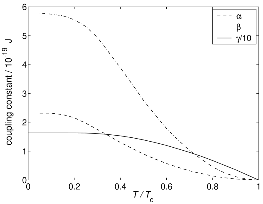
FIG. 3.: Temperature dependence of the tunneling model parameters $\alpha$, $\beta$ (68), and $\gamma$ (86) as calculated for a diffusive wall and total open area $A_{o}=A\kappa$ where, $A=3.8\cdot 10^{-8}$ m², $\kappa=14.7\cdot 10^{-4}$. The pressure is 0 bar, $W/D=0$, and $F_{i}^{a}=0$ for $i=1$, 3, etc.

The Josephson current (62) and energy (66) were obtained completely independently. It is essential to check that they are consistent with each other. One can easily see that the component $\mathop{\rm{Re}}d_{{\hat{{\bf{k}}}},{\hat{{\bf{k}}}}^{\prime}}$ satisfies

$$\mathop{\rm{Re}}d_{{\hat{{\bf{k}}}},{\hat{{\bf{k}}}}^{\prime}}(\epsilon_{m})=\frac{1}{2}\mathop{\rm Sgn}(\hat{k}_{z})\frac{\partial}{\partial\phi}\ln|s_{{\hat{{\bf{k}}}},{\hat{{\bf{k}}}}^{\prime}}(\epsilon_{m})|^{2},$$ (69)

and hence the macroscopic current formula (4) is exactly satisfied. As a further check of the energy (66) we can see that also the spin current formula (5) is satisfied. Using ${\bf{C}}^{\prime}_{L}\cdot{\bf{C}}_{R}=R^{L}_{\mu i}R^{R}_{\mu j}C^{\prime}_{i}C_{j}$ the energy (66) is seen to be a function of the products $R^{L}_{\mu i}R^{R}_{\mu j}$ and calculating the spin current from (5) is thus possible. Writing also $[{\bf{C}}^{\prime}_{L}\times{\bf{C}}_{R}]_{\gamma}=\epsilon_{\alpha\beta\gamma}R^{L}_{\alpha k}R^{R}_{\beta l}C^{\prime}_{k}C_{l}$ in the propagator component (58) and using the quasiclassical spin current expression (16) it can be checked that the result for $J_{\gamma}^{\rm spin}$ agrees with the one obtained from (5).

VII Textural interactions

As discussed in Sect. II, the Josephson effect in ³He depends on the rotation matrices $R_{\mu i}^{L,R}$ on the two sides of the weak link. These matrices are determined by the competition of a number of relatively weak bulk and surface interactions, which lift the degeneracy of the B phase order parameter (1). The equilibrium configuration is found by minimizing a hydrostatic energy functional. We shall present the hydrostatic theory to the extent needed here. For a recent review see Ref. [36].

A Interactions and coupling constants

The most important hydrostatic energy term arises from the dipole-dipole interaction between the nuclear magnetic moments,

$$F_{\rm{D}}=8g_{\rm{D}}\Delta^{2}\int{\mathrm{d}}^{3}r(\frac{1}{4}+\cos\theta)^{2},$$ (70)

where $\theta$ is the rotation angle of the spin-orbit rotation $R_{\mu i}(\hat{{\bf{n}}},\theta)$. The effect of $F_{\rm{D}}$ is to fix $\theta$ to the value $\theta_{0}\approx 104^{\circ}$ in the bulk liquid.

There is no conflict between $F_{\rm{D}}$ (70) and $F_{\rm{J}}$ (3). Even if $R_{\mu i}^{L,R}$ have their rotation angles fixed to $\theta_{0}$, $F_{\rm{J}}$ depends on their product $\psi_{ij}$ — also a rotation matrix — and it can attain all possible values if $\hat{{\bf{n}}}^{L}$ and $\hat{{\bf{n}}}^{R}$ are directed properly. Thus $\theta$ is not changed from $\theta_{0}$ by the Josephson coupling. The same applies to all surface energies below. We therefore assume $F_{\rm{D}}$ to be in its minimum everywhere and study only the position-dependence of $\hat{{\bf{n}}}({\bf{r}})$, which is known as the texture.

In the absence of a magnetic field the dominant interaction determining the texture near a wall is the surface-dipole interaction

$$F_{\rm{SD}}=\int_{S}{\mathrm{d}}^{2}r[b_{4}(\hat{{\bf{s}}}\cdot\hat{{\bf{n}}})^{4}-b_{2}(\hat{{\bf{s}}}\cdot\hat{{\bf{n}}})^{2}].$$ (71)

where $b_{2}$ and $b_{4}$ are positive coupling constants and $\hat{{\bf{s}}}$ is the surface normal. There are usually many walls with different orientations present and therefore there is a conflict between their orienting effects. This leads to gradient (bending) energy

$$F_{\rm{G}}=\int{\mathrm{d}}^{3}r\left[\lambda_{\rm{G1}}\frac{\partial R_{\alpha i}}{\partial r_{i}}\frac{\partial R_{\alpha j}}{\partial r_{j}}+\lambda_{\rm{G2}}\frac{\partial R_{\alpha j}}{\partial r_{i}}\frac{\partial R_{\alpha j}}{\partial r_{i}}\right],$$ (72)

which is related to spin currents in the bulk. The gradient energy also has a surface part

$$F_{\rm{SG}}=\lambda_{\rm{SG}}\int_{S}{\mathrm{d}}^{2}r\hat{s}_{j}R_{\alpha j}\frac{\partial R_{\alpha i}}{\partial r_{i}}.$$ (73)

In the presence of a magnetic field another surface interaction becomes important:

$$F_{\rm{SH}}=-d\int_{S}{\mathrm{d}}^{2}r({\bf{H}}\cdot\tensor{R}\cdot\hat{{\bf{s}}})^{2}.$$ (74)

There is also a bulk magnetic interaction

$$F_{\rm{DH}}=-a\int{\mathrm{d}}^{3}r(\hat{{\bf{n}}}\cdot{\bf{H}})^{2}.$$ (75)

The effect of stationary flow on the texture could be incorporated by the dipole-velocity interaction $F_{\rm{DV}}$, but the flow velocities in the experiment [5] are so small that $F_{\rm{DV}}$ is negligible.

The values of the many coefficients appearing above are discussed in Ref. [36] in some detail. However, most of them have only been evaluated in the GL region so far. As a byproduct of our calculation of the surface order parameter, we can now extend the calculations of $b_{2}$, $b_{4}$ and $\lambda_{\rm{SG}}$ to all temperatures.

The surface gradient parameter consists of two contributions $\lambda_{\rm{SG}}=\lambda_{\rm{SG}}^{a}+2\lambda_{\rm{G2}}$. The contribution $\lambda_{\rm{SG}}^{a}$ is equal to $J^{\rm{spin}}_{y,x}/L_{y}$, the current of $y$-directional spin projection in the $x$ direction per unit length in the $y$ direction ($L_{y}$), calculated for the order parameter $\mathchoice{{\hbox{\boldmath$\displaystyle\Delta$}}}{{\hbox{\boldmath$\textstyle\Delta$}}}{{\hbox{\boldmath$\scriptstyle\Delta$}}}{{\hbox{\boldmath$\scriptscriptstyle\Delta$}}}^{(0)}$. In terms of spin current density ${\bf j}^{\rm{spin}}_{\gamma}$ (16) it is given by

$$\lambda_{\rm{SG}}^{a}=\int_{0}^{\infty}{\mathrm{d}}zj^{\rm{spin}{(0)}}_{y,x}(z).$$ (76)

Figure 4 gives the temperature dependence of both terms of $\lambda_{\rm{SG}}$ for the cases of a specular and a diffusive wall.

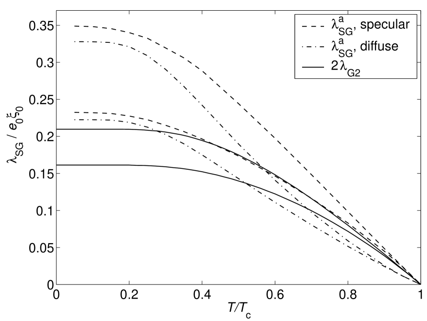
FIG. 4.: Gradient energy parameters $\lambda_{\rm{SG}}^{a}$ (dashed line: specular wall, dash-dotted line: diffusive wall) and $2\lambda_{\rm{G2}}$ (solid line) in the weak coupling approximation. The upper curves are for $F_{1}^{a}=0$ and the lower ones for $F_{1}^{a}=-1$. $F_{3}^{a}$ and higher order parameters are assumed zero. The unit is $e_{0}\xi_{0}$, where $e_{0}=\hbar v_{\mathrm{F}}N(0)k_{\mathrm{B}}T_{\rm c}$.

Close to $T_{\rm c}$ all of the parameters vanish linearly in $T-T_{\rm c}$. The slopes of $\lambda_{\rm{SG}}=\lambda_{\rm{SG}}^{a}+2\lambda_{\rm{G2}}$ agree with the GL results of Ref. [36] for vapor pressure; at low temperatures there is considerable deviation from the linear GL behavior. We have calculated the results for $F_{1}^{a}=0$ and $F_{1}^{a}=-1$, the true value at vapor pressure being probably somewhere in between. The change with $F_{1}^{a}$ is rather strong here, since $\lambda_{\rm{SG}}^{a}$ is directly related to the spin current.

The surface-dipole coupling constants $b_{2}$ and $b_{4}$ are given by [36]

$$b_{2} = \frac{5}{4}g_{\rm{D}}\int_{0}^{\infty}{\mathrm{d}}z(\Delta_{\perp}^{2}-6\Delta_{\perp}\Delta_{\parallel}+5\Delta_{\parallel}^{2})$$ (77)

$$b_{4} = \frac{25}{8}g_{\rm{D}}\int_{0}^{\infty}{\mathrm{d}}z(\Delta_{\parallel}-\Delta_{\perp})^{2}$$ (78)

at all temperatures. Figure 5 shows these two plotted as a function of $T/T_{\rm c}$.

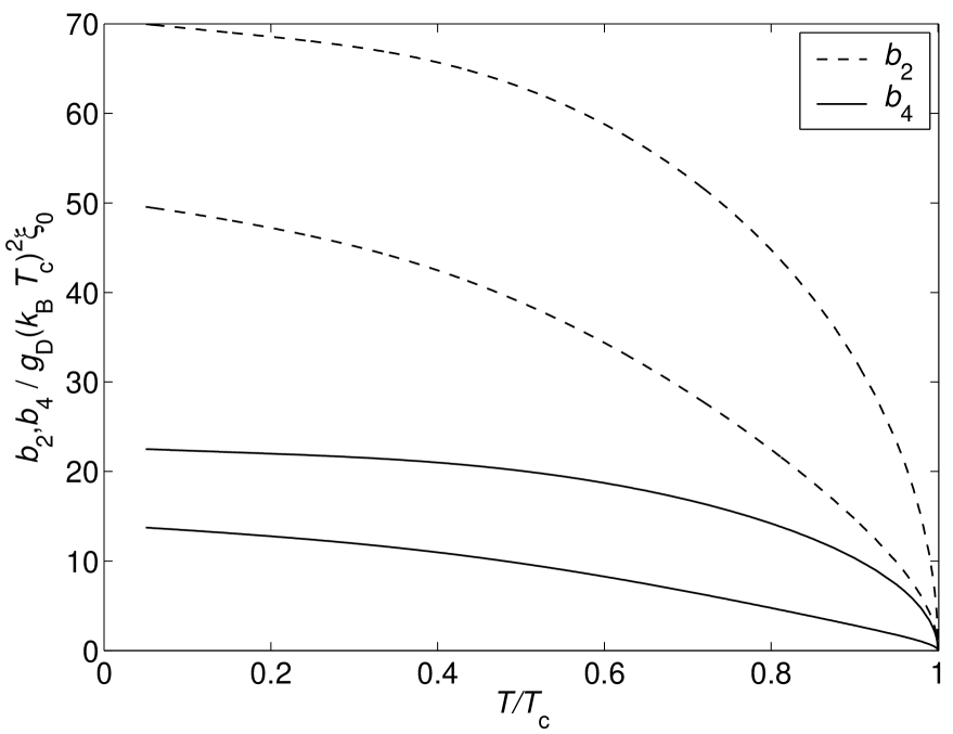
FIG. 5.: Surface dipole interaction parameters $b_{2}$ (dashed lines) and $b_{4}$ (solid lines) in the weak coupling approximation and with $F_{1}^{a}=0$. The lower of each pair is for a diffusive wall and the upper for a specular wall. The unit of $b_{2}$ and $b_{4}$ is $g_{\rm{D}}(k_{\mathrm{B}}T_{\rm c})^{2}\xi_{0}$.

Both of them go to zero proportional to $(1-T/T_{\rm c})^{1/2}$ near $T_{\rm c}$. In this region more accurate values can be obtained from the GL results [36], with which these coincide. Because $b_{2}>2b_{4}$, $F_{\rm{SD}}$ (71) favors $\hat{{\bf{n}}}$ perpendicular to the wall. The dependence of $b_{2}$ and $b_{4}$ on $F_{1}^{a}$ is much weaker than that of $\lambda_{\rm{SG}}$, since the effect of the spin current comes to play only through the order parameter. For $F_{1}^{a}=-1$ the values tend to be diminished by at most 5 percent from those shown in Fig. 5.

B Competing interactions and length scales

In dealing with the pinhole model, we are mostly interested in the behavior of the texture at different magnetic fields near a flat surface. In this case there are three relevant contributions to energy (per surface area $L^{2}$): (i) the surface-dipole energy, $F_{\rm{SD}}/L^{2}\approx b_{2}$, (ii) the surface-field energy, $F_{\rm{SH}}/L^{2}\approx dH^{2}$, and (iii) one related to the bending of the texture when there is a uniform perturbation at the wall (caused by $F_{\rm SH}$, for example) $(F_{\rm{G}}+F_{\rm{DH}})/L^{2}$ $\approx\sqrt{65\lambda_{\rm{G2}}aH^{2}/8}\propto H$. All of these have different field dependences, but their values turn out to coincide at $H\approx 1$ mT. It is seen that at fields $H\lesssim$ 1 mT the constant $F_{\rm SD}$ always dominates, and thus $\hat{{\bf{n}}}$ will be aligned perpendicular to the surface. For $H\gtrsim$ 1 mT the dominant surface interaction is $F_{\rm SH}$, and the local texture is determided by its minima.

The conclusion about the relative magnitudes of $F_{\rm SD}$ and $F_{\rm SH}$ is true also in general. However, to determine the texture at the surfaces in more complicated restricted geometries, the gradient and other bulk energies have to be minimized together with the surface energies. The surfaces can then be seen as perturbing the bulk texture which would otherwise be uniform. Associated with each hydrostatic interaction competing with the gradient energy, there is a characteristic length scale that describes the scale on which such local perturbations from uniformity will decay, or heal [37, 17]. The stronger the competing interaction, the shorter is the corresponding healing length. Comparing these healing lengths with the spatial scale $l\gg\xi_{0}$ of the container gives qualitative information on the form of the texture.

Most importantly, in the presence of a magnetic field $F_{\rm DH}$ and $F_{\rm G}$ define a length $\xi_{\rm H}=\sqrt{65\lambda_{\rm{G2}}/(8aH^{2})}\propto H^{-1}$ [36]. Comparison of $F_{\rm D}$ and $F_{\rm G}$ gives another one, the dipole length $\xi_{\rm D}=\sqrt{\lambda_{\rm{G2}}/g_{\rm{D}}\Delta^{2}}\approx 10~{}\mu$m $\gg\xi_{0}$, related to possible perturbations of the rotation angle $\theta$ from its equilibrium value $\theta_{0}$. As stated above, we assume there to be no interactions present which could force such perturbations, and therefore $\xi_{\rm D}$ plays no role. In any case, for most practical purposes $\xi_{\rm H},l\gg\xi_{\rm D}$, and such a perturbation would decay fast on the scale of $l$.

For very small magnetic fields $\xi_{\rm H}\gg l$ and $\xi_{\rm H}$ is thus also not a relevant length scale. The only important hydrostatic interactions in this case are the surface-dipole energy $F_{\rm SD}$ and the gradient energies $F_{\rm G}$ and $F_{\rm SG}$. Now the interesting question is simply whether the walls of the container are separated by long enough distances for $F_{\rm{SD}}$ to be essentially minimized, or small enough distances for no textural variation to occur at all — the minimum configuration of $F_{\rm{Gtot}}=F_{\rm{G}}+F_{\rm{SG}}$. An elementary estimation of the length scale $l$ at which there is a transition from one behavior to another gives $l\propto\lambda_{\rm{G2}}/(b_{2}-b_{4})$, where the constant of proportionality is of order unity. Since $b_{4}<b_{2}$, we can drop it and define a surface-dipole length $\xi_{\rm{SD}}\equiv\lambda_{\rm{G2}}/b_{2}$. Using the numerical values calculated above we get at zero pressure

$$\xi_{\rm{SD}}=\frac{\lambda_{\rm{G2}}}{b_{2}}\approx\left\{\begin{array}[]{ll}2.5~{}\rm{mm}&T\approx 0\\ 6.8(1-T/T_{\rm c})^{1/2}~{}\rm{mm}&T\approx T_{\rm c}.\end{array}\right.$$ (79)

VIII Isotextural Josephson effect

The Josephson energy (6) of a pinhole depends nontrivially on three parameters: the phase $\phi$ and two parameters describing $\psi_{ij}=R_{\mu i}^{L}R_{\mu j}^{R}$. In addition there is dependence on the surface scattering (diffusive vs. specular), on the temperature $T/T_{\rm c}$ and on $W/D$. Below we can present only some representative parts of this parameter space. In this section we plot isotextural current-phase relationships, where $\psi_{ij}$ is assumed constant in $J(\phi,\psi_{ij})$. The possible $\phi$ dependence of $\psi_{ij}$ is considered in Sec. IX.

The pinhole coupling has the maximal symmetry (6) independently of the shape of the hole as long as $W/D=0$. In terms of $\hat{{\bf{n}}}$ this means, for example, $F_{\rm J}(\phi,\hat{{\bf{n}}}^{L},\hat{{\bf{n}}}^{R})=F_{\rm J}(\phi,\hat{{\bf{n}}}^{R},\hat{{\bf{n}}}^{L})=F_{\rm J}(\phi,-\hat{{\bf{n}}}^{L},-\hat{{\bf{n}}}^{R})$, and similarly for the mass current. The mass current is given in units of $J_{0}=2m_{3}v_{\mathrm{F}}N(0)k_{\mathrm{B}}T_{\rm c}A_{o}$, where $A_{o}$ is the total open area of one or more pinholes. In most cases only the phase differences in the range $[0,\pi]$ are shown due to the symmetry $J(2\pi-\phi)=-J(\phi)$. All plots are made for $F_{1}^{a}=0$. Tests with $F_{1}^{a}=-1$ show no qualitative differences and at most a few percent quantitative difference in $J(\phi)$ even at the lowest temperatures.

A Spin-rotation axes perpendicular to wall

We first study the case where the spin-orbit rotation axes $\hat{{\bf{n}}}^{L,R}$ are perpendicular to the intervening thin wall. This situation is realistic if the external magnetic field is small enough ($H\lesssim 1$ mT) and if there are no other walls with different orientations nearby. Four different $\hat{{\bf{n}}}$ configurations are then possible, namely the combinations $\hat{{\bf{n}}}^{L,R}=\pm\hat{{\bf{z}}}$, where $\hat{{\bf{z}}}$ is normal to the wall. These give rise to two different current-phase relations corresponding to parallel ($\hat{{\bf{n}}}^{L}=\hat{{\bf{n}}}^{R}$) or antiparallel ($\hat{{\bf{n}}}^{L}=-\hat{{\bf{n}}}^{R}=\pm\hat{{\bf{z}}}$) situations. The parallel case is actually more general, because the $\hat{{\bf{n}}}$ vectors need not be perpendicular to the wall to still give the same $J(\phi)$. The current-phase relations are shown in Figs. 6-8 corresponding to three different surface models.

First we consider the case of constant order parameter. Here $\mathchoice{{\hbox{\boldmath$\displaystyle\Delta$}}}{{\hbox{\boldmath$\textstyle\Delta$}}}{{\hbox{\boldmath$\scriptstyle\Delta$}}}{{\hbox{\boldmath$\scriptscriptstyle\Delta$}}}({\hat{{\bf{k}}}},{\bf{r}})$ is not calculated self-consistently using any boundary condition, but instead is assumed to have its constant bulk form $\Delta{\hat{{\bf{k}}}}$ all the way to the wall (no pair breaking). This is the case discussed by Yip [10], and the current-phase relations shown in Fig. 6 are exactly the same as obtained by him.

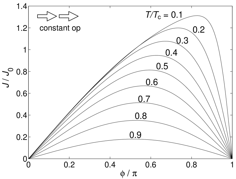
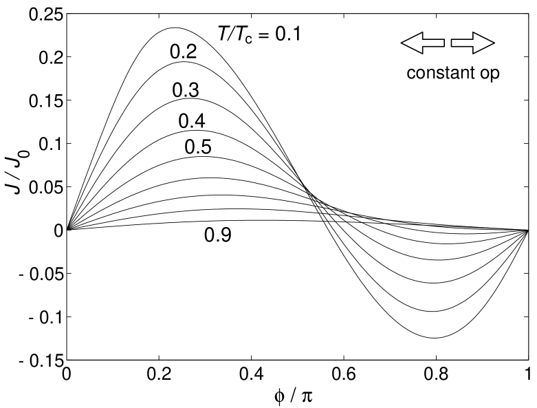
FIG. 6.: Isotextural current-phase relations for a pinhole in a wall with a constant order parameter on both sides. The top panel corresponds to $\hat{{\bf{n}}}^{L}=\hat{{\bf{n}}}^{R}$ and lower to $\hat{{\bf{n}}}^{L}=-\hat{{\bf{n}}}^{R}=\pm\hat{{\bf{z}}}$. $W/D=0$.

The parallel case is well known: the same result was first obtained by Kulik and Omel’yanchuk for microbridges in $s$-wave superconductors, and it was subsequently generalized to the case of ³He by Kurkijärvi [16]. The new feature found by Yip is seen in the antiparallel case: very close to $T_{\rm c}$ the $J(\phi)$ is sinusoidal, but at temperatures below about $0.5T_{\rm c}$ the $\pi$ state appears: a strong kink and a new zero of $J(\phi)$ appear around $\phi=\pi$.

The self-consistent surface models lead to considerable suppression of the order parameter at the wall. As a consequence, the $J(\phi)$’s are different for a specular surface and for a diffusive surface, shown in Figs. 7 and 8.

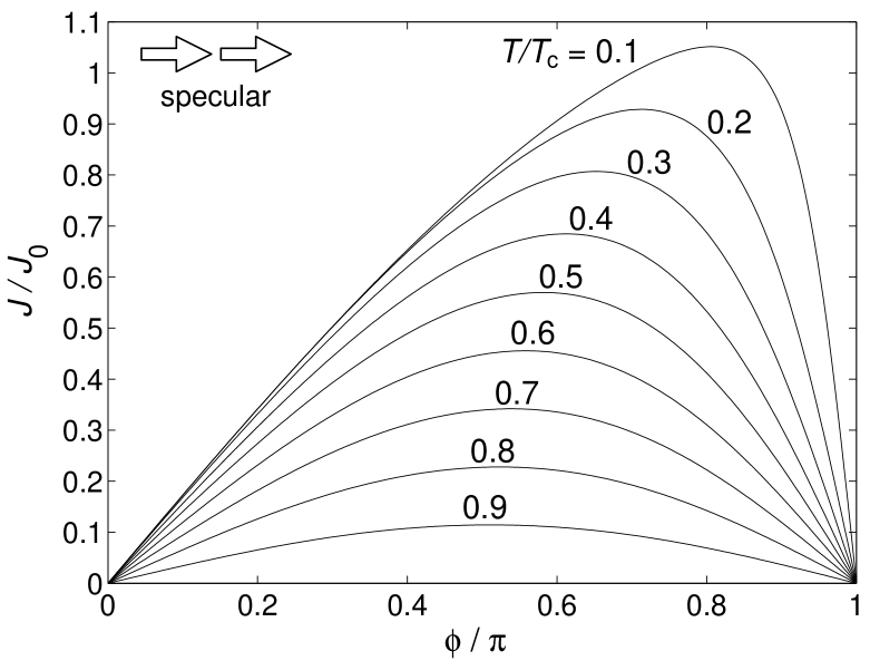
FIG. 7.: Isotextural current-phase relations for a pinhole in a specularly scattering wall. The top panel corresponds to $\hat{{\bf{n}}}^{L}=\hat{{\bf{n}}}^{R}$ and lower to $\hat{{\bf{n}}}^{L}=-\hat{{\bf{n}}}^{R}=\pm\hat{{\bf{z}}}$. $F_{1}^{a}=W/D=0$.

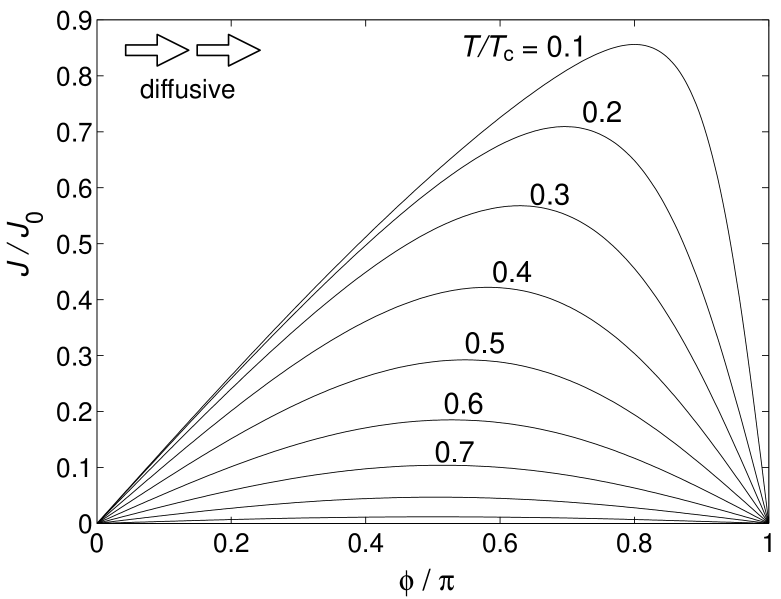
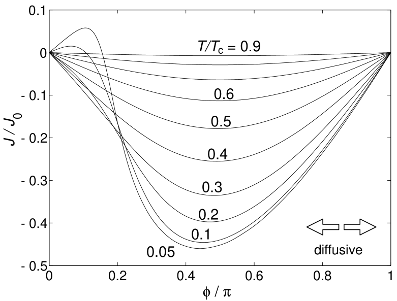
FIG. 8.: Isotextural current-phase relations for a pinhole in a diffusely scattering wall. The top panel corresponds to $\hat{{\bf{n}}}^{L}=\hat{{\bf{n}}}^{R}$ and lower to $\hat{{\bf{n}}}^{L}=-\hat{{\bf{n}}}^{R}=\pm\hat{{\bf{z}}}$. $F_{1}^{a}=W/D=0$.

Both surface models result in qualitatively similar $J(\phi)$’s. The parallel current-phase relations look similar as in Yip’s case, although their critical currents are slightly reduced. A clear difference is seen in the antiparallel cases: Firstly, the whole $J(\phi)$ appears to be shifted by $\pi$ so that on the phase interval $[0,\pi]$ the current is mostly negative. Secondly, the $J(\phi)$ remains sinusoidal down to very low temperatures. An additional kink begins to form only at around $0.2T_{\rm c}$. Now the kink is also shifted from $\phi=\pi$ to $\phi=0$. We continue to call it a $\pi$ state because it represents a local minimum of $F_{\rm J}(\phi)$ that is shifted from the from the global minimum of $F_{\rm J}(\phi)$ by the phase difference $\pi$.

Figure 9 shows the critical currents $J_{\rm c}$ and the possible additional extrema of $J(\phi)$ as a function of temperature.

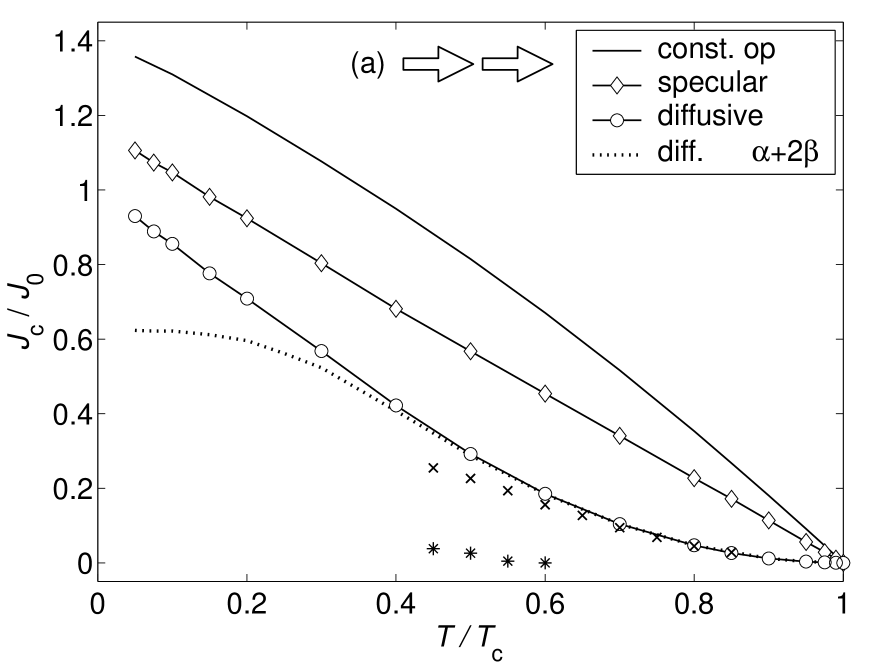
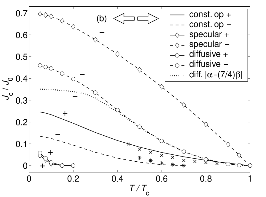
FIG. 9.: Critical currents as functions of the temperature. The lines (with and without markers) are theoretical pinhole results and separate points ($\times$, $*$) are experimental results [4] with $J_{0}=213$ ng/s (Sec. X). For theoretical results the upper and lower panels correspond to parallel and antiparallel $\hat{{\bf{n}}}$ vectors, respectively. For experimental results they correspond to the H and L states. The signs ($+$, $-$) denote the negative and positive extrema of $J(\phi)$ that appear in the case of antiparallel $\hat{{\bf{n}}}$’s. The experiment shows two extrema in both H and L cases, whose signs are unknown. The calculations are for $F_{1}^{a}=W/D=0$.

For parallel $\hat{{\bf{n}}}$ vectors such a plot has been published in Ref. [24], but there the pinhole results were erroneous. Close to $T_{\rm c}$, $J_{\rm c}(T)\propto 1-T/T_{\rm c}$ for a constant order parameter and a specular surface, and for a diffusive surface $J_{\rm c}(T)\propto(1-T/T_{\rm c})^{2}$, as expected from previous calculations [23]. The critical current for a constant order parameter is always the highest and for a diffusive wall the lowest. For antiparallel $\hat{{\bf{n}}}$ vectors the roles change: the constant order parameter case has the lowest $J_{\rm c}$, due to the strong cancellation between different quasiparticle directions, but the negative extremum around $\phi=\pi$ is nearly as pronounced as the positive one. It is clearly visible that the other extrema appear only at much lower temperatures for diffusive and specular surfaces.

The dotted lines correspond to the high-temperature approximations obtained from Eqs. (68) for a diffusive wall, i.e., $(2m_{3}/\hbar)(\alpha+2\beta)$ for parallel and $(2m_{3}/\hbar)[\alpha-(7/4)\beta]$ for antiparallel $\hat{{\bf{n}}}$’s. These lines follow the correct critical currents very well down to temperatures around $T=0.4T_{\rm c}$. The current-phase relations show some deviation from the sinusoidal form at temperatures above $0.4T_{\rm c}$ in specular and diffusive cases, but the deviation is much smaller than for a constant order parameter.

B Other orientations of spin rotation axes

In order to study other orientations of $\hat{{\bf{n}}}^{L,R}$ we consider first the case of relatively large magnetic fields, $H\gtrsim 1$ mT. The configurations, which minimize the surface magnetic interaction $F_{\rm{SH}}$ (74), depend on the angle $\theta_{H}$ between ${\bf{H}}$ and the wall normal $\hat{{\bf{s}}}=\hat{{\bf{z}}}$. Our results, obtained using the self-consistent order parameter for a specular and a diffusive wall, are qualitatively similar to Ref. [10], but differ in details. Figure 10 shows the four different $J(\phi)$’s which are possible at $\theta_{H}=0.45\pi$, corresponding to four different $\hat{{\bf{n}}}^{L,R}$ configurations $AA,AB,AC$ and $CD$, as defined in Ref. [10]. Also shown is the dependence of $J(\phi)$ on $\theta_{H}$, when the $\hat{{\bf{n}}}^{L,R}$ are in the $AB$ configuration.

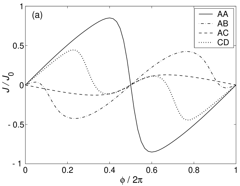
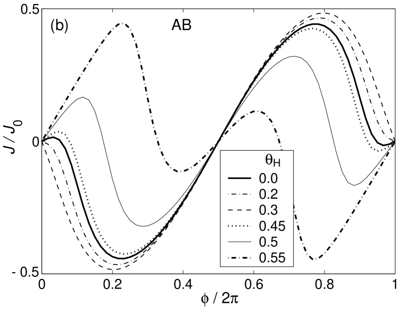
FIG. 10.: Examples of current-phase relations in high magnetic field. (a) The four possible $\hat{{\bf{n}}}$ configurations which result in different current-phase relations for magnetic field angle $\theta_{H}=0.45\pi$. The nomenclature follows the definitions of Ref. [10]. (b) The effect of varying $\theta_{H}$ in the $AB$ configuration. The values of $\theta_{H}$ are given in the legend. The curves are for a pinhole in a diffusive wall at $T=0.1T_{\rm c}$ with $F_{1}^{a}=W/D=0$.

For $\theta_{H}=0$ the $AB$ configuration gives the antiparallel case studied above. These should be compared with Figs. 4 and 5 of Ref. [10], where the same plots were given for the constant order parameter. It can be seen that $\pi$ states are not uncommon at low temperature $T\approx 0.1T_{\rm c}$.

For a systematic study it seems to be more economic to specify $\hat{{\bf{n}}}^{L,R}$ directly. Let us consider the case where the polar angle of $\hat{{\bf{n}}}^{L}$ is changed but $\hat{{\bf{n}}}^{R}$ is kept constant: $\hat{{\bf{n}}}^{L}\cdot\hat{{\bf{z}}}=\cos\eta^{L}$ and $\hat{{\bf{n}}}^{R}=\hat{{\bf{z}}}$. It can be seen in Fig. 11a that $J(\phi)$ differs essentially from the $\sin\phi$ shape around angles $\eta^{L}\approx 0.46\pi$.

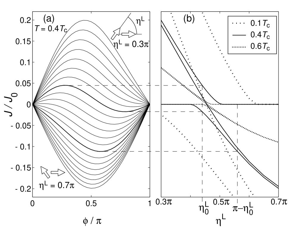
FIG. 11.: Change of isotextural current-phase relation (a) and extremal currents (b) as a function of $\eta^{L}=\arccos\hat{n}_{z}^{L}$ for $\hat{{\bf{n}}}^{R}=\hat{{\bf{z}}}$. In (a) the current-phase relations are shown at intervals $\Delta\eta^{L}=0.02\pi$ at temperature $0.4T_{\rm c}$. In (b) the extrema of $J(\phi)$ (top and bottom curves of each type) are compared with the tunneling model results (middle curves) at temperatures $T/T_{\rm c}=0.1$, $0.4$, and $0.6$. The angles $\eta^{L}_{0}$ and $\pi-\eta^{L}_{0}$ correspond to possible bistable states, as will be discussed in Sec. X A. The figure is calculated for diffuse scattering and $F_{1}^{a}=W/D=0$. In the specular case the relative deviation from the tunneling model is slightly larger ($\approx 20$ %).

The current is nearly proportional to $\sin(2\phi)$ at $\eta^{L}=0.46\pi$, and $\pi$ states are present in the range $\eta^{L}\approx 0.42\pi\ldots 0.50\pi$ at temperature $0.4T_{\rm c}$. The top and bottom solid lines in Fig. 11b show the extrema of $J(\phi)$ as a function of $\eta^{L}$. The middle solid line shows the prediction of the tunneling model. The tunneling model (7) has always sinusoidal isotextural $J(\phi)=J_{\rm c}\sin\phi$, where $J_{\rm c}=(2m_{3}/\hbar)E_{\rm c}$ and $E_{\rm c}=\alpha R_{\mu z}^{L}R_{\mu z}^{R}+\beta(R_{\mu x}^{L}R_{\mu x}^{R}+R_{\mu y}^{L}R_{\mu y}^{R})$. Therefore, it has only a single extremum value $J_{\rm c}$ (in the range $0<\phi<\pi$). Fig. 11b shows that the $\pi$ states (where two extrema appear) take place around the configuration where $J_{\rm c}$ changes sign by going through zero.

Fig. 11b shows the extrema at three different temperatures. At high temperatures the range where $\pi$ states occur is very narrow. Also, in configurations showing a $\pi$ state, both the negative and positive extrema of $J(\phi)$ are much reduced relative to the maximal critical currents shown in Fig. 9a. Outside of the range where $E_{\rm c}\approx 0$, $J(\phi)$ is nearly sinusoidal and the critical current is well predicted by the tunneling model. With decreasing temperature the range of the configurations showing a $\pi$ state widens and the extrema get larger. These results are not restricted to the case where $\hat{{\bf{n}}}^{R}=\hat{{\bf{z}}}$ but are valid for general configurations of $\hat{{\bf{n}}}^{L,R}$. This can be seen as a manifestation of a general difference between tunneling junctions and weak links, as discussed in Ref. [38]. In situations where a tunneling supercurrent is prohibited by symmetry, there can still be a small supercurrent flowing in a corresponding weak link, although with some restrictions on the form of $J(\phi)$.

C Nonzero $W/D$

Let us consider quasiparticle scattering inside a pinhole caused by a finite aspect ratio $W/D$. In a $p$-wave superfluid this can lead to a current-phase relationship which is more complicated than some average of the ones obtained using tunneling model and direct transmission. Consider a deflected trajectory (Fig. 2) which is transmitted but the momentum direction is nearly reversed. Assume $\hat{{\bf{n}}}^{L}=\hat{{\bf{n}}}^{R}$. If the phase difference $\phi$ is zero, the quasiparticles of ³He see effectively a change in the sign of the order parameter $\mathchoice{{\hbox{\boldmath$\displaystyle\Delta$}}}{{\hbox{\boldmath$\textstyle\Delta$}}}{{\hbox{\boldmath$\scriptstyle\Delta$}}}{{\hbox{\boldmath$\scriptscriptstyle\Delta$}}}({\hat{{\bf{k}}}})$ along such a trajectory. However, if $\phi$ is near $\pi$, such quasiparticles see effectively a constant order parameter. This means that the scattering reduces the energy at $\phi=\pi$ relative to the energy at $\phi=0$. This could work as a mechanism for the formation of $\pi$ states even when the spin-rotation axes on the two sides are equal. This mechanism is closely related to the $\pi$ state mechanism of Ref. [10] and the effects discussed in Ref. [39] for $sd$ contacts.

The effect of the scattering on the current-phase relation is shown in Fig. 12.

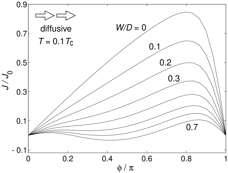
FIG. 12.: Current-phase relations for diffusive scattering in the aperture for $T/T_{\rm c}=0.1$, $F_{1}^{a}=0$ and $W/D=0.0\ldots 0.7$ in order of decreasing critical current. The $\hat{{\bf{n}}}$ vectors on are parallel on the two sides of the junction.

The main change is the decrease of the critical current. Contrary to our expectation of forming a $\pi$ state, a dip develops at $\phi\approx\pi/4$ with increasing $W/D$. However, this happens only in the region of $W/D$ where the distribution (36) has probably ceased to be valid. For small $W/D$ the only effect is to reduce the critical current, and the relative initial decrease does not seem to depend essentially on the temperature. The results for specular scattering are very similar.

IX Anisotextural Josephson effect

In the previous section we assumed that the $\hat{{\bf{n}}}$ texture remains constant when the phase difference $\phi$ is changed. In this section we study the anisotextural Josephson effect where the texture is allowed to change as a function of $\phi$ [11]. We demonstrate the anisotextural effect using a simple model. The possible existence of either isotextural or anisotextural Josephson effects in the Berkeley experiment [5] is discussed in Sec. X.

A Phenomenological model

We consider a planar wall separating two half-spaces of ³He-B. In the absence of perturbations, the surface interaction (71) fixes a constant texture on both sides. The orientations on left and right hand sides are denoted by $\hat{{\bf{n}}}^{L}_{\infty}$ and $\hat{{\bf{n}}}^{R}_{\infty}$, respectively. They both are either parallel or antiparallel to the normal $\hat{{\bf{z}}}$ of the wall: $\hat{{\bf{n}}}^{L}_{\infty}=\pm\hat{{\bf{z}}}$ and $\hat{{\bf{n}}}^{R}_{\infty}=\pm\hat{{\bf{z}}}$. Let us now place a weak link in the wall. The Josephson coupling energy $F_{\rm J}$ (3) may now favor a different orientation $\hat{{\bf{n}}}^{L,R}\not=\pm\hat{{\bf{z}}}$ at the junction. Such a change is opposed by a “rigidity energy”, which consists of gradient energy and possibly other textural energies (70)-(75). We model the rigidity energy by a quadratic form

$$F_{\rm{rig}}=\gamma^{L}(\eta^{L}-\eta^{L}_{\infty})^{2}+\gamma^{R}(\eta^{R}-\eta^{R}_{\infty})^{2}.$$ (80)

Here $\eta^{L,R}$ and $\eta^{L,R}_{\infty}$ are the polar angles of $\hat{{\bf{n}}}^{L,R}$ and $\hat{{\bf{n}}}^{L,R}_{\infty}$, respectively. In the case of symmetric left and right sides, the stiffness (or rigidity) parameters $\gamma^{L,R}$ are equal ($\gamma^{L}=\gamma^{R}=\gamma$), but the more general form will be useful later.

The texture is now found by minimizing the free energy

$$F=F_{\rm J}(\phi,\hat{\bf n}^{L},\hat{\bf n}^{R})+F_{\rm{rig}}(\hat{\bf n}^{L},\hat{\bf n}^{R},\hat{{\bf{n}}}^{L}_{\infty},\hat{{\bf{n}}}^{R}_{\infty})$$ (81)

with respect to $\hat{{\bf{n}}}^{L}$ and $\hat{{\bf{n}}}^{R}$. If the stiffness parameters $\gamma^{L,R}$ are sufficiently small, this will lead to a $\phi$ dependent texture. This is easiest to see using the tunneling model (7) for $F_{\rm J}$. If $\cos\phi>0$, the minimum $F_{\rm J}=-(\alpha+2\beta)\cos\phi$ is achieved by $\hat{\bf n}^{L}=\hat{\bf n}^{R}$. In the opposite case $\cos\phi<0$ the minimum $F_{\rm J}=-(\alpha-2\beta)\cos\phi$ (assuming $\alpha<\beta$) is achieved by $\hat{\bf n}^{L,R}=(\mp\hat{\bf x}+\hat{\bf y}\mp\sqrt{3}\hat{\bf z})/\sqrt{5}$, for example. Neglecting the rigidity (80), this leads to a $\pi$ state with a piecewise sinusoidal current-phase relation

$$J(\phi)=\cases{(2m_{3}/\hbar)(\alpha+2\beta)\sin\phi&for $\cos\phi>0$\cr(2m_{3}/\hbar)(\alpha-2\beta)\sin\phi&for $\cos\phi<0$\cr}.$$ (82)

This ideal current-phase relation is smoothed by finite $\gamma^{L,R}$. With increasing stiffness, the texture changes less as a function of $\phi$, and for $\gamma^{L,R}\gg\alpha$, $\beta$ the current-phase relation reduces to the isotextural one.

B Model parameters

Instead of using the tunneling model, we now assume the weak link to consist of an array of pinholes. The phase $\phi$ and $\hat{{\bf{n}}}^{L,R}$ are assumed to be constants over the array. Consequently, we can use the single-pinhole results for current (62) and coupling energy (66) simply by replacing the open area $A_{o}$ by the total area of the array $A$ times $\kappa$, the fraction of area occupied by the holes.

We start to estimate $\gamma$ including first only the gradient energy:

$$F_{\rm{rig}} = \frac{5}{8}\lambda_{\rm{G2}}\int{\mathrm{d}}^{3}r\Big{[}16(\partial_{i}\hat{n}_{j})(\partial_{i}\hat{n}_{j})$$ (84)

$$-(\sqrt{3}\nabla\cdot\hat{{\bf{n}}}+\sqrt{5}\hat{{\bf{n}}}\cdot\nabla\times\hat{{\bf{n}}})^{2}\Big{]}.$$

This can be obtained from the sum of gradient energies (73) and (72) assuming $\lambda_{\rm{SG}}=4\lambda_{\rm{G2}}$ and $\lambda_{\rm{G1}}=2\lambda_{\rm{G2}}$; see also Ref. [37]. We shall assume that $\hat{{\bf{n}}}$ varies only in one plane, the $xz$ plane, for example. This allows one to describe $\hat{{\bf{n}}}$ by its polar angle $\eta$ alone: $\hat{{\bf{n}}}=\cos\eta\hat{{\bf{z}}}+\sin\eta\hat{{\bf{x}}}$. In addition, we can assume $\eta$ to depend only on the radial direction $r$ from the center of the aperture array. With these assumptions the energy (84) on one side simplifies to

$$F_{\rm{rig}}^{L}=\frac{50\pi}{3}\lambda_{\rm{G2}}\int{\mathrm{d}}rr^{2}(\partial_{r}\eta)^{2}.$$ (85)

This is minimized by a function of the form $\eta(r)=A/r+C$, but to avoid a divergence at $r=0$, we have to cut off the integration at some $r$, for example at the radius of the array $R=\sqrt{A/\pi}$. As a result one finds the form (80) with the stiffness parameter

$$\gamma=\frac{50\pi}{3}\lambda_{\rm{G2}}R.$$ (86)

The rigidity has also a contribution form the surface-dipole interaction (71). It can be shown that this correction to $\gamma$ is proportional to $R/\xi_{\rm SD}$ when the radius of the array $R$ is small compared to $\xi_{\rm SD}$ (79). We assume this to be the case, and therefore neglect the small correction.

In order to get numerical values for $\gamma$ (86) we use the Berkeley array, where $R\approx 0.11$ mm [5]. The temperature dependence is given by $\lambda_{\rm{G2}}$, shown in Fig. 4. The resulting $\gamma(T)$ is plotted in Fig. 3. We use this value as a standard, to which the parameters $\gamma^{L,R}$ used in our calculations are referred to. Note that the reference value $\gamma$ of the rigidity energy is larger by one order of magnitude than $\alpha$ and $\beta$, which give the magnitude of the Josephson coupling energy (Fig. 3).

In order to calculate the current, the free energy (81) should be minimized with respect to three angles parametrizing $\hat{{\bf{n}}}^{L,R}$: $\eta^{L},\eta^{R}$ and the relative azimuthal angle $\chi$. The results of such a minimization for $\gamma^{L}=\gamma^{R}=0.1\gamma$ are shown in Figure 13.

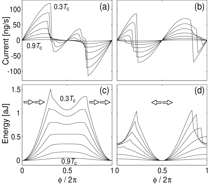
FIG. 13.: Anisotextural current-phase $J(\phi)$ and energy-phase $F(\phi)$ relations for bistable states $\eta^{L}_{\infty}=0$ (a,c) and $\eta^{L}_{\infty}=\pi$ (b,d). The curves correspond to different temperatures at intervals of $0.1T_{\rm c}$. The arrows indicate the $\hat{{\bf{n}}}$ orientations of in the zero branch, where $\hat{{\bf{n}}}^{L}=\hat{{\bf{n}}}^{L}_{\infty}$ and $\hat{{\bf{n}}}^{R}=\hat{{\bf{n}}}^{R}_{\infty}$. The rigidities on both sides are equal, $\gamma^{L}=\gamma^{R}=0.1\gamma$ and $\eta^{R}_{\infty}=0$. The weak link parameters and $\gamma$ (Fig. 3) are evaluated for the Berkeley array (Sec. X). The wall is assumed diffusive, $F_{1}^{a}=W/D=0$.

In creating these curves, we proceeded from left to right, using the minimum angles ($\eta^{L},\eta^{R},\chi$) of each $\phi$ step as the initial guess for the next step. The panels on the left are for the parallel case ($\eta^{L}_{\infty}=\eta^{R}_{\infty}=0$). For $\phi$ from $0$ to approximately $\pi/2$, the vectors $\hat{{\bf{n}}}^{L,R}$ remain exactly perpendicular to the wall. At low temperatures, a discontinuous jump to another branch of $J(\phi)$ occurs at around $\phi=\pi/2$, where $\hat{{\bf{n}}}^{L,R}$ are tilted form their original perpendicular positions. With increasing $\phi$ there is a jump back from this $\pi$ branch so that for $\phi>3\pi/2$ the minimum solution again corresponds to perpendicular $\hat{{\bf{n}}}$’s. The panels on the right are for the antiparallel case ($\eta^{L}_{\infty}=\pi$, $\eta^{R}_{\infty}=0$). Here the $\pi$ branch, where $\hat{{\bf{n}}}$’s are tilted, occurs not at $\phi\approx\pi$ but at $\phi\approx 0$. The fact that the curves are not (anti)symmetric with respect to $\phi=\pi$ indicates that the jumps between different branches are hysteretic.

We have studied the effect of increasing $\gamma^{L}=\gamma^{R}$ from the value $0.1\gamma$. We find that the $\pi$ state first disappears in the antiparallel case and then also in the parallel case. For example, the $\pi$ state in the parallel case [defined as positive $J^{\prime}(\pi)$] disappears when $\gamma^{L,R}\approx 0.2\gamma$ at $T=0.4T_{\rm c}$. The anisotextural effect on the current-phase relation still continues up to $\gamma^{L,R}\approx 0.7\gamma$. Since the coupling (66) scales with $A_{o}=A\kappa=\pi R^{2}\kappa$ and stiffness (86) with $R$, we get the following necessary condition for the appearance of $\pi$ states in the parallel case at temperatures $T\gtrsim 0.4T_{\rm c}$

$$R\kappa>0.5\ \mu\rm{m}.$$ (87)

Thus, the larger the radius $R$ of the array and the higher the ratio of the open area $\kappa$, the better are the chances of realizing the anisotextural $\pi$ state. At higher temperatures it will be more difficult, due to the relative strength

It is interesting to compare the condition (87) with the Ginzburg-Landau calculation in a single large hole [11]. There $\pi$ states could be seen for hole radii $R>5.5\xi_{\rm{GL}}$. Setting $\kappa=1$ and extrapolating $\xi_{\rm{GL}}(0.4T_{\rm c})=8.8$ nm [36], we have the condition $R\kappa>0.48\ \mu$m in surprising agreement with the pinhole result above.

C Asymmetric case

We go slightly beyond the simple model of an infinite planar wall introduced in Sec. IX A. Firstly, we allow the asymptotic directions $\hat{{\bf{n}}}^{L,R}_{\infty}$ to be arbitrary. Secondly, the stiffness coefficients $\gamma^{L,R}$ can be different. In Fig. 14 we have studied different values of $\eta^{L}_{\infty}$ while $\eta^{R}_{\infty}=0$, $\gamma^{L}=0.3\gamma$, and $\gamma^{R}=\gamma$.

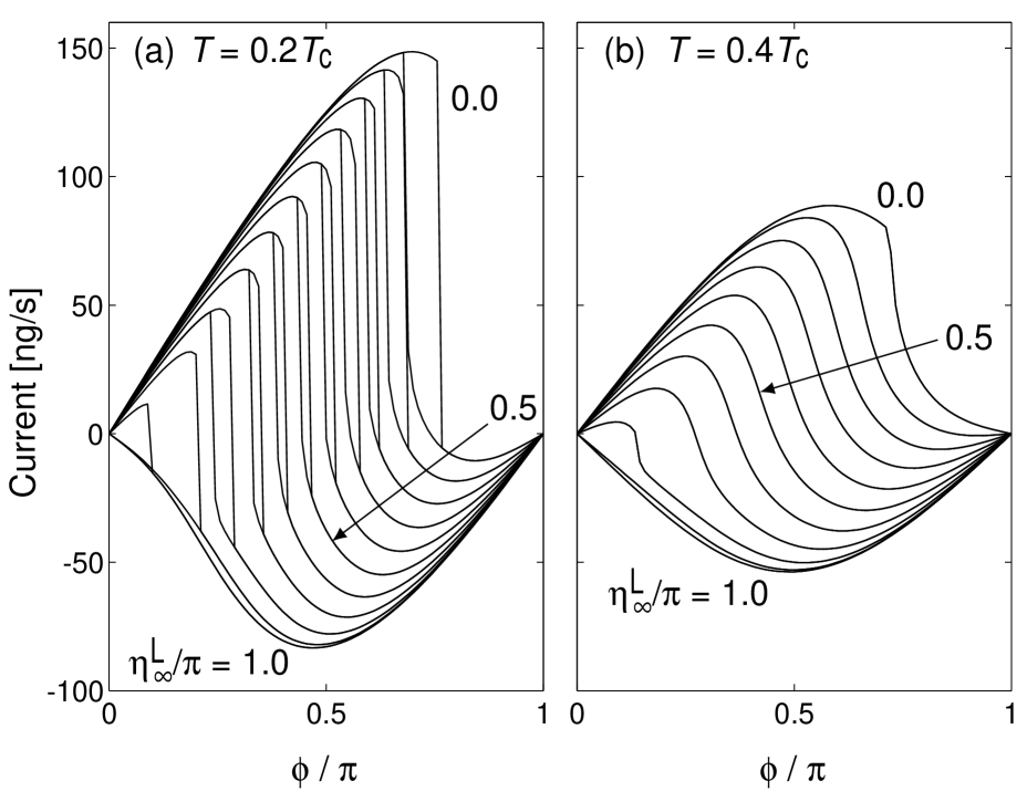
FIG. 14.: Anisotextural $J(\phi)$ for different asymptotic angles $\eta^{L}_{\infty}$ at temperatures $0.2T_{\rm c}$ (a) and $0.4T_{\rm c}$ (b). The other parameters are $\eta^{R}_{\infty}=0$, $\gamma^{L}=0.3\gamma$, and $\gamma^{R}=\gamma$. The different curves correspond to $\eta^{L}_{\infty}$ at intervals of $0.1\pi$. Other parameters are the same as in Fig. 13.

Here the extreme curves represent parallel and antiparallel $\hat{{\bf{n}}}^{L,R}_{\infty}$. It can be seen that neither of them have a $\pi$ state at $0.4T_{\rm c}$ and only the parallel case has one at $0.2T_{\rm c}$. However, at intermediate $\eta^{L}_{\infty}$ the $\pi$ states still persist in a wide range of $\eta^{L}_{\infty}$. The current-phase relationships are not hysteretic at high temperature, but hysteresis develops at lower temperatures. Figure 14 should be compared with the corresponding isotextural Fig. 11. In the isotextural case the $\pi$ states occur only in limited range, and there is no hysteresis.

The states with $\eta^{L}_{\infty}=\pi/2\pm{\rm constant}$ are expected to be degenerate in the absence of the Josephson coupling ($\eta^{R}_{\infty}=0$). The currents and energies for one pair of such bistable states are shown in Fig. 15.

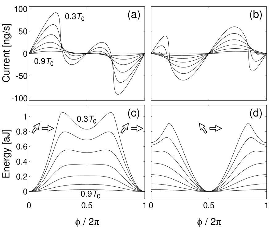
FIG. 15.: Anisotextural $J(\phi)$ and $F(\phi)$ for bistable states $\eta^{L}_{\infty}=0.3\pi$ (a,c) and $\eta^{L}_{\infty}=0.7\pi$ (b,d). The textures have different rigidities $\gamma^{L}=0.3\gamma$, $\gamma^{R}=\gamma$ and $\eta^{R}_{\infty}=0$. Other parameters are the same as in Fig. 13.

The important difference to Fig. 13 is that the curves are smooth and there is no hysteresis. In the case of parallel and antiparallel $\hat{{\bf{n}}}_{\infty}$’s the symmetry is spontaneously broken in the $\pi$ branch, whereas the tilted $\hat{{\bf{n}}}_{\infty}^{L}$ already breaks the symmetry, and thus the $\pi$ state can develop continuously.

D Discussion

The results of Figs. 13-15 contain both the isotextural and anisotextural mechanisms of $\pi$ states. However, practically the same results can be obtained all the way down to $T=0.4T_{\rm c}$ by using the tunneling model $F_{\rm J}$ (7), which excludes the isotextural $\pi$ state. As discussed above, the tunneling model fails at high temperatures only if the Josephson energy is close to zero. The minimization procedure seems to avoid such a situation, and thus the tunneling model gives a good description of the anisotextural pinhole array at temperatures above $T\approx 0.4T_{\rm c}$.

Here we comment our earlier calculations of the anisotextural Josephson effect in Ref. [11]. Firstly, there the tunneling model was used instead of the general pinhole result. Secondly, the scattering within the hole was partially taken into account by reducing the transmission by factor $p(\vartheta)$ (35), but the deflected trajectories were completely neglected. Thirdly, the coupling parameters $\alpha$ and $\beta$ were scaled by different factors, which is not possible when using the general pinhole result. Taken together, these explain why Fig. 13 is different from Fig. 2 in Ref. [11].

To be accurate, we should add to the preceding calculation the effect of the flow in the macroscopic region far away from the weak link. Above the phase difference $\phi$ is defined between the macroscopic-mesoscopic borders of the two sides (Fig. 1). The “true” phase difference between the infinities can be obtained by adding $(2m_{3}/\hbar)J/(\pi R\rho_{s})$ to $\phi$, where the correction assumes a radial flow outside of the radius $R$. Correspondingly the total energy gets an additional contribution $J^{2}/(2\pi R\rho_{s})$. These rescalings do not affect the results qualitatively.

The anisotextural model, as described above, assumes a vanishingly small external magnetic field. Qualitatively, it is easy to see what the effect of a strong magnetic field would be. In a field $H\gg 1$ mT, the strongest interaction affecting the texture is the surface-magnetic term $F_{\rm SH}$ (74). If the coupling energy scale is much smaller than this, then the texture will be fixed to some minimum of $F_{\rm SH}$ and will not depend on the phase difference. A strong magnetic field therefore suppresses any anisotextural $\pi$ state and only the isotextural mechanism remains.

In order to estimate the critical field, we equate the change in magnetic surface energy $\Delta F_{\rm SH}\approx dA{H}^{2}$ at the junction with the gain of energy $\Delta E$ between the $\pi$ state and “0 branch” at $\phi=\pi$. Thus $H_{\rm c}\approx\sqrt{\Delta E/(dA)}$. For the Berkeley array [5] $\Delta E$ can be estimated from the energy-phase graphs of Figs. 13 and 15 or from the experiments. At $T\approx 0.45T_{\rm c}$ the values are on the order of $\Delta E\approx 0.1\ldots 0.5$ aJ, which yields the order of magnitude $H_{\rm c}\approx 10\ldots 50$ mT.

X Analysis of the Berkeley experiment

We now turn to an analysis of the Berkeley experiment [5]. There the weak link consists of a square array of $65\times 65$ holes. They were etched in a $50$ nm thick silicon chip with a hole spacing of 3 $\mu$m, making the area of the array 195 $\mu$m $\times$ 195 $\mu$m. The holes were nominally squares $100$ nm $\times$ $100$ nm. However, flow resistance measurements in the normal state seem to indicate a somewhat larger apertures $115$ nm $\times$ $115$ nm [40], and these larger values are used in all numerical estimates in this paper. A sketch of the experimental cell is shown in Fig. 16.

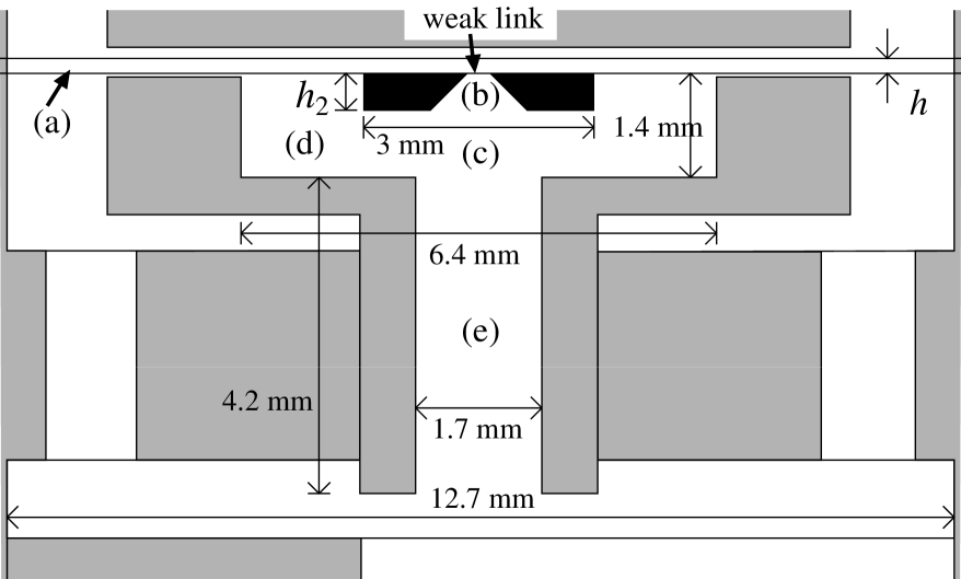
FIG. 16.: Part of the experimental cell in Ref. [5]. Most of the structure has rotation symmetry around the vertical axis. The “pillbox” (a) between two flexible membranes (diameter 1.27 cm, distance $h=0.14$ mm) forms a volume that is connected to the rest of ³He volume only through the weak link. The weak link is made in a silicon chip attached to the lower membrane. The chip is $h_{2}=0.5$ mm thick and has a square window opening from 250 $\mu$m $\times$ 250 $\mu$m to some 0.95 mm $\times$ 0.95 mm at the lower chip surface. The figure is based on a drawing supplied by S. Pereverzev.

The scattering properties of ³He quasiparticles from the silicon chip are not known, but most surfaces are generally believed to be diffusively scattering. The magnetic field is believed to be small, $H\ll 1$ mT, and the pressure is 0 bar. We further assume the system to be in thermal equilibrium.

The central experimental findings are the bistability and the existence of $\pi$ states [5]. Bistability means that the system can randomly choose between two alternative states, characterized by high (H) and low (L) critical currents. Both of these states show $\pi$ states. The measured extremal currents are plotted in Fig. 9.

There are two major difficulties in applying the theory presented in this paper to the Berkeley experiment. Firstly, since $\xi_{0}=77$ nm, the holes are too large to be pinholes. Also, the holes are too small for the Ginzburg-Landau calculations to be reliable [14, 11]. We use the pinhole model because more accurate calculations would be much more demanding. Moreover, due to the approximate nature of our pinhole calculations for finite aspect ratio $W/D$, we will only use the pinhole theory in the limit $W/D=0$, although experimentally $W/D\approx 0.4$. Another reason for using $W/D=0$ is that the measured critical currents are clearly larger than calculated for pinholes with $W/D=0.4$ (Sec. VIII C). The second major difficulty is that the cell is complicated, and its dimensions are on the same order of magnitude as $\xi_{\rm{SD}}$ (79). Instead of a proper calculation of the texture, we will make some simple estimates and introduce one adjustable parameter.

A Isotextural Josephson effect

Here we consider the case where the Josephson coupling can be considered as a weak perturbation, which does not affect the texture on either side of the weak link. For small magnetic field, the dominant orienting effect on $\hat{{\bf{n}}}$ comes from the surface-dipole energy (71). In region (a) of Fig. 16 this clearly favors the uniform texture $\hat{{\bf{n}}}=\pm\hat{\bf z}$, where $z$ is along the axis of the cell. The situation is more complicated on the other side of the junction. The axial orientation is preferred in the wide cylindrical region (d). The narrow cylindrical region (e) favors $\hat{{\bf{n}}}\perp\hat{{\bf{z}}}$. The tendencies from regions (d) and (e) compete in region (c) below the chip, and affect the texture in the window region (b). Let us assume that the minimization of textural energies (70)-(75) favors at the junction a particular orientation of $\hat{{\bf{n}}}^{L}=\hat{{\bf{n}}}^{L}_{0}$ with polar angle $\eta^{L}_{0}$. Then there must be a degenerate textural state with $\hat{{\bf{n}}}^{L}=-\hat{{\bf{n}}}^{L}_{0}$, which corresponds to the polar angle $\eta^{L}=\pi-\eta^{L}_{0}$. There can be additional degeneracy with respect to the azimuthal angle.

When we add the pinhole Josephson coupling, the degenerate states above give rise to precisely two different current-phase relationships if $\eta^{L}_{0}\not=\pi/2$. These two are obtained by studying configurations with $\eta^{L}=\eta^{L}_{0}$ and $\eta^{L}=\pi-\eta^{L}_{0}$ with a fixed $\hat{{\bf{n}}}^{R}=\hat{\bf z}$. Configurations of this kind were studied above in Fig. 11. They can in principle explain both the bistability and the existence of $\pi$ states. Quantitative comparison with experiment gives, however, very poor agreement. The problem is to fit the four experimental points in Fig. 9 at any temperature with the four extrema in Fig. 11b at angles $\eta^{L}_{0}$ and $\pi-\eta^{L}_{0}$ using $\eta^{L}_{0}$ as a fitting parameter. One such construction at $T=0.4T_{\rm c}$ is shown by vertical lines in Fig. 11b. In that case, one finds the L state with a $\pi$ state, but then no $\pi$ state appears in the H state, and all currents are more than by a factor of 2 too small. Alternatively, if one tries to fit the critical current in the H state, one has to approach the parallel and antiparallel states, where no $\pi$ states appear at this temperature (Figs. 7-9).

B Anisotextural Josephson effect

For the anisotextural Josephson effect we have to calculate the rigidity energy (80). The region (a) is much thinner than $\xi_{\rm SD}$ and therefore we have to consider a two-dimensional texture instead of the 3D in Sec. IX B. In the present case the surface interaction is important. We find that $\gamma^{R}$ is proportional to $\lambda_{\rm G2}h/\ln(\sqrt{h\xi_{\rm SD}}/R)$ instead of $\lambda_{\rm G2}R$ (86), but these two happen to be of the same order of magnitude. Thus the texture in region (a) is rather stiff, and we assume $\gamma^{R}\approx\gamma$. This makes the texture essentially fixed.

In order to analyze the other side (L), we first consider a conical region between two radii, $R_{1}$ and $R_{2}$. Otherwise, we use the same approximations as for the half space in Sec. IX B. We get the rigidity energy

$$F_{\rm rig}^{(1-2)}=\frac{50\pi}{3}\lambda_{\rm{G2}}(1-\cos\theta)\frac{R_{1}R_{2}}{R_{2}-R_{1}}[\eta(R_{1})-\eta(R_{2})]^{2},$$ (88)

where $\theta$ is the opening angle of the cone. This reduces to the previous result (86) in the limit $\theta=\pi/2$ and $R_{2}=\infty$. We now consider the regions (b) and (c) as three consecutive conical regions. The middle one corresponds to the conical region of the chip with $\theta=\theta_{w}\approx 38^{\circ}$, the two others have $\theta=\pi/2$. We neglect the effect of regions (d) and (e) and assume that region (c) extends to infinity. For the combined stiffness of these regions we get the estimate

$$\gamma^{L}\approx\frac{50\pi}{3}\lambda_{\rm{G2}}\left[\frac{1}{R}+\frac{\cos\theta_{w}}{1-\cos\theta_{w}}\left(\frac{1}{R_{1}}-\frac{1}{R_{2}}\right)\right]^{-1},$$ (89)

where $R_{1}$ and $R_{2}$ are the radii of the inner and outer edges of the conical region measured from the weak link. Substituting the numerical values we find $\gamma^{L}\approx 0.31\gamma$, where $\gamma$ is the half-space value (86). Thus this side is considerably softer than the other.

The calculations for the present parameters have already been done in Sec. IX C. The results are presented in Fig. 14 for different angles $\eta^{L}_{\infty}$. A representative pair of bistable states is presented in Fig. 15. The calculated current-phase relations are very similar to those found experimentally [5]. The $\pi$ states are present in both bistable states. The critical current in the H state (identified with $\eta^{L}_{\infty}\approx 0.3\pi$) is very close. Some differences can be resolved. For example, the $\pi$ state is too strong in the theoretical H state, and the critical current in the theoretical L state is slightly too large. The only fitting parameter here is the textural angle $\eta^{L}_{\infty}$, and it can be seen from Fig. 14 that $\eta^{L}_{\infty}=(0.5\pm 0.2)\pi$ roughly represents the best overall fit to the experiments [5]. Taking into account that the experimental apertures are not pinholes and that only one fitting parameter is involved, the agreement between the anisotextural theory and the experiment is amazingly good.

The anisotextural Josephson model gives several predictions that can be tested experimentally. The shape of the current-phase relationship crucially depends on the number of parallel apertures and also on their spacing. It depends on the geometry of the cell surrounding the weak link. It depends on the magnetic field. The current-phase relationships become hysteretic at low temperatures. All these dependences are either absent or very different in the isotextural model. The dependences can be quantitatively extracted from the theory presented above.

None of the predictions have been studied experimentally yet, excluding possibly the hysteresis. The first paper [4] reported discontinuous jump to the $\pi$ branch at low temperature $0.28T_{\rm c}$. The later paper [5] reported continuous current-phase relationships but only at higher temperatures $>0.45T_{\rm c}$. However, there was a change in the experimental set up between these observations, which may have affected the results. The hysteresis should also show up as additional dissipation, but no detailed theory yet exists [41].

XI Conclusions

We have presented above a fairly complete study of the dc Josephson effect in ³He-B using the pinhole model. We have derived a general energy functional for the pinhole coupling energy. A computer program has been constructed to calculate the coupling energy and currents in a general case. We have plotted the isotextural current-phase relationships for various cases. Besides the mass current there is also a spin-current, but that has not been examined in this work. In contrast to most pinhole calculations, we consider also a finite aspect ratio of the hole, but no extensive studies have been made because of the approximate nature of the model. We have calculated some surface parameters of ³He-B.

We have studied the anisotextural Josephson effect. The previous tunneling model calculations are generalized to arrays of pinholes. The general conditions for the anisotextural effect are studied. It is found that the anisotextural Josephson effect depends sensitively on parameters like the dimensions and the number of holes, the surrounding geometry, and the magnetic field.

The theory is applied to explain the experimental observations made at Berkeley. We compare the experiment with both iso- and anisotextural models. Both mechanisms can in principle explain the bistability and the $\pi$ states. In quantitative comparisons there is one adjustable parameter describing the texture. Quantitative comparison with the isotextural model gives poor agreement, but a very good agreement is found with the anisotextural model. New experiments should be made to confirm the identification of the anisotextural Josephson effect.

Experiments on the Josephson effect in ³He-B have also been done using a single aperture [6]. Both $\pi$ states and multistability are observed. The pinhole theory can hardly be applied to this case because the aperture is much larger than the coherence length $\xi_{0}$. Also, the distinction between iso- and anisotextural effects is not well defined for a single aperture. The Ginzburg-Landau calculations should be more accurate here, but unfortunately they have been done systematically only for parallel $\hat{{\bf{n}}}$’s [11].

- [1] K. Sukhatme, Yu. Mukharsky, T. Chui, and D. Pearson, Nature 411, 280 (2001).
- [2] O. Avenel and E. Varoquaux, Jpn. J. Appl. Phys. 26 suppl. 3, 1798 (1987).
- [3] O. Avenel and E. Varoquaux, Phys. Rev. Lett. 60, 416 (1988).
- [4] S. Backhaus, S. Pereverzev, R. W. Simmonds, A. Loshak, J. C. Davis, and R. E. Packard, Nature 392, 687 (1998).
- [5] A. Marchenkov, R. W. Simmonds, S. Backhaus, K. Shokhirev, A. Loshak, J. C. Davis, and R.E. Packard, Phys. Rev. Lett. 83, 3860 (1999).
- [6] O. Avenel, Yu. Mukharsky, and E. Varoquaux, Physica B 280, 130 (2000)
- [7] N. Hatakenaka, Phys. Rev. Lett. 81, 3753 (1998); J. Phys. Soc. Japan 67, 3672 (1998).
- [8] A. Smerzi, S. Raghavan, S. Fantoni, and S. R. Shenoy, cond-mat/0011298
- [9] O. Avenel, Y. Mukharsky, and E. Varoquaux, Nature 397, 484 (1999).
- [10] S.-K. Yip, Phys. Rev. Lett. 83, 3864 (1999).
- [11] J. K. Viljas and E. V. Thuneberg, Phys. Rev. Lett. 83, 3868 (1999).
- [12] A. Smerzi, S. Fantoni, S. Giovanazzi, and S. R. Shenoy, Phys. Rev. Lett. 79, 4950 (1997).
- [13] H. Monien and L. Tewordt, J. Low Temp. Phys. 62, 277 (1986).
- [14] E. V. Thuneberg, Europhys. Lett. 7, 441 (1988).
- [15] I. O. Kulik and A. N. Omel’yanchuk, Fiz. Nizk. Temp. 3, 945 (1977) [Sov. J. Low. Temp. Phys. 3, 459 (1977)]; Fiz. Nizk. Temp. 4, 296 (1978) [Sov. J. Low Temp. Phys. 4, 142 (1978)].
- [16] J. Kurkijärvi, Phys. Rev. B 38, 11184 (1988).
- [17] D. Vollhardt and P. Wölfle, The superfluid phases of helium three (Taylor & Francis, London, 1990).
- [18] P. W. Anderson, Rev. Mod. Phys. 38, 298 (1966).
- [19] W. F. Brinkman, and M. C. Cross, in Progress in Low Temperature Physics, Volume VIIA, ed. D. F. Brewer (North-Holland, Amsterdam, 1978), p. 105.
- [20] V. Ambegaokar, P. G. deGennes, and D. Rainer, Phys. Rev. A 9, 2676 (1974); Erratum: Phys. Rev A 12, 345 (1975).
- [21] J. W. Serene and D. Rainer, Phys. Rep. 101, 221 (1983).
- [22] W. Zhang, J. Kurkijärvi, and E. V. Thuneberg, Phys. Rev. B 36, 1987 (1987).
- [23] N. B. Kopnin, Pis’ma Zh. Eksp. Teor. Fiz. 43, 541 (1986) [JETP Lett. 43, 700 (1986)].
- [24] E. V. Thuneberg, J. Kurkijärvi, and J. A. Sauls, Physica B 165 & 166, 755 (1990).
- [25] E. V. Thuneberg, M. Fogelström, and J. Kurkijärvi, Physica B 178, 176 (1992). Note that there are four misprints in equation (8) of this reference.
- [26] J. Kurkijärvi, in Quasiclassical Methods in Superconductivity and Superfluidity, Verditz 96, ed. D. Rainer and J.A. Sauls (1998), p. 185.
- [27] D. Rainer and P. A. Lee, Phys. Rev. B 35, 3181 (1987).
- [28] L. J. Buchholtz and D. Rainer, Z. Phys. 35, 151 (1979).
- [29] L. J. Buchholtz, Phys. Rev. B 33, 1579 (1986).
- [30] J. Kurkijärvi, D. Rainer, and J. A. Sauls, Can. J. Phys 65, 1440 (1987).
- [31] N. B. Kopnin, P. I. Soininen, and M. M. Salomaa, J. Low Temp. Phys. 85, 267 (1991).
- [32] E. V. Thuneberg, J. Kurkijärvi, and D. Rainer J. Phys. C 14, 5615 (1981).
- [33] E. V. Thuneberg, J. Kurkijärvi, and D. Rainer, Phys. Rev. B 29, 3913 (1984).
- [34] D. Rainer and J. W. Serene, Phys. Rev. B 13, 4745 (1976).
- [35] A. L. Fetter and J. D. Walecka, Quantum theory of many-particle systems (McGraw-Hill, New York, 1971).
- [36] E. V. Thuneberg, J. Low. Temp. Phys. 122, 657 (2001).
- [37] H. Smith, W. F. Brinkman, and S. Engelsberg, Phys. Rev. B 15, 199 (1977).
- [38] S. Yip, J. Low Temp. Phys. 91, 203 (1993).
- [39] S. Yip, Phys. Rev. B 52, 3087 (1995).
- [40] A. Marchenkov, R. Simmonds, J. C. Davis, and R. E. Packard, preprint.
- [41] R. W. Simmonds, A. Marchenkov, S. Vitale, J. C. Davis, and R. E.Packard, Phys. Rev. Lett. 84, 6062 (2000).