Random Phase Approximation for Multi-Band Hubbard Models

Abstract

We derive the random-phase approximation for spin excitations in general multi-band Hubbard models, starting from a collinear ferromagnetic Hartree-Fock ground state. The results are compared with those of a recently introduced variational many-body approach to spin-waves in itinerant ferromagnets. As we exemplify for Hubbard models with one and two bands, the two approaches lead to qualitatively different results. The discrepancies can be traced back to the fact that the Hartree-Fock theory fails to describe properly the local moments which naturally arise in a correlated-electron theory.

I Introduction

Metallic ferromagnetism is one of the oldest problems in solid-state physics. Despite all progress in solid-state theory over the last century [1, 2, 3, 4, 5, 6, 7, 8], we are still far away from a definite theory for transition metals like iron, cobalt and nickel. It is generally accepted that the magnetic order in metals is a consequence of the interplay between the electrons’ kinetic energy and their mutual Coulomb interactions. Therefore, it does not come as a surprise that a complete theory for this many-particle effect is difficult to develop.

Nevertheless, it is commonly believed that at least the ground-state properties of itinerant magnets can be described by (effective) one-particle theories such as Hartree-Fock theory or (spin-)density-functional theory (SDFT). However, serious doubts are in order, as a closer look on available experimental data reveals. For example, SDFT fails to reproduce even qualitatively the electronic band-structure of nickel, one of the simplest itinerant ferromagnets [9]; for a summary, see Ref. [10]. For iron, the agreement is better but cannot be considered as satisfactory either. In any case, the same physical mechanism is acting in both systems, and a convincing theory should cover all elements of the iron group equally well.

Single-particle theories are not very satisfactory also from a purely theoretical point of view: It is well known that they significantly overestimate the stability of ferromagnetism [1]. For example, Hartree-Fock theory for one-band Hubbard models gives a ferromagnetic ground state above some moderate interaction strength. In contrast, many-body theories show that ferromagnetism in one-band Hubbard models occurs, if at all, only for very large Coulomb interactions or very peculiar choices of the one-particle density of states [11, 12]. This indicates that the Stoner mechanism is less prominent in itinerant ferromagnets than implied by single-particle theories.

As already argued by van Vleck [2] and confirmed recently [13, 14, 15, 16], an essential ingredient for metallic ferromagnetism is the local (Hund’s-rule) exchange coupling of electrons, a generic feature of electrons in degenerate bands. In contrast to the one-band case, ferromagnetism occurs for moderate Coulomb-interactions in a generic two-band model provided that local Hund’s-rule terms are included. Therefore, even a qualitative understanding of the 3$d$-elements requires a careful consideration of their atomic open-shell structures.

In our recent work [13, 17] we have developed a variational approach which allows us to examine multi-band Hubbard models with an arbitrary number of correlated orbitals per lattice site. For a realistic description of the 3$d$-elements a minimal model includes the 3$d$, 4$s$, and 4$p$ bands. When applied to nickel, our theory provides results which agree much better with experiments than all previous SDFT-calculation [10, 18]. In particular, our approach reproduces the experimental Fermi-surface topology of nickel and removes all other qualitative SDFT deficiencies. Since our variational many-body approach provides a reasonable description of the ground state, it may serve as an appropriate starting point for the study of excitations in itinerant ferromagnets.

As observed in inelastic neutron scattering experiments [19, 20], the spectrum of itinerant ferromagnets displays low-lying spin-wave excitations. These excitations are generally considered to be the driving force for the transition from the ferromagnetic phase into the paramagnetic phase at the Curie temperature. Therefore, their correct description is also very important for our understanding of finite-temperature properties of itinerant ferromagnets. Unfortunately, almost all established theories which are used for the analysis of spin-waves in transition metals are based on effective single-particle theories which do not necessarily provide a satisfactory description of the ground state.

The textbook approach to the problem of itinerant ferromagnetism is a Hartree-Fock theory for the ground state which is then combined with a random-phase approximation (RPA) for the description of spin-excitations [5, 7]. For example, in Ref. [21] the RPA-method has been applied to iron and nickel starting from a SDFT calculation for the ground state. Later, a similar method has been used to analyze data from electron energy-loss spectroscopy for the same materials [22]. Another common approach starts from energy calculations for static spin deformations of the ferromagnetic ground state within the SDFT. The spin-wave energies are identified as the energy difference between these “frozen-magnon” states and the ground state[23]. Despite their conceptual shortcomings both SDFT-based approaches are able to reproduce the experimental data surprisingly well.

Very recently [24] one of us has proposed a spin-wave theory which starts from the variational ground state of multi-band Hubbard models as introduced in Ref. [13]. This theory allows us to determine the spin-wave spectrum for systems with an arbitrary number of correlated orbitals per lattice site. The main advantage of this new approach lies in its foundation on a true many-particle description of the ground state. In this way, we are able to provide a consistent picture of the ferromagnetic Fermi liquid and its spin-wave excitations.

In order to obtain a better understanding of our own but likewise of the SDFT-based methods it is crucial to apply them for a generic but simple model system. To our knowledge such an analysis has not been performed yet. Even a comparison between the two well-established SDFT methods is still lacking. In this work we analyze the Hartree-Fock/RPA theory and compare it with our variational many-body approach. Although the RPA is generally considered as the “standard” method for the description of magnetic excitations in itinerant ferromagnets [5] there exists no systematic derivation for multi-band Hubbard models. In Sect. II, we derive the general RPA equations from a decoupling scheme and a standard diagrammatic viewpoint.

In Sect. III we provide numerical results for a generic two-band model and show that both methods lead to qualitatively different results. For generic values of the magnetization, the Hartree-Fock/RPA treatment incorrectly predicts an instability of the collinear ferromagnetic phase against some spiral ordering. In our variational approach the spin-waves always have positive energy and their stiffness decreases with increasing correlations. The case of a one-band model with fully polarized bands allows us to pinpoint the origin of these discrepancies: The Hartree-Fock theory allows for ferromagnetism with small local moments and large longitudinal spin-fluctuations due to Stoner excitations. These are actually absent in a realistic correlated-electron description where charge fluctuations are strongly suppressed in the ferromagnetic and paramagnetic phases.

Conclusions in Sect. IV close our presentation.

II Random phase approximation for multi-band systems

In this section we derive the random phase approximation (RPA) for ferromagnetism in multi-band Hubbard models. Starting from a LDA-calculation, RPA results for iron and nickel have been reported in Ref. [21]. However, in these calculations the relevant Coulomb matrix elements were significantly simplified. In this work we present a more general treatment.

A General remarks

We will address the following general class of multi-band Hubbard models [13, 25]

$$\hat{H}=\sum_{i,j}\sum_{s,s^{\prime}}t_{i,j}^{s,s^{\prime}}\hat{c}_{i;s}^{+}\hat{c}_{j;s^{\prime}}^{\vphantom{+}}+\sum_{i}\hat{H}_{i;\text{at}}\equiv\hat{H}_{1}+\hat{H}_{\text{at}}\;.$$ (1)

Here, $\hat{c}_{i;s}^{+}$ creates an electron with combined spin-orbit index $s=(b,\sigma)$ at the lattice site $\vec{R}_{i}$ of a solid ($b=1,\ldots,N$; $\sigma=\uparrow,\downarrow$; $N=5$ for 3$d$ electrons). The atomic Hamiltonian

$$\hat{H}_{i;\text{at}}=\sum_{s_{1},s_{2},s_{3},s_{4}}{\cal U}^{s_{1},s_{2};s_{3},s_{4}}\hat{c}_{i;s_{1}}^{+}\hat{c}_{i;s_{2}}^{+}\hat{c}_{i;s_{3}}^{\vphantom{+}}\hat{c}_{i;s_{4}}^{\vphantom{+}}$$ (2)

is assumed to have site-independent interaction parameters ${\cal U}^{s_{1},s_{2};s_{3},s_{4}}$.

In order to determine the spin-wave properties, we need to consider the imaginary part $\chi_{T}(\vec{q},E)$ of the transverse susceptibility[19], which is given by the retarded two-particle Green function

$$G_{\text{ret}}(\vec{q},E) = \frac{1}{L}\langle\langle\hat{S}_{\vec{q}}^{+}\,;\hat{S}_{\vec{q}}^{-}\rangle\rangle_{E}$$ (4)

$$= -\frac{i}{L}\int_{0}^{\infty}dt\,e^{iEt}\left\langle\Psi_{0}\left|\left[\hat{S}_{\vec{q}}^{+}(t),\hat{S}_{\vec{q}}^{-}(0)\right]\right|\Psi_{0}\right\rangle\;.$$ (5)

Here, we introduced the $\vec{q}$-dependent spin-flip operators

$$\hat{S}_{\vec{q}}^{+} = \sum_{l}e^{i\vec{q}\vec{R}_{l}}\hat{S}_{l}^{+}=\sum_{l,b}e^{i\vec{q}\vec{R}_{l}}\hat{c}_{l;(b\uparrow)}^{+}\hat{c}_{l;(b\downarrow)}\;,$$ (7)

$$\hat{S}_{\vec{q}}^{-} = (\hat{S}_{\vec{q}}^{+})^{+}=\sum_{l,b}e^{-i\vec{q}\vec{R}_{l}}\hat{c}_{l;(b\downarrow)}^{+}\hat{c}_{l;(b\uparrow)}\;,$$ (8)

in the Heisenberg picture, where the sum runs over all $L$ lattice sites $\vec{R}_{l}$ and orbitals $b$.

Magnetic excitations are found as poles of the Green function $G_{\text{ret}}(\vec{q},E)$, or, equivalently, as peaks in

$$\chi_{T}(\vec{q},E)=\mathop{\rm Im}G_{\text{ret}}(\vec{q},E)$$ (9)

at energies $E>0$. The Lehmann representation of (II A),

$$G_{\text{ret}}(\vec{q},E)=\frac{1}{L}\sum_{n}\left[\frac{\mid\langle\Psi_{n}\mid\hat{S}_{\vec{q}}^{-}\mid\Psi_{0}\rangle\mid^{2}}{E-(E_{n}-E_{0})+i\eta}-\frac{\mid\langle\Psi_{n}\mid\hat{S}_{\vec{q}}^{+}\mid\Psi_{0}\rangle\mid^{2}}{E+(E_{n}-E_{0})+i\eta}\right]\;,$$ (10)

shows that the weights of the poles in $G_{\text{ret}}(\vec{q},E)$ at the energies $E_{n}-E_{0}>0$ are given by

$$W_{n}=\mid\langle\Psi_{n}\mid\hat{S}_{\vec{q}}^{-}\mid\Psi_{0}\rangle\mid^{2}\;.$$ (11)

In a ferromagnetic system the state

$$|\Psi_{\vec{q}}^{0}\rangle\equiv\hat{S}_{\vec{q}}^{-}|\Psi_{0}\,\rangle$$ (12)

is also a ground state of $\hat{H}$ for $\vec{q}=\vec{0}$ because the operator $\hat{S}_{\vec{q}=\vec{0}}^{-}$ just flips a spin in the spin multiplet of the ground state $\left|\Psi_{0}\right\rangle$. Therefore, we can conclude that $G_{T}(\vec{0},E)$ has one isolated pole for $E-E_{0}=0$. This is not surprising since the spin-wave is the gapless Goldstone mode in the symmetry-broken ferromagnetic phase. For finite values of $\vec{q}$, it is an experimental fact that there are also pronounced peaks in $\chi_{T}(\vec{q},E)$ at the spin-wave energies

$$E=E(\vec{q}\,)\approx D\smash{\vec{q}}{\vphantom{q}\,}^{2}\;.$$ (13)

The constant $D$ is usually denoted as the “spin-wave stiffness”.

B Hartree-Fock treatment

The one-particle Hamilton $\hat{H}_{1}$ in (1) may be written in momentum space as

$$\hat{H}_{1} = \sum_{\vec{k};b,b^{\prime},\sigma}\varepsilon_{b,b^{\prime}}(\vec{k})\hat{c}_{\vec{k};(b\sigma)}^{+}\hat{c}_{\vec{k};(b^{\prime}\sigma)}$$ (15)

$$= \sum_{\vec{k};\alpha,\alpha^{\prime},\sigma}E_{\alpha\alpha^{\prime}}(\vec{k},\sigma)\,\hat{a}_{\vec{k};\alpha,\sigma}^{+}\hat{a}_{\vec{k};\alpha^{\prime},\sigma}\;.$$ (16)

Here, we introduced the operators

$$\hat{a}_{\vec{k};\alpha,\sigma}^{+} = \sum_{b=1}^{N}u_{\alpha,b}(\vec{k},\sigma)\hat{c}_{\vec{k};(b\sigma)}^{+}\;,$$ (18)

$$\hat{a}_{\vec{k};\alpha,\sigma} = \sum_{b=1}^{N}u_{\alpha,b}^{\ast}(\vec{k},\sigma)\hat{c}_{\vec{k};(b\sigma)}\;,$$ (19)

and the respective energy matrix-elements

$$E_{\alpha\alpha^{\prime}}(\vec{k},\sigma)=\sum_{b,b^{\prime}}\varepsilon_{b,b^{\prime}}(\vec{k})u_{\alpha,b}^{\ast}(\vec{k},\sigma)u_{\alpha^{\prime},b^{\prime}}(\vec{k},\sigma)\;,$$ (20)

where the elements $u_{\alpha,b}(\vec{k},\sigma)$ of the unitary matrix $u(\vec{k},\sigma)$ will be identified later. The transformation (II B) leads to the following expression for the atomic Hamiltonian,

$$\hat{H}_{\text{at}}=\frac{1}{L}\sum_{\vec{p},\vec{p}\,^{\prime},\vec{q}\,^{\prime}}\sum_{\beta_{1},\beta_{2},\beta_{3},\beta_{4},\sigma,\sigma^{\prime}}V_{\beta_{1}\beta_{4}\sigma}^{\beta_{2}\beta_{3}\sigma^{\prime}}(\vec{p},\vec{p}\,^{\prime}+\vec{q}\,^{\prime},\vec{p}\,^{\prime},\vec{p}+\vec{q}\,^{\prime})\hat{a}_{\vec{p};\beta_{1},\sigma}^{+}\hat{a}_{\vec{p}\,^{\prime}+\vec{q}\,^{\prime};\beta_{2},\sigma^{\prime}}^{+}\hat{a}_{\vec{p}\,^{\prime};\beta_{3},\sigma^{\prime}}\hat{a}_{\vec{p}+\vec{q}\,^{\prime};\beta_{4},\sigma}\;,$$ (21)

where

$$V_{\beta_{1}\beta_{4}\sigma}^{\beta_{2}\beta_{3}\sigma^{\prime}}(\vec{p}_{1},\vec{p}_{2},\vec{p}_{3},\vec{p}_{4}) = \sum_{b_{1},b_{2},b_{3},b_{4}}U_{\sigma,\sigma^{\prime}}^{b_{1},b_{2},b_{3},b_{4}}u_{\beta_{1},b_{1}}^{\ast}(\vec{p}_{1},\sigma)u_{\beta_{2},b_{2}}^{\ast}(\vec{p}_{2},\sigma^{\prime})u_{\beta_{3},b_{3}}(\vec{p}_{3},\sigma^{\prime})u_{\beta_{4},b_{4}}(\vec{p}_{4},\sigma)\;,$$ (23)

$$U_{\sigma,\sigma^{\prime}}^{b_{1},b_{2},b_{3},b_{4}} \equiv {\cal U}^{(b_{1}\sigma),(b_{2}\sigma^{\prime});(b_{3}\sigma^{\prime}),(b_{4}\sigma)}\;.$$ (25)

We choose the matrix $u(\vec{k},\sigma)$ in order to fulfill the corresponding Hartree-Fock equations

$$E^{\text{HF}}_{\beta}(\vec{k},\sigma)\delta_{\beta\beta^{\prime}} = E_{\beta\beta^{\prime}}(\vec{k},\sigma)+2\sum_{b_{1},b_{2},b_{3},b_{4},\sigma^{\prime}}U_{\sigma^{\prime},\sigma}^{b_{1},b_{2},b_{3},b_{4}}\left[T_{b_{1},b_{4}}^{\sigma^{\prime}}u_{\beta,b_{2}}^{\ast}(\vec{k},\sigma)u_{\beta^{\prime},b_{3}}(\vec{k},\sigma)\right.$$ (27)

$$-\left.\delta_{\sigma}^{\sigma^{\prime}}T_{b_{1},b_{3}}^{\sigma^{\prime}}u_{\beta,b_{2}}^{\ast}(\vec{k},\sigma)u_{\beta^{\prime},b_{4}}(\vec{k},\sigma)\right]\;,$$

with

$$T_{b,b^{\prime}}^{\sigma} \equiv \frac{1}{L}\sum_{\vec{p},\beta}n_{\vec{p}}^{\beta\sigma}u_{\beta,b}^{\ast}(\vec{p},\sigma)u_{\beta,b^{\prime}}(\vec{p},\sigma)\;,$$ (29)

$$n_{\vec{p}}^{\beta\sigma} = \left\langle\Psi_{0}^{\text{HF}}\left|\hat{a}_{\vec{p};\beta,\sigma}^{+}\hat{a}_{\vec{p};\beta,\sigma}\right|\Psi_{0}^{\text{HF}}\right\rangle\;.$$ (30)

Our Hartree-Fock theory is restricted to cases where the translational invariance is conserved but we still allow for a collinear ferromagnetic ground state. The Hartree-Fock Hamiltonian thus reads

$$\hat{H}^{\text{HF}}=\sum_{\vec{p};\beta,\sigma}E^{\text{HF}}_{\beta}(\vec{p},\sigma)\hat{a}_{\vec{p};\beta,\sigma}^{+}\hat{a}_{\vec{p};\beta,\sigma}\;.$$ (31)

In the special case where, (i), all orbitals $b$ belong to different representations of the point-symmetry group of the lattice, and, (ii), the Hartree-Fock ground state $\left|\Psi_{0}^{\text{HF}}\right\rangle$ is invariant under the respective symmetry operations, Eq. (29) becomes

$$T_{b,b^{\prime}}^{\sigma}=\delta_{b,b^{\prime}}n_{b,\sigma}^{0}\;.$$ (32)

Under these conditions, the results of Ref. [21] are recovered; see below.

C RPA from the equation-of-motion technique

We will derive the Green function (II A) in the random-phase approximation using the standard equation-of-motion technique[26]. First, we rewrite $G_{\text{ret}}(\vec{q},E)$ as

$$G_{\text{ret}}(\vec{q},E) = \sum_{b,b^{\prime}}G_{\text{ret}}^{bb,b^{\prime}}(\vec{q},E)\;,$$ (34)

$$G_{\text{ret}}^{b_{1}b_{2},b^{\prime}}(\vec{q},E) \equiv \frac{1}{L}\sum_{\vec{k},\vec{k}^{\prime}}\langle\langle\hat{c}_{\vec{k}+\vec{q};b_{1},\uparrow}^{+}\hat{c}_{\vec{k};b_{2},\downarrow};\hat{c}_{\vec{k}^{\prime};b^{\prime},\downarrow}^{+}\hat{c}_{\vec{k}^{\prime}+\vec{q};b^{\prime},\uparrow}\rangle\rangle_{E}\;.$$ (35)

The equation of motion for $G_{\text{ret}}^{b_{1}b_{2},b^{\prime}}(\vec{q},E)$ cannot be decoupled self-consistently. Therefore, we will consider the more general Green function

$$\widetilde{G}_{\alpha_{1},\alpha_{2},b^{\prime}}^{\vec{k},\vec{k}^{\prime},\vec{q}}(E)\equiv\langle\langle\hat{a}_{\vec{k}+\vec{q};\alpha_{1},\uparrow}^{+}\hat{a}_{\vec{k};\alpha_{2},\downarrow};\hat{c}_{\vec{k}^{\prime};b^{\prime},\downarrow}^{+}\hat{c}_{\vec{k}^{\prime}+\vec{q};b^{\prime},\uparrow}\rangle\rangle_{E}\;,$$ (36)

which allows us to express (35) as

$$G_{\text{ret}}^{b_{1}b_{2},b^{\prime}}(\vec{q},E)=\frac{1}{L}\sum_{\alpha_{1},\alpha_{2}}\sum_{\vec{k}}u_{\alpha_{1},b_{1}}^{\ast}(\vec{k}+\vec{q},\uparrow)u_{\alpha_{2},b_{2}}(\vec{k},\downarrow)\sum_{\vec{k}^{\prime}}\widetilde{G}_{\alpha_{1}\alpha_{2},b^{\prime}}^{\vec{k},\vec{k}^{\prime},\vec{q}}(E)\;.$$ (37)

The equation of motion for $\widetilde{G}_{\alpha_{1}\alpha_{2},b^{\prime}}^{\vec{k},\vec{k}^{\prime},\vec{q}}(E)$ has the form

$$E\widetilde{G}_{\alpha_{1}\alpha_{2},b^{\prime}}^{\vec{k},\vec{k}^{\prime},\vec{q}}(E) = A+B+C\;,$$ (39)

$$A = \langle[\hat{a}_{\vec{k}+\vec{q};\alpha_{1},\uparrow}^{+}\hat{a}_{\vec{k};\alpha_{2},\downarrow}\,,\,\hat{c}_{\vec{k}^{\prime};b^{\prime},\downarrow}^{+}\hat{c}_{\vec{k}^{\prime}+\vec{q};b^{\prime},\uparrow}]\rangle_{\Psi_{0}}\;,$$ (40)

$$B = \langle\langle[\hat{a}_{\vec{k}+\vec{q};\alpha_{1},\uparrow}^{+}\hat{a}_{\vec{k};\alpha_{2},\downarrow},\hat{H}_{1}]\,;\,\hat{c}_{\vec{k}^{\prime};b^{\prime},\downarrow}^{+}\hat{c}_{\vec{k}^{\prime}+\vec{q};b^{\prime},\uparrow}\rangle\rangle_{E}\;,$$ (41)

$$C = \langle\langle[\hat{a}_{\vec{k}+\vec{q};\alpha_{1},\uparrow}^{+}\hat{a}_{\vec{k};\alpha_{2},\downarrow},\hat{H}_{\text{at}}]\,;\,\hat{c}_{\vec{k}^{\prime};b^{\prime},\downarrow}^{+}\hat{c}_{\vec{k}^{\prime}+\vec{q};b^{\prime},\uparrow}\rangle\rangle_{E}\;.$$ (42)

In RPA we assume that the exact ground state $\left|\Psi_{0}\right\rangle$ of our Hamiltonian (1) may be replaced by the (spin-polarized) Hartree-Fock ground state $\left|\Psi_{0}^{\text{HF}}\right\rangle$ of (31). Then, the expectation value (40) becomes

$$A=\delta_{\vec{k},\vec{k}^{\prime}}u_{\alpha_{2},b^{\prime}}^{\ast}(\vec{k},\downarrow)u_{\alpha_{1},b^{\prime}}(\vec{k}+\vec{q},\uparrow)\left(n_{\vec{k}+\vec{q}}^{\alpha_{1}\uparrow}-n_{\vec{k}}^{\alpha_{2}\downarrow}\right)\;.$$ (43)

The evaluation of (41) leads to

$$B=\sum_{\beta}E_{\alpha_{2},\beta}(\vec{k},\downarrow)\widetilde{G}_{\alpha_{1},\beta;b^{\prime}}^{\vec{k},\vec{k}^{\prime},\vec{q}}(E)-\sum_{\beta}E_{\beta,\alpha_{1}}(\vec{k}+\vec{q},\uparrow)\widetilde{G}_{\beta,\alpha_{2};b^{\prime}}^{\vec{k},\vec{k}^{\prime},\vec{q}}(E)\;.$$ (44)

Finally, the commutator in (42) generates two-particle operators, which we decouple according to the rule

$$\langle\langle\hat{a}_{1\uparrow}^{+}\hat{a}_{2\uparrow}^{+}\hat{a}_{3\uparrow}\hat{a}_{4\downarrow};\,\ldots\rangle\rangle_{E}\approx\langle\hat{a}_{2\uparrow}^{+}\hat{a}_{3\uparrow}\rangle_{\Psi_{0}^{\text{HF}}}\langle\langle\hat{a}_{1\uparrow}^{+}\hat{a}_{4\downarrow};\,\ldots\rangle\rangle_{E}-\langle\hat{a}_{1\uparrow}^{+}\hat{a}_{3\uparrow}\rangle_{\Psi_{0}^{\text{HF}}}\langle\langle\hat{a}_{2\uparrow}^{+}\hat{a}_{4\downarrow};\,\ldots\rangle\rangle_{E}\;.$$ (45)

This approximation appears to be natural because we replaced $\left|\Psi_{0}\right\rangle$ by the one-particle product state $\left|\Psi_{0}^{\text{HF}}\right\rangle$. Note, however, the replacement (45) does not become exact even if we work with $\left|\Psi_{0}^{\text{HF}}\right\rangle$ instead of $\left|\Psi_{0}\right\rangle$.

After the application of the decoupling scheme (45), Eq. (42) may be written as

$$C = C_{1}+C_{2}+C_{3}$$ (47)

$$C_{1} = \frac{2}{L}\sum_{\beta,\beta^{\prime}}\sum_{\vec{p};\sigma}\Bigl{[}n_{\vec{p}}^{\beta\sigma}V_{\beta\beta\sigma}^{\alpha_{2}\beta^{\prime}\downarrow}(\vec{p},\vec{k},\vec{k},\vec{p}\,)-n_{\vec{p}}^{\beta\downarrow}V_{\beta\beta^{\prime}\downarrow}^{\alpha_{2}\beta\downarrow}(\vec{p},\vec{k},\vec{p},\vec{k}\,)\Bigr{]}\widetilde{G}_{\alpha_{1},\beta^{\prime};b^{\prime}}^{\vec{k},\vec{k}^{\prime},\vec{q}}(E)\;,$$ (48)

$$C_{2} = -\frac{2}{L}\sum_{\beta,\beta^{\prime}}\sum_{\vec{p};\sigma}\Bigl{[}n_{\vec{p}}^{\beta\sigma}V_{\beta^{\prime}\alpha_{1}\uparrow}^{\beta\beta\sigma}(\vec{k}+\vec{q},\vec{p},\vec{p},\vec{k}+\vec{q}\,)-n_{\vec{p}}^{\beta\uparrow}V_{\beta\alpha_{1}\uparrow}^{\beta^{\prime}\beta\uparrow}(\vec{p},\vec{k}+\vec{q},\vec{p},\vec{k}+\vec{q}\,)\Bigr{]}\widetilde{G}_{\beta^{\prime},\alpha_{2};b^{\prime}}^{\vec{k},\vec{k}^{\prime},\vec{q}}(E)\;,$$ (49)

$$C_{3} = \frac{2}{L}\sum_{\beta,\beta^{\prime}}\sum_{\vec{p}}\left(n_{\vec{k}}^{\alpha_{2}\downarrow}-n_{\vec{k}+\vec{q}}^{\alpha_{1}\uparrow}\right)V_{\beta\alpha_{1}\uparrow}^{\alpha_{2}\beta^{\prime}\downarrow}(\vec{p}+\vec{q},\vec{k},\vec{p},\vec{k}+\vec{q}\,)\widetilde{G}_{\beta,\beta^{\prime};b^{\prime}}^{\vec{p},\vec{k}^{\prime},\vec{q}}(E)\;.$$ (51)

When we use the explicit expression (21), the sum over $\vec{p}$ can be carried out for $C_{1}$ and $C_{2}$ because the Green functions do not depend on $\vec{p}$.

$$C_{1} = 2\sum_{b_{1},b_{2},b_{3},b_{4},\sigma,\sigma^{\prime}}U_{\sigma\sigma^{\prime}}^{b_{1},b_{2},b_{3},b_{4}}\sum_{\beta}\delta_{\sigma^{\prime}}^{\downarrow}\Bigl{[}\left(\delta_{\sigma}^{\downarrow}T_{b_{1},b_{4}}^{\downarrow}+T_{b_{1},b_{4}}^{\uparrow}\delta_{\sigma}^{\uparrow}\right)u_{\alpha_{2},b_{2}}^{\ast}(\vec{k},\downarrow)u_{\beta,b_{3}}(\vec{k},\downarrow)$$ (54)

$$\hphantom{2\sum_{b_{1},b_{2},b_{3},b_{4},\sigma,\sigma^{\prime}}U_{\sigma\sigma^{\prime}}^{b_{1},b_{2},b_{3},b_{4}}\sum_{\beta}\delta_{\sigma^{\prime}}^{\downarrow}\Bigl{[}}-\delta_{\sigma}^{\downarrow}T_{b_{1},b_{3}}^{\uparrow}u_{\alpha_{2},b_{2}}^{\ast}(\vec{k},\downarrow)u_{\beta,b_{4}}(\vec{k},\downarrow)\Bigr{]}\widetilde{G}_{\alpha_{1},\beta;b^{\prime}}^{\vec{k},\vec{k}^{\prime},\vec{q}}(E)\;,$$

$$C_{2} = 2\sum_{b_{1},b_{2},b_{3},b_{4},\sigma,\sigma^{\prime}}U_{\sigma\sigma^{\prime}}^{b_{1},b_{2},b_{3},b_{4}}\sum_{\beta}\delta_{\sigma}^{\uparrow}\widetilde{G}_{\beta,\alpha_{2};b^{\prime}}^{\vec{k},\vec{k}^{\prime},\vec{q}}(E)\Bigl{[}T_{b_{1},b_{3}}^{\uparrow}\delta_{\sigma^{\prime}}^{\uparrow}u_{\beta,b_{2}}^{\ast}(\vec{k}+\vec{q},\uparrow)u_{\alpha_{1},b_{4}}(\vec{k}+\vec{q},\uparrow)$$ (56)

$$\hphantom{2\sum_{b_{1},b_{2},b_{3},b_{4},\sigma,\sigma^{\prime}}U_{\sigma\sigma^{\prime}}^{b_{1},b_{2},b_{3},b_{4}}\sum_{\beta}\delta_{\sigma}^{\uparrow}\Bigl{[}}-\left(\delta_{\sigma^{\prime}}^{\uparrow}T_{b_{2},b_{3}}^{\uparrow}+\delta_{\sigma^{\prime}}^{\downarrow}T_{b_{2},b_{3}}^{\downarrow}\right)u_{\beta,b_{1}}^{\ast}(\vec{k}+\vec{q},\uparrow)u_{\alpha_{1},b_{4}}(\vec{k}+\vec{q},\uparrow)\Bigr{]}\;,$$

$$C_{3} = -2\sum_{b_{1},b_{2},b_{3},b_{4}}U_{\uparrow\downarrow}^{b_{1},b_{2},b_{3},b_{4}}\left(n_{\vec{k}+\vec{q}}^{\alpha_{1}\uparrow}-n_{\vec{k}}^{\alpha_{2}\downarrow}\right)u_{\alpha_{2},b_{2}}^{\ast}(\vec{k},\downarrow)u_{\alpha_{1},b_{4}}(\vec{k}+\vec{q},\uparrow)$$ (59)

$$\hphantom{-2\sum_{b_{1},b_{2},b_{3},b_{4}}}\times\frac{1}{L}\sum_{\vec{p};\beta,\beta^{\prime}}u_{\beta,b_{1}}^{\ast}(\vec{p}+\vec{q},\uparrow)u_{\beta^{\prime},b_{3}}(\vec{p},\downarrow)\widetilde{G}_{\beta,\beta^{\prime};b^{\prime}}^{\vec{p},\vec{k}^{\prime},\vec{q}}(E)\;.$$

With the help of the Hartree-Fock equations (27) and relation (37) we may cast the Green function (36) into the form

$$\widetilde{G}_{\alpha_{1}\alpha_{2},b}^{\vec{k},\vec{k}^{\prime},\vec{q}}(E) = \left[E-\left(E^{\text{HF}}_{\alpha_{2}}(\vec{k},\downarrow)-E^{\text{HF}}_{\alpha_{1}}(\vec{k}+\vec{q},\uparrow)\right)\right]^{-1}$$ (62)

$$\Bigl{\{}\delta_{\vec{k},\vec{k}^{\prime}}u_{\alpha_{2},b^{\prime}}^{\ast}(\vec{k},\downarrow)u_{\alpha_{1},b^{\prime}}(\vec{k}+\vec{q},\uparrow)\left(n_{\vec{k}+\vec{q}}^{\alpha_{1}\uparrow}-n_{\vec{k}}^{\alpha_{2}\downarrow}\right)$$

$$\hphantom{\Bigl{\{}}-2\!\!\sum_{b_{1},b_{2},b_{3},b_{4}}G_{\text{ret}}^{b_{1}b_{3},b^{\prime}}(\vec{q},E)U_{\downarrow\uparrow}^{b_{1},b_{2},b_{3},b_{4}}\left(n_{\vec{k}+\vec{q}}^{\alpha_{1}\uparrow}-n_{\vec{k}}^{\alpha_{2}\downarrow}\right)u_{\alpha_{2},b_{2}}^{\ast}(\vec{k},\downarrow)u_{\alpha_{1},b_{4}}(\vec{k}+\vec{q},\uparrow)\Bigl{\}}\;.$$

This equation, together with (37), leads to

$$G_{\text{ret}}^{b_{1}b_{2},b^{\prime}}(\vec{q},E)=\left[\Gamma_{\text{ret}}(\vec{q},E)_{b^{\prime}b^{\prime}}^{b_{1}b_{2}}\right]+\sum_{b_{3},b_{4},b_{5},b_{6}}\left[\Gamma_{\text{ret}}(\vec{q},E)_{b_{3}b_{4}}^{b_{1}b_{2}}\right]\widetilde{U}_{b_{5}b_{6}}^{b_{3}b_{4}}G_{\text{ret}}^{b_{5}b_{6},b^{\prime}}(\vec{q},E)\;,$$ (63)

where

$$\Gamma_{\text{ret}}(\vec{q},E)_{b_{3}b_{4}}^{b_{1}b_{2}} \equiv \frac{1}{L}\sum_{\vec{k},\alpha_{1},\alpha_{2}}\frac{u_{\alpha_{1},b_{1}}^{\ast}(\vec{k}+\vec{q},\uparrow)u_{\alpha_{2},b_{2}}(\vec{k},\downarrow)u_{\alpha_{1},b_{3}}(\vec{k}+\vec{q},\uparrow)u_{\alpha_{2},b_{4}}^{\ast}(\vec{k},\downarrow)}{E-\left(E^{\text{HF}}_{\alpha_{2}}(\vec{k},\downarrow)-E^{\text{HF}}_{\alpha_{1}}(\vec{k}+\vec{q},\uparrow)\right)+i\eta}\bigl{(}n_{\vec{k}+\vec{q}}^{\alpha_{1}\uparrow}-n_{\vec{k}}^{\alpha_{2}\downarrow}\bigr{)}\,,$$ (65)

$$\widetilde{U}_{b_{5}b_{6}}^{b_{3}b_{4}} \equiv -2U_{\downarrow\uparrow}^{b_{5},b_{4},b_{6},b_{3}}\;.$$ (67)

Here, we added the infinitesimal increment $\eta=0^{+}$ to ensure the properties of a retarded Green function [26]. When we consider $\Gamma_{\text{ret}}(\vec{q},E)$ and $\widetilde{U}$ in (63) as matrices with respect to the indices ${\mathfrak{D}}=(b_{1}b_{2})$, the solution of Eq. (37) is given by

$$G_{\text{ret}}^{{\mathfrak{D}},b^{\prime}}(\vec{q},E)=\sum_{{\mathfrak{D}}^{\prime}}\left[\left(1-\Gamma_{\text{ret}}(\vec{q},E)\cdot\widetilde{U}\right)^{-1}\right]_{{\mathfrak{D}}^{\prime}}^{{\mathfrak{D}}}\Gamma_{\text{ret}}(\vec{q},E)_{b^{\prime}b^{\prime}}^{{\mathfrak{D}}^{\prime}}\;.$$ (68)

This result, together with Eq. (34), gives us the Green function $G_{\text{ret}}(\vec{q},E)$, whose poles at $E^{\text{RPA}}(\vec{q}\,)$ define the RPA spin-wave dispersion. We will further analyze it in section III.

D RPA from the diagrammatic approach

The result (68) of the RPA decoupling scheme may also be derived from the standard diagrammatic approach. Here, the matrix (LABEL:7.19a) is nothing but the retarded part of the respective causal transversal susceptibility $\Gamma$,

$$\Gamma_{b_{3}b_{4}}^{b_{1}b_{2}}(\vec{q},E)=\frac{1}{2\pi i}\sum_{\vec{k}}\int dE^{\prime}G_{b_{3}b_{1},\uparrow}^{\text{HF}}(\vec{q}+\vec{k},E+E^{\prime})G_{b_{2}b_{4},\downarrow}^{\text{HF}}(\vec{k},E^{\prime})\;,$$ (69)

where the one-particle lines are evaluated within the Hartree-Fock approximation; see below. Using this expression and the vertex for spin-flip excitations $\widetilde{U}_{b_{5}b_{6}}^{b_{3}b_{4}}$ from (67), we can calculate the causal two-particle Green function $G_{T}^{{\mathfrak{D}},b^{\prime}}(\vec{q},E)$ as the usual RPA sum of the “bare bubbles” in (69),

$$G_{T}^{{\mathfrak{D}},b^{\prime}}(\vec{q},E) = \Gamma_{b^{\prime}b^{\prime}}^{{\mathfrak{D}}}(\vec{q},E)+\sum_{{\mathfrak{D}}^{\prime},{\mathfrak{D}}^{\prime\prime}}\Gamma_{{\mathfrak{D}}^{\prime}}^{{\mathfrak{D}}}(\vec{q},E)\widetilde{U}_{{\mathfrak{D}}^{\prime\prime}}^{{\mathfrak{D}}^{\prime}}\Gamma_{b^{\prime}b^{\prime}}^{{\mathfrak{D}}^{\prime\prime}}(\vec{q},E)+\ldots$$ (71)

$$= \Gamma_{b^{\prime}b^{\prime}}^{{\mathfrak{D}}}(\vec{q},E)+\sum_{{\mathfrak{D}}^{\prime},{\mathfrak{D}}^{\prime\prime}}\Gamma_{{\mathfrak{D}}^{\prime}}^{{\mathfrak{D}}}(\vec{q},E)\widetilde{U}_{{\mathfrak{D}}^{\prime\prime}}^{{\mathfrak{D}}^{\prime}}G_{T}^{{\mathfrak{D}}^{\prime\prime},b^{\prime}}(\vec{q},E)\;.$$ (72)

This equation has the same solution as (68) if we replace $\Gamma_{\text{ret}}$ and $G_{\text{ret}}$ by $\Gamma$ and ${G}_{T}$, respectively. The retarded Green function $G_{\text{ret}}$ can then be re-derived from $G_{T}$ with the help of the standard relations[26]

$$\mathop{\rm Im}G_{\text{ret}}(\vec{q},E) = \mathop{\rm Im}G_{T}(\vec{q},E)\left(\Theta(E)-\Theta(-E)\right),$$ (74)

$$\mathop{\rm Re}G_{\text{ret}}(\vec{q},E) = \mathop{\rm Re}G_{T}(\vec{q},E)\;.$$ (75)

In order to show the equivalence of both approaches, it remains to calculate $\Gamma$ in (69) explicitly. To this end we first determine the Hartree-Fock Green function $G_{bb^{\prime},\sigma}^{\text{HF}}(\vec{k},E)$. Its diagrammatic evaluation leads to

$$G_{bb^{\prime},\sigma}^{\text{HF}}(\vec{k},E)=G_{bb^{\prime},\sigma}^{0}(\vec{k},E)+\sum_{b^{\prime}b^{\prime\prime}}G_{bb^{\prime},\sigma}^{0}(\vec{k},E)\Sigma_{b^{\prime}b^{\prime\prime},\sigma}^{\text{HF}}G_{bb^{\prime},\sigma}^{\text{HF}}(\vec{k},E)\;,$$ (76)

where $G_{bb^{\prime},\sigma}^{0}(\vec{k},E)$ is the causal Green function corresponding to the one-particle operator $\hat{H}_{1}$ in (1),

$$\left[G_{\sigma}^{0}(\vec{k},E)\right]_{bb^{\prime}}^{-1}=E\delta_{b,b^{\prime}}-\varepsilon_{b,b^{\prime}}(\vec{k})\;.$$ (77)

Moreover, we introduced the usual Hartree-Fock self-energy

$$\Sigma_{bb^{\prime},\sigma}^{\text{HF}}=2\sum_{b_{1}b_{2},\sigma^{\prime}}\left(U_{\sigma,\sigma^{\prime}}^{b,b_{1},b_{2},b^{\prime}}T_{b_{1},b_{2}}^{\sigma^{\prime}}-\delta_{\sigma}^{\sigma^{\prime}}U_{\sigma,\sigma}^{b,b_{1},b^{\prime},b_{2}}T_{b_{1},b_{2}}^{\sigma}\right)$$ (78)

whose elements are calculated self-consistently,

$$T_{b,b^{\prime}}^{\sigma}=\sum_{\vec{k}}\left\langle\Psi_{0}^{\text{HF}}\left|\hat{c}_{\vec{k};(b\sigma)}^{+}\hat{c}_{\vec{k};(b^{\prime}\sigma)}\right|\Psi_{0}^{\text{HF}}\right\rangle\;,$$ (79)

compare (II B). Using a matrix notation in (76) we find

$$\left[G_{\sigma}^{\text{HF}}(\vec{k},E)\right]^{-1}=\left[G_{\sigma}^{0}(\vec{k},E)\right]^{-1}-\Sigma_{\sigma}^{\text{HF}}=E-\widetilde{E}_{\sigma}(\vec{k})\;,$$ (80)

where the matrix $\widetilde{E}_{\sigma}(\vec{k})$ is given by

$$\left(\widetilde{E}_{\sigma}(\vec{k})\right)_{b,b^{\prime}}=\varepsilon_{b,b^{\prime}}(\vec{k})+\Sigma_{bb^{\prime},\sigma}^{\text{HF}}\;.$$ (81)

From Eqs. (80) and (81) we see that $[G_{\sigma}^{\text{HF}}(\vec{k},E)]^{-1}$ is diagonalized by the matrix $u(\vec{k},\sigma)$ which solves the Hartree-Fock equations (27). The eigenvalues are given by $E^{\text{HF}}_{\beta}(\vec{k},\sigma)$. The diagonalization and inversion of (80) give the final result

$$\left(G^{\text{HF}}_{\sigma}(\vec{k},E)\right)_{\beta\beta^{\prime}}=\delta_{\beta,\beta^{\prime}}\frac{1}{E-E^{\text{HF}}_{\beta}(\vec{k},\sigma)+i\eta_{\beta}(\vec{k},\sigma)}\;.$$ (82)

Again, we added a positive or negative increment $\eta_{\beta}(\vec{k},\sigma)$ depending on whether $E^{\text{HF}}_{\beta}(\vec{k},\sigma)$ is larger or smaller than the Fermi energy. This ensures the analytical properties of a causal Green function. We insert (82) into (69), and find

$$\Gamma_{b_{3}b_{4}}^{b_{1}b_{2}}(\vec{q},E) = \frac{1}{L}\sum_{\vec{k},\alpha_{1},\alpha_{2}}u_{\alpha_{1},b_{1}}^{\ast}(\vec{k}+\vec{q},\uparrow)u_{\alpha_{2},b_{2}}(\vec{k},\downarrow)u_{\alpha_{1},b_{3}}(\vec{k}+\vec{q},\uparrow)u_{\alpha_{2},b_{4}}^{\ast}(\vec{k},\downarrow)$$ (85)

$$\times\biggl{(}\frac{(1-n_{\vec{k}+\vec{q}}^{\alpha_{1}\uparrow})n_{\vec{k}}^{\alpha_{2}\downarrow}}{E-\left(E^{\text{HF}}_{\alpha_{1}}(\vec{k}+\vec{q},\uparrow)-E^{\text{HF}}_{\alpha_{2}}(\vec{k},\downarrow)\right)+i\eta}$$

$$\hphantom{\biggl{(}}-\frac{(1-n_{\vec{k}}^{\alpha_{2}\downarrow})n_{\vec{k}+\vec{q}}^{\alpha_{1}\uparrow}}{E-\left(E^{\text{HF}}_{\alpha_{1}}(\vec{k}+\vec{q},\uparrow-E^{\text{HF}}_{\alpha_{2}}(\vec{k},\downarrow))\right)-i\eta}\biggr{)}\;.$$

From this equation one easily re-derives (LABEL:7.19a) with the help of the general relations (II D). In this way, we have shown the complete equivalence of the diagrammatic and the equation-of-motion derivation of the multi-band RPA equations.

III Spin-wave dispersions

A Variational spin-wave dispersion

In Ref. [13] we proposed the following Gutzwiller wave-function[3] for a variational examination of the Hamiltonian (1):

$$|\Psi_{\text{G}}\rangle=\hat{P}_{\text{G}}|\Phi_{0}\rangle\;.$$ (86)

Here, $|\Phi_{0}\rangle$ is any normalized single-particle product-state and the Gutzwiller correlator $\hat{P}_{\text{G}}$ allows for a variational adjustment of the occupation of local atomic multiplets. Our choice for the correlator $\hat{P}_{\text{G}}$ ensures that the wave-function (86) yields the exact ground state of $\hat{H}$ both in the uncorrelated and the atomic limit. For all other values of correlation parameters the expectation value of $\hat{H}$ in the wave-function can be determined analytically in the limit of large spatial dimensions, $d\to\infty$. As in our recent work, this limit must be considered as yet another approximation since we apply our general analytical results to real three-dimensional systems. Note that $1/d$-corrections are expected to be small [10, 27].

Once the optimum variational ground state $|\Psi_{\text{G}}^{\text{opt}}\rangle$ has been found by minimizing the ground-state energy-functional, the following expression for the variational spin-wave dispersion can be evaluated

$$E^{\text{var}}(\vec{q}\,)=\frac{\left\langle\Psi_{\text{G}}^{\text{opt}}\left|\hat{S}_{\vec{q}}^{+}\hat{H}\hat{S}_{\vec{q}}^{-}\right|\Psi_{\text{G}}^{\text{opt}}\right\rangle}{\left\langle\Psi_{\text{G}}^{\text{opt}}\left|\hat{S}_{\vec{q}}^{+}\hat{S}_{\vec{q}}^{-}\right|\Psi_{\text{G}}^{\text{opt}}\right\rangle}-\frac{\langle\Psi_{\text{G}}^{\text{opt}}|\hat{H}|\Psi_{\text{G}}^{\text{opt}}\rangle}{\langle\Psi_{\text{G}}^{\text{opt}}|\Psi_{\text{G}}^{\text{opt}}\rangle}\;.$$ (87)

In Ref. [24] a general analytical expression for $E^{\text{var}}(\vec{q}\,)$ has been found in the limit of large spatial dimensions. The numerical evaluation of this result for real materials like iron or nickel is involved but feasible. So far, we have applied our method only to a degenerate two-band model. The results for this model will be compared with the RPA in the next subsection.

B Two-band model

In Ref. [24] we have discussed the variational spin-wave dispersion for a model with two degenerate $e_{g}$ orbitals ($b=1,2$) on a simple-cubic lattice. In this system the general atomic Hamiltonian (2) becomes

$$\hat{H}_{\text{at}} = U\sum_{b}\hat{n}_{b,\uparrow}\hat{n}_{b,\downarrow}+U^{\prime}\sum_{\sigma,\sigma^{\prime}}\hat{n}_{1,\sigma}\hat{n}_{2,\sigma^{\prime}}-J\sum_{\sigma}\hat{n}_{1,\sigma}\hat{n}_{2,\sigma}$$ (89)

$$+J\sum_{\sigma}\hat{c}_{1,\sigma}^{+}\hat{c}_{2,-\sigma}^{+}\hat{c}_{1,-\sigma}^{\vphantom{+}}\hat{c}_{2,\sigma}^{\vphantom{+}}+J_{\text{C}}\Bigl{(}\hat{c}_{1,\uparrow}^{+}\hat{c}_{1,\downarrow}^{+}\hat{c}_{2,\downarrow}^{\vphantom{+}}\hat{c}_{2,\uparrow}^{\vphantom{+}}+\hat{c}_{2,\uparrow}^{+}\hat{c}_{2,\downarrow}^{+}\hat{c}_{1,\downarrow}^{\vphantom{+}}\hat{c}_{1,\uparrow}^{\vphantom{+}}\Bigr{)}\;.$$

In cubic symmetry, the Coulomb and exchange-integrals $U$, $U^{\prime}$, $J$ and $J_{\text{C}}$ are not independent from each other. Instead we have only two free parameters, because the relations $J=J_{\text{C}}$ and $U-U^{\prime}=2J$ hold.

In Ref. [13] we have discussed the appearance of ferromagnetic order in this model in detail both for the Hartree-Fock and our Gutzwiller theory. As is well known for mean-field theories, the stability of a ferromagnetic solution is drastically overestimated in a Hartree-Fock treatment. In a Hartree-Fock description only the Stoner parameter $I=(U+J)/2$ governs the magnetic behavior. The paramagnet becomes unstable if the Stoner-criterion $I\,N_{E_{\text{F}}}>1$ is fulfilled, where $N_{E_{\text{F}}}$ is the density of states at the Fermi level. This means that a ferromagnetic transition occurs for any value of the local exchange constant $J$. This is in striking contrast to our variational approach. In the Gutzwiller many-body approach it becomes evident that a sizeable Hund’s-rule coupling $J$ is crucial for the formation of ferromagnetic order. Thus, for small values of $J$, the Hartree-Fock theory leads to qualitatively incorrect results.

The significant differences for the critical values of the Coulomb interaction complicate a comparison between the RPA and the variational spin-wave approach. For the same set of parameters $J$ and $U$ the underlying ground states are completely different and, therefore, a comparison of the spin-wave properties would not make sense. Thus, it appears to be more reasonable to consider the results of both methods for the same magnetization per band,

$$m=\frac{1}{L}\sum_{l}\langle\hat{S}^{z}_{l;b}\rangle=\frac{1}{2L}\sum_{l}\langle\hat{n}_{l;b\uparrow}\rangle-\langle\hat{n}_{l;b\downarrow}\rangle\;.$$ (90)

The density of electrons per band and spin direction in the paramagnetic phase is given by $n=(1/L)\sum_{l}\langle\hat{n}_{l;b,\sigma}\rangle$.

In Fig. 1 the variational spin-wave dispersion in $x$-direction is shown for four different magnetizations. Here we used the same tight-binding parameters as in our analysis of the ground-state properties in [13]. The average electron density per orbital and spin direction in the paramagnet is $n=0.3$. We keep the ratio $J/U=0.2$ fixed and consider different values $U/{\rm eV}=7.8,$ $10,$ $12,$ $13.6$ (bandwidth $W=6.6~{}{\text{e}V}$) which correspond to a magnetization per band of $m=0.12,$ $0.20,$ $0.26,$ $0.28$. The last value belongs to the almost fully polarized ferromagnet ($m\approx n$). As can be seen from Fig. 1, the spin-wave dispersion drastically depends on the magnetization. The data can be fitted very well to

$$E^{\text{var}}((q_{x},0,0))=Dq_{x}^{2}(1+\beta q_{x}^{2})+{\cal O}(q_{x}^{6})\;,$$ (91)

in qualitative agreement with experiments on iron-group metals. In the case of a strong ferromagnet, we obtain $D=1.4\,\text{eV\AA${}^{2}$}$ and $D=1.2\,\text{eV\AA${}^{2}$}$ for $m=0.26$ and $m=0.28$, respectively. This is the right order of magnitude in nickel where $D=0.43\,\text{eV\AA${}^{2}$}$. The inset of Fig. 1 shows that the spin-wave dispersion is almost isotropic which also agrees with experimental observations. In our variational many-body approach, the spin-wave stiffness decreases as a function of $U$. This does not come as a surprise because the effective coupling between the sites decreases when the electron hopping between the sites becomes less effective.

In Fig. 2 the results for the spin-wave dispersion in the RPA are shown for three different values of $U$. In contrast to our variational approach, the RPA predicts a negative slope of the dispersion for non-saturated ferromagnetism, $m<n$. Note that for $U=5.2\,{\rm eV}$ the system has just attained the fully polarized state (compare Fig. 7 of Ref. [13]). But even in this case, a well-defined RPA spin-wave excitation does not yet exist. It requires a further increase of $U$ until the fully polarized collinear Hartree-Fock ground state appears to be stable. Since the RPA probes the ‘local’ stability of a mean-field state it is conceivable that another ferromagnetic Hartree-Fock state with some spiral order has a lower energy than the collinear state. However, ferromagnetic phases with spiral order are not generic for transition metals. We argue that this prediction of exotic ferromagnetic spin structures is an artifact of the Hartree-Fock approach. In fact, as we have demonstrated for our two-band model [13], Hartree-Fock theory predicts ferromagnetism in regions of the $(U,J)$ phase diagram where the paramagnetic phase is actually stable.

In the case of a stable collinear ferromagnetic Hartree-Fock ground state, the RPA spin-wave stiffness increases as a function of $U$, again in contrast to our variational approach. For all generic cases, $D^{\text{RPA}}(U\to\infty)\geq D^{\text{var}}(U\to\infty)$ holds in the limit of infinite coupling. In our case, $D^{\text{RPA}}(U\to\infty)=1.4\,\text{eV\AA${}^{2}$}$, as compared to $D^{\text{var}}(U\to\infty)=0.4\,\text{eV\AA${}^{2}$}$. The variational and RPA results differ significantly in the strong-coupling limit, too. Nevertheless, there are some intermediate coupling strengths $U_{0}$, $J_{0}$ where the variational and the RPA spin-wave stiffness agree. Such accidental agreements may also occur when RPA results are compared to experimental data.

In some special cases where the fully polarized state is a one-particle product state we find $D^{\text{RPA}}(U,J)<D^{\text{var}}(U,J)$ for all finite values of $U$, $J$, and $D^{\text{RPA}}(U\to\infty)\to D^{\text{var}}(U\to\infty)$ for large couplings. This is also the case in the one-band system; see below.

C One-band model

The study of the one-band model allows us to elucidate the origin of the qualitatively different results for the spin-wave dispersion. In the case of the one-band model,

$$\hat{H}=\sum_{i,j}\sum_{\sigma,\sigma^{\prime}}t_{i,j}\hat{c}_{i;\sigma}^{+}\hat{c}_{j;\sigma}^{\vphantom{+}}+U\sum_{i}\hat{n}_{i\uparrow}\hat{n}_{i\downarrow}=\sum_{\vec{k}}\varepsilon(\vec{k})\,c_{\vec{k};\sigma}^{+}c_{\vec{k};\sigma}^{\vphantom{+}}+U\sum_{i}\hat{n}_{i\uparrow}\hat{n}_{i\downarrow}\;,$$ (92)

the results of Sect. II simplify significantly. The Hartree-Fock energies can be written as

$$E^{\text{HF}}(\vec{k},\sigma)=\varepsilon(\vec{k})+Un_{-\sigma}$$ (93)

and the susceptibility (LABEL:7.19a) becomes

$$\Gamma_{\text{ret}}(\vec{q},E) = \frac{1}{L}\sum_{\vec{k}}\frac{n_{\vec{k}+\vec{q}\uparrow}-n_{\vec{k}\downarrow}}{E-\Delta-\left(\varepsilon(\vec{k})-\varepsilon(\vec{k}+\vec{q}\,)\right)+i\eta}\;,$$ (95)

$$\Delta = U(n_{\uparrow}-n_{\downarrow})\;.$$ (96)

For the spin-wave energies $E^{\text{RPA}}(\vec{q\,})$ the denominator in

$$G_{\text{ret}}(\vec{q},E)=\frac{\Gamma_{\text{ret}}(\vec{q},E)}{1+U\,\Gamma_{\text{ret}}(\vec{q},E)}$$ (97)

vanishes, i.e.,

$$1+U\,\Gamma_{\text{ret}}(\vec{q},E^{\text{RPA}}(\vec{q}\,))=0\;.$$ (98)

To the leading (second) order in $\vec{q}$ we can expand (95) in powers of $1/\Delta$ because

$$|E-(\varepsilon(\vec{k})-\varepsilon(\vec{k}+\vec{q\,}))|\ll\Delta$$ (99)

is fulfilled for our low-lying spin-wave excitations, see (13). This expansion leads to

$$E^{\text{RPA}}(\vec{q}\,) = \frac{1}{(n_{\uparrow}-n_{\downarrow})L}\biggl{[}\sum_{\vec{k}}(n_{\vec{k}+\vec{q}\uparrow}-n_{\vec{k}\downarrow})\left(\varepsilon(\vec{k})-\varepsilon(\vec{k}+\vec{q\,})\right)$$ (101)

$$-\frac{1}{\Delta}\sum_{\vec{k}}(n_{\vec{k}+\vec{q}\uparrow}-n_{\vec{k}\downarrow})\left(\varepsilon(\vec{k})-\varepsilon(\vec{k}+\vec{q\,})\right)^{2}\biggr{]}\;.$$

This result is to be compared with our variational spin-wave dispersion. However, such a comparison is somewhat questionable, since the existence of a stable ferromagnetic phase is hard to obtain in our variational approach. Nevertheless, let us assume that a given one-band model with a special density of states may have a fully-polarized ferromagnetic ground state. Then we obtain the following expression for the variational spin-wave dispersion

$$E^{\text{var}}(\vec{q}\,)=\frac{1}{n_{\uparrow}L}\sum_{\vec{k}}n_{\vec{k}+\vec{q}\uparrow}\left(\varepsilon(\vec{k})-\varepsilon(\vec{k}+\vec{q\,})\right)\;.$$ (102)

This expression differs from $E^{\text{RPA}}(\vec{q}\,)$ in (101) by the second term, i.e., for $n_{\downarrow}=0$ we find

$$\delta E=E^{\text{RPA}}(\vec{q}\,)-E^{\text{var}}(\vec{q}\,)=-\frac{1}{\Delta}\frac{1}{n_{\uparrow}L}\sum_{\vec{k}}n_{\vec{k}\uparrow}\left(\varepsilon(\vec{k})-\varepsilon(\vec{k}+\vec{q}\,)\right)^{2}\;.$$ (103)

The energy difference $\delta E$ is always negative and vanishes for $U\to\infty$, i.e., for $\Delta\to\infty$. It is essentially this contribution which eventually leads to negative values of the RPA spin-wave stiffness for finite $U$ in the two-band model.

From a formal point of view the origin of the differences between both theories is obvious: For a fully polarized ground state of the one-band model the variational dispersion is identical to the exact first moment of the spectral function $\chi_{\text{ret}}(\vec{q},E)=\mathop{\rm Im}G_{\text{ret}}(\vec{q},E)$. However, the RPA predicts the existence of spectral weight around $E=\Delta$, the so-called “Stoner-excitations”. Thus, the spin-wave pole of the RPA must have a lower energy than $E^{\text{var}}(\vec{q}\,)$, since, otherwise, the RPA could not give the correct first moment of $\chi_{T}(\vec{q},E)$. For this reason we need to address the issue of whether or not the RPA-theory correctly describes the high-energy physics of itinerant ferromagnets.

First, it should be noted that the existence of the energy scale $\Delta$ is an artifact of the Hartree-Fock theory which survives in the RPA. From ground-state concepts like the magnetic condensation energy we infer that such an energy scale is an artificial feature of mean-field theories, and irrelevant within a many particle description of itinerant ferromagnets [13]. Second, the misleading relevance of this energy scale stems from the overestimation of longitudinal fluctuations in mean-field theories.

In order to see the second point, we consider again the spectral function $\chi_{T}(\vec{q},E)$, (12), which provides the energy distribution of the spin excitations. In a spin-wave state the local moments do not depend on momentum, i.e, $\langle\smash{\hat{\vec{S}_{i}}}{\vphantom{\hat{S}}}^{2}\rangle_{\Psi^{0}_{\vec{q}}}=\langle\smash{\hat{\vec{S}_{i}}}{\vphantom{\hat{S}}}^{2}\rangle_{\Psi_{0}}$. In particular, this implies for the fully polarized one-band model that there are no doubly occupied lattice sites in $|\Psi^{0}_{\vec{q}}\rangle$. The temporal development of this state is now crucial: In a strongly correlated many-particle system, longitudinal fluctuations are substantially suppressed because charge fluctuations are energetically too costly at large $U$. Therefore, the length of local spins $\langle\smash{\hat{\vec{S}_{i}}}{\vphantom{\hat{S}}}^{2}\rangle$ is basically conserved also as a function of time. Our variational method correctly captures this generic behavior: fast longitudinal fluctuations are small and may be neglected at least for small values of $\vec{q}$. In contrast, longitudinal fluctuations are always present in mean-field theory since electrons with opposite spin meet each other with non-zero probability. Recall that Hartree-Fock theory predicts a ferromagnetic ground state for much smaller interaction strengths than a proper many-body treatment. The presence and importance of considerable longitudinal spin fluctuations within Hartree-Fock and RPA then leads to the prediction of an instability of the collinear ferromagnetic phase ($D^{\text{RPA}}<0$), as seen in Fig. 2.

These findings also explain the qualitatively different behavior of the spin-wave stiffness as a function of $U$. In the variational approach we find a stable ferromagnetic ground state with well-defined local moments. The interaction of these ‘spins’ is mediated by hopping processes. Similar to the well-known large-$U$ antiferromagnetic coupling $J_{\text{AF}}\propto t^{2}/U$ in the case of the half-filled Hubbard model, we find that the effective spin-coupling $J_{\text{F}}$ in ferromagnets is reduced with increasing $U$ because hopping processes are more and more suppressed as they induce charge fluctuations. Note that the coupling $J_{\text{F}}$ remains finite in the limit $U\to\infty$ because we are dealing with a non-integer band-filling where electron transfers are never completely suppressed. In contrast to this generic behavior, the Hartree-Fock theory misleadingly predicts a ferromagnetic ground state already for rather small interaction strengths where local moments are only partially generated. The RPA dynamics of the ‘Hartree-Fock spins’ is considerably determined by longitudinal fluctuations. With increasing interaction strength the local moments are stabilized even within Hartree-Fock theory. Consequently, the RPA spin-wave stiffness increases and eventually overshoots the value from our variational approach. The basic mechanism for a reduction of $J_{\text{F}}$ in our variational description remains completely hidden in the RPA because the reduction of the electron transfer amplitudes due to the electrons’ mutual Coulomb interaction is not contained in a Hartree-Fock mean-field approach.

IV Conclusions

In this work we have derived the random-phase approximation (RPA) for the analysis of spin-wave properties in general multi-band Hubbard models with a collinear ferromagnetic ground state. The equation-of-motion technique and the diagrammatic approach lead to identical expressions.

We have applied our analytical results to model systems with one and two correlated orbitals per lattice site. This allows us to compare the RPA results with those of a recently introduced variational approach to spin-wave excitations of Gutzwiller-correlated many-body ground states. The numerical analysis of the two-band model reveals significant qualitative differences between both methods. In the RPA, the spin-wave stiffness is negative for non-saturated ferromagnetism. With increasing correlations the RPA spin-wave energies are shifted upwards and the RPA spin-wave stiffness eventually becomes positive in the saturated ferromagnet. Our variational correlated-electron approach shows a completely different behavior. The spin-wave energies are always positive and the spin-wave stiffness decreases with increasing interactions. The same discrepancies occur in the one-band case where a fully analytical evaluation of the spin-wave dispersions is possible.

We conclude that the Hartree-Fock/RPA theory provides an inadequate description for spin-wave properties in correlated electron systems. In our view, the main problem is the mean-field character of the underlying Hartree-Fock theory. In this approach the ferromagnetic ground state lacks well-developed local moments, and, therefore, high-energy longitudinal fluctuations of the local spins are large and relevant. As a consequence, RPA theory predicts an instability of the collinear ferromagnetic ground state against some spiral order. Our many-body approach reveals quite a different picture. In the region of stable ferromagnetism we find well-defined local moments. Spin excitations in these systems are transversal fluctuations of the local moments whose length is essentially conserved in space and time. Consequently, the stiffness of the variational spin-wave dispersion is always positive and decreases for increasing interaction strength.

The popular “frozen-magnon” approximation for the examination of spin-wave excitations in itinerant ferromagnets can be considered as a mean-field theory in which the conservation of the local spins is introduced by hand. In this way, the overestimation of longitudinal fluctuations in the Hartree-Fock/RPA approach is eliminated by construction. In fact, it can be shown that the frozen-magnon approximation would lead to the same results as our variational approach if we chose a Hartree-Fock variational wave-function instead of our Gutzwiller wave-function. A more detailed analysis of the frozen-magnon approach will be the subject of a forthcoming study [28].

FIG. 1.: Variational spin-wave dispersion in $x$ direction, $E^{\text{var}}((q,0,0))$, for a generic two-band model with $n=0.3$, $J=0.2U$, and the values $U/{\rm eV}=7.8,\,10,\,12,\,13.6$ correspond to $m=0.12,\,0.20,\,0.26,\,0.28$. The lattice constant is $a=2.5\,$Å.
Inset: $E^{\text{var}}((q,0,0))$ and $E^{\text{var}}((q/\sqrt{2},q/\sqrt{2},0))$ for $m=0.2$ and $m=0.28$, respectively. The spin-wave dispersion is almost isotropic for strong ferromagnets.

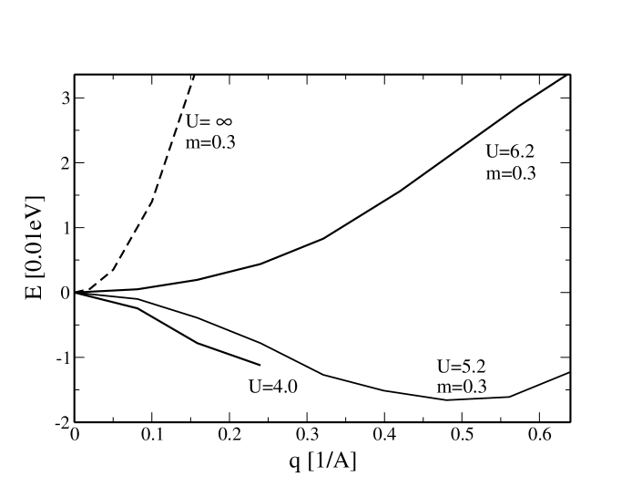
FIG. 2.: RPA spin-wave dispersion in $x$ direction, $E^{\text{RPA}}((q,0,0))$, for a generic two-band model with $n=0.3$ and $J=0.2U$. The value $U=4.0\,\text{eV}$ corresponds to $m<n$ in Hartree-Fock theory whereas $U=5.2\,\text{eV}$ and $U=6.2\,\text{eV}$ correspond to the fully polarized Hartree-Fock ground state. Also shown is the spin-wave dispersion for $U=\infty$. The lattice constant is $a=2.5\,$Å.

REFERENCES

• [1] Stoner E C 1938 Proc. Roy. Soc. A 165 372; Slater J C 1953 Rev. Mod. Phys. 25 199; Wohlfarth E P 1953 ibid., 211
• [2] Van Vleck J H 1953 Rev. Mod. Phys. 25 220
• [3] Gutzwiller M C 1963 Phys. Rev. Lett. 10, 159; 1964 Phys. Rev. 134, A923; 1965 Phys. Rev. 137 A1726
• [4] Herring C 1966 Magnetism Vol. IV, ed. by G T Rado and H Suhl (New York: Academic Press) p. 1
• [5] Morija T 1985 Spin Fluctuations in Itinerant Electron Magnetism (Berlin: Springer)
• [6] Capellmann H (Ed) 1986 Metallic Magnetism (Berlin: Springer)
• [7] Yosida K 1998 Theory of Magnetism (Berlin: Springer)
• [8] Fazekas P 1999 Lecture Notes on Electron Correlation and Magnetism (Singapore: World Scientific)
• [9] Eberhardt W and Plummer E W 1980 Phys. Rev. B 21 3245
• [10] Bünemann J, Gebhard F and Weber W 2000 Found. of Physics 30 2011
• [11] For a recent review, see Vollhardt D, Blümer N, Held K, Kollar M, Schlipf J, Ulmke M and Wahle J 1999 Adv. in Solid-State Physics 28 383
• [12] Ulmke M 1998 Eur. Phys. J. B 1 301; Tasaki H 1998 Prog. Theor. Phys. 99 489
• [13] Bünemann J, Weber W and Gebhard F 1998 Phys. Rev. B 57, 6896
• [14] Held K and Vollhardt D 1998 Eur. Phys. J. B 5, 473
• [15] Daul S and Noack R M 1998 Phys. Rev. B 58 2635; Guerro M and Noack R M 2001 Phys. Rev. B 63 144423
• [16] Sakamoto H, Momoi T and Kubo K 2001 (unpublished; arXiv cond-mat/0104223)
• [17] Bünemann J, Gebhard F and Weber W 1997 J. Phys. Cond. Matt. 8 7343
• [18] Nolting W (Ed) (forthcoming) Ground-State and Finite-Temperature Bandferromagnetism (Berlin: Springer)
• [19] Marshall W and Lovesey S W 1971 Theory of Thermal Neutron Scattering (Oxford: Oxford University Press)
• [20] Mook H A, Nicklow R M, Thompson E D and Wilkinson M K 1969 J. Appl. Phys. 40 1450; Lowde R D and Windsor C G 1970 Adv. Phys. 19 813
• [21] Cooke J F, Lynn J W and Davis H L 1980 Phys. Rev. B 21 4118
• [22] Tang H, Plihal M and Mills D L 1998 J. Magn. Magn. Matt. 187 23; Plihal M and D L Mills 1998 Phys. Rev. B 58 14407; Hong J and Mills D L 2000 Phys. Rev. B 61, R858
• [23] Uhl M and Kübler J 1996 Phys. Rev. Lett. 77 334; Rosengaard N M and Johansson B 1997 Phys. Rev. B 55 14975; Halilov S V, Eschrig H, Perlov A Y, and Oppeneer P M 1998 Phys. Rev. B 58, 293
• [24] Bünemann J 2001 J. Phys. Cond. Matt. 13 5327
• [25] Gebhard F 1997 The Mott Metal-Insulator Transition (Berlin: Springer)
• [26] Mahan G D 1990 Many-Particle Physics 2nd ed. (New York: Plenum Press)
• [27] Gebhard F 1990 Phys. Rev. B 41, 9452
• [28] Bünemann J, in preparation
Refer to caption