The charge and low-frequency response of normal-superconducting heterostructures

Abstract

The charge distribution is a basic aspect of electrical transport. In this work we investigate the self-consistent charge response of normal-superconducting heterostructures. Of interest is the variation of the charge density due to voltage changes at contacts and due to changes in the potential. We present response functions in terms of functional derivatives of the scattering matrix. We discuss corrections to the Lindhard function due to the proximity of the superconductor. We use these results to find the dynamic conductance matrix to lowest order in frequency. We illustrate similarities and differences between normal systems and heterostructures for specific examples like a ballistic wire, a resonator, and a quantum point contact.

PACS numbers: 72.10.Bg, 72.70.+m, 73.23.-b, 74.40+k

]

I Introduction

During the past decade mesoscopic systems consisting of both normal and superconducting parts have attracted considerable attention. Microscopically, the interesting physics stems from Andreev reflection. An incident particle is reflected as a hole and a Cooper pair is generated in the superconductor. This results in an effective charge transfer of $2e$ and correlations between Andreev reflected electron hole pairs (the proximity effect). These effects have been investigated in many experimental and theoretical works [1, 2] focusing mainly on the stationary transport regime (dc-conductance) [3, 4] and the low-frequency noise (shot noise) [5, 6]. The ac-regime has attracted much less attention [7, 8, 9, 10].

In an Andreev process the electron and hole parts of the wave function contribute with opposite charge. It is therefore interesting to investigate the low-frequency ac-transport of NS-systems, since this problem requires a electrically self-consistent discussion of the charge distribution in the sample. This self-consistency is of importance not only for ac-transport but also for the discussion of charge fluctuations and the non-linear transport regime [11].

In this work we have in mind the interplay of two main properties of hybrid structures: On one hand raising or lowering the voltage at a normal contact of the sample will not inject an additional charge into regions where the wave functions contain electron and hole amplitudes of equal magnitude. This is in strong contrast to a purely normal conductor! On the other hand screening is a property not only of the states at the Fermi surface but of the entire electron gas. Thus the ability of a hybrid structure to screen an additional charge is essentially the same as that of a normal conductor.

Our results show two main differences compared to purely normal systems: first, the coupling of carriers with opposite charge reduces the interaction with nearby gates. Second, Andreev reflection increases the dwell time inside the structure and this affects the ac-response.

The paper is organized as follows: In section II, we derive an expression of the charge density in terms of functional derivatives of the scattering matrix. We next discuss the charge density response to external and internal potential perturbations. In section IV we use these results to formulate a self-consistent theory of low-frequency ac-response. To illustrate our results we consider in section V a number of examples: a ballistic wire, a resonant structure and the quantum point contact connected to a superconductor.

II Charge Density

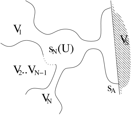
FIG. 1.: A mesoscopic scattering region is attached to $N$ normal reservoirs and one superconducting reservoir. It is described by two scattering matrices $s_{N}$ describing the normal conducting region and $s_{A}$ describing the Andreev reflection. Each terminal has its own bias voltage $V_{\alpha}$. The electrostatic potential $U$ inside the scatterer is calculated self-consistently.

In this section we derive the general expression for the charge density $\langle\hat{\rho}(r)\rangle$ in the scattering problem sketched in Fig. 1. A scattering region is attached to $N$ normal leads and one superconducting lead. Every normal lead is characterized by its applied voltage $V_{\alpha}$, the superconducting lead by its pair potential $\Delta$ and the bias $V_{S}$. For all the calculations we may choose $V_{S}=0$. The fact that we only allow for one superconducting terminal excludes all time-dependent Josephson-like effects. For an introduction to the applied formalism we refer the reader to Ref. [12]. The whole system is described by its scattering matrix

$$s_{\alpha\beta}=\left(\begin{array}[]{cc}s_{\alpha\beta}^{pp}&s_{\alpha\beta}^{ph}\\ s_{\alpha\beta}^{hp}&s_{\alpha\beta}^{hh}\\ \end{array}\right).$$ (1)

The element $s_{\alpha\beta}^{hp}$ for example is the current amplitude of a hole that leaves through lead $\alpha$ and has entered with unit current amplitude as a particle through lead $\beta$. We represent each scattering channel by its own lead to save two indices.

It is conceptually useful [13] to imagine the scattering matrix $s$ being assembled from a part that describes the reflection and transmission in the normal region $s_{N}^{p/h}$ and from a part that describes the Andreev processes at the interface between normal metal and superconductor $s_{A}$. Only this second matrix leads to coupling between the particle and hole scattering states. However, the following derivations do not depend on this assumption. For energies $E$ smaller than the gap energy $|\Delta|$ only reflection takes place at the interface. The total scattering matrix $s$ then has the dimension $(2N_{N})^{2}$ where $N_{N}=\sum N_{\alpha}$ is the total number of channels leading to normal reservoirs. Above the gap we must also include transmission processes, and therefore the dimension changes to $(2N+2N_{S})^{2}$. The superconducting terminal adds $N_{S}$ more channels.

For the following it is helpful to introduce local partial densities of states (LPDOS) [14]

$$\nu(\alpha_{\nu},r_{\kappa},\beta_{\mu})=-\frac{1}{2\pi q^{\kappa}}\text{Im}\left[(s_{\alpha\beta}^{\nu\mu})^{*}\frac{\delta s_{\alpha\beta}^{\nu\mu}}{\delta U^{\kappa}(r)}\right].$$ (2)

This expression is valid for one channel per lead. A true multichannel expression would include a trace over the channels. The value $\nu(1^{h},r^{p},2^{p})$ for example describes the density of particles at location $r$ that entered as particles through contact $2$ and leave as holes through lead $1$. In definition (2) we denote the quasi-particle charge by $q^{p/h}=\pm q$. The LPDOS must be calculated as functional derivatives of the scattering matrix with respect to the electrostatic potential $U$. To gain the information about particles and holes separately [14] we artificially split up the electrostatic potential $U$ in a part that acts on particles $U^{p}$ and another that addresses holes $U^{h}$. The Bogoliubov-de Gennes Hamiltonian then takes the form

$$\hat{H}=\left(\begin{array}[]{l}H_{0}+qU^{p}(x)-E_{F}\quad\Delta\\ \\ \Delta^{*}\quad-(H_{0}+qU^{h}(x)-E_{F})^{*}\\ \end{array}\right).$$ (3)

These equations have to be solved including a small variation of the electrostatic potentials $U^{p}$ and $U^{h}$ in order to get the scattering matrix and its functional derivatives.

The above defined LPDOS are not independent. On one hand, the LPDOS obey reciprocity relations. This has been investigated in reference [14]. On the other hand the particle-hole symmetry of the Bogoliubov-de Gennes equation implies

$$\nu(\alpha_{\nu},r_{\kappa},\beta_{\mu},E)=\nu(\alpha_{\bar{\nu}},r_{\bar{\kappa}},\beta_{\bar{\mu}},-E).$$ (4)

The bar denotes the opposite ($p/h=\bar{h}/\bar{p}$). Both symmetries can be used to reduce the expense of the calculation.

The charge density inside the normal-superconducting heterostructure can be entirely expressed by the LPDOS (and therefore by the scattering matrix) and the occupation factors of the attached reservoirs

$$\begin{array}[]{l}\langle\hat{\rho}(r)\rangle=q\int_{-\infty}^{\infty}dE\sum_{\alpha\beta\mu\nu}\\ \\ \quad\left(f_{\beta}^{\mu}(E)\nu(\alpha_{\nu},r_{p},\beta_{\mu})+(1-f_{\beta}^{\mu}(E))\nu(\alpha_{\nu},r_{h},\beta_{\mu})\right).\end{array}$$ (5)

The occupation factors include the bias voltage of the normal terminals $f_{\beta}^{p/h}(E)=f(E-q^{p/h}V_{\beta})$. Here $f$ is the Fermi function. Note that the occupation factors vary in opposite directions for particles and holes. In Eq. (5) we have double counted the particle-hole excitations and hence drop a factor of two for spin degeneracy. The derivation of this result is outlined in appendix A.

III Charge Response and Gauge Invariance

Given formula (5) we are now in a position to calculate the charge density response $\delta\rho(r)$ to both internal and external potential variations

$$\delta\rho(r)=\sum_{\beta=S,1..N}\frac{\partial\rho(r)}{\partial V_{\beta}}\delta V_{\beta}-\int dr^{\prime}\tilde{\Pi}(r,r^{\prime})\delta U(r^{\prime}).$$ (6)

The first contribution is the bare charge injected from the leads due to the shift of the occupation factors, and is proportional to the injectivities $\partial\rho(r)/\partial V_{\beta}$. The second contribution arises from the change of the internal potential due to screening (the potential itself will be determined in the following subsection), and involves the Lindhard function $\tilde{\Pi}(r,r^{\prime})=-\partial\rho(r)/\partial U(r^{\prime})$.

The injectivity from the normal leads can be calculated straightforwardly from the charge density (5)

$$\frac{\partial\rho(r)}{\partial V_{\beta}}=\int dE\left(-\frac{\partial f}{\partial E}\right)\sum_{\alpha\nu\mu\kappa}q^{\kappa}q^{\mu}\nu(\alpha_{\nu},r_{\kappa},\beta_{\mu})$$ (7)

and depends at low temperatures as expected only on properties at the Fermi energy. The other quantities contained in the balance equation (6) need a more careful analysis. Its technical details are explained in appendix B.

The procedure of calculating the non-local Lindhard function $\tilde{\Pi}(r,r^{\prime})$ leads to second order functional derivatives that cannot be simplified further. However, if we assume the Lindhard function to be local, $\tilde{\Pi}(r,r^{\prime})=\delta(r-r^{\prime})\Pi(r)$, we can express it by the above calculated LPDOS (2). This assumption is correct if the electrostatic potential varies only slowly on the scale of the Fermi wavelength $\lambda_{F}$. To express the result in a transparent way we split up the energy $E$ in the same way as the potential $U(r)$. We introduce the quantities $E^{p/h}$ that denote the energy dependence of the scattering matrices for particles and holes $s_{N}^{p/h}(E^{p/h})$. Furthermore we need a critical energy $E_{c}$ with the property $|\Delta|\ll E_{c}\ll E_{F}$. Such an energy is useful, since particles and holes with energies outside the range $[-E_{c},E_{c}]$ have a negligible Andreev reflection probability that decays as $\sim|\Delta|^{2}/E^{2}$. In a short calculation given in appendix B we find for the local Lindhard function

$$\begin{array}[]{ll}\Pi(r)=&q^{2}\sum_{\alpha\beta}\left[\nu(\alpha_{p},r_{p},\beta_{p},-E_{c})+\nu(\alpha_{h},r_{h},\beta_{h},+E_{c})\right]\\ \\ &+q^{2}\int_{-E_{c}}^{+E_{c}}dE\sum_{\alpha\beta\mu\nu}\left.\left(\frac{\partial}{\partial E^{p}}-\frac{\partial}{\partial E^{h}}\right)\right|_{E^{p},E^{h}=E}\\ \\ &\left[f(E)\nu(\alpha_{\nu},r_{p},\beta_{\mu})+f(-E)\nu(\alpha_{\nu},r_{h},\beta_{\mu})\right].\\ \end{array}$$ (8)

If the local electrostatic potential $U(r)$ fulfills the condition $E_{F}-U(r)\gg|\Delta|$ the first line of Eq. (8) dominates. Therein we can replace the sum over the LPDOS by the local density of states at $E=0$ for the equivalent normal conducting structure. This is the expression for the Thomas-Fermi screening in a purely normal sample. The screening properties are not affected by the presence of the superconductor. Our result becomes more interesting for $E_{F}-U(r)\sim|\Delta|$ when the second and third term of Eq. (8) contribute significantly. We later illustrate this case with a specific example.

A simple argument allows us to get the injectivity from the superconducting terminal $\partial\rho(r)/\partial V_{S}$ without any further calculation. The Bogoliubov-de Gennes equations are gauge invariant, a simultaneous change of all external and internal potentials by the same amount will not lead to any charge inside the system. Setting the left side of Eq. (6) to zero gives therefore

$$\Pi(r)=\sum_{\beta=S,1..N}\frac{\partial\rho(r)}{\partial V_{\beta}}.$$ (9)

Since $\Pi(r)$ and the injectivities of all normal contacts are known we can use this relation to find the injectivity $\partial\rho(r)/\partial V_{S}$ of the superconducting contact.

IV Linear Response Calculation

In order to get the low-frequency ac-response of our system it is necessary to distinguish two contributions to the current. On one hand we have the current flow $I^{bare}$ of non interacting particles which can be accessed by a linear response theory. On the other hand we may not neglect the screening currents $I^{scr}$ due to interactions. The low-frequency conductance matrix can be generally written as

$$G_{\alpha\beta}=\frac{\partial\langle I_{\alpha}\rangle}{\partial V_{\beta}}=G_{\alpha\beta}^{0}-i\omega E_{\alpha\beta},$$ (10)

where the ”emittance” matrix $E$ consists of two parts $E=E^{bare}+E^{scr}$.

The screening currents may be calculated quasi-statically solving a Poisson equation self-consistently. This procedure is described in detail in reference [15]. Here we cite only the result

$$E_{\alpha\beta}^{scr}=-\int drdr^{\prime}g(r,r^{\prime})\frac{\partial\rho(r)}{\partial V_{\alpha}}\frac{\partial\rho(r^{\prime})}{\partial V_{\beta}},$$ (11)

which is valid in the presence of time reversal symmetry. The kernel $g(r,r^{\prime})$ is given by $\int dr^{\prime\prime}4\pi\tilde{\Pi}(r,r^{\prime\prime})g(r^{\prime\prime},r^{\prime})-\nabla^{2}_{r}g(r,r^{\prime})=4\pi\delta(r-r^{\prime})$. In a discretized model the Laplace-operator may be replaced by a capacitance matrix.

To find the bare contribution $E^{bare}$ to the emittance we proceed as in reference [16]. We use the current operator at the normal conducting terminal $\alpha$

$$\begin{array}[]{ll}\hat{I}_{\alpha}=&\frac{1}{h}\sum_{\beta\beta^{\prime}vww^{\prime}}q^{v}\int dEdE^{\prime}e^{+i(E-E^{\prime})t/\hbar}\\ \\ &\hat{a}_{\beta}^{w\dagger}(E)\hat{a}_{\beta^{\prime}}^{w^{\prime}}(E^{\prime})\times A_{\beta\beta^{\prime}}^{ww^{\prime}}(\alpha,v,E,E^{\prime}),\\ \end{array}$$ (12)

in a simplified form valid in the low-frequency limit. The full current operator has been given for example in reference [17]. In Eq. (12) the indices $\alpha,\beta,\beta^{\prime}$ denote leads (and channels), $v,w,w^{\prime}$ distinguish particle and hole states. The operator $\hat{a}_{1}^{h}(E)$ for example creates a hole of energy $E$ incident into lead $1$. The matrix elements $A$ are given by

$$A_{\beta\beta^{\prime}}^{ww^{\prime}}(\alpha_{v},E,E^{\prime})=\delta_{\alpha\beta}\delta_{\alpha\beta^{\prime}}\delta_{vw}\delta_{vw^{\prime}}-\left(s_{\alpha\beta}^{vw}(E)\right)^{*}s_{\alpha\beta^{\prime}}^{vw^{\prime}}(E^{\prime}).$$ (13)

The ac-conductivity can then be obtained from

$$g_{\alpha\alpha^{\prime}}=\frac{1}{\hbar\omega}\int_{0}^{\infty}d\tau e^{i(\omega+i\delta)\tau}\langle\left[\hat{I}_{\alpha}(\tau),\hat{I}_{\alpha^{\prime}}(0)\right]\rangle.$$ (14)

The evaluation of the commutator is mostly straight forward. As in previous works [16] we use the unitarity of the scattering matrix and the thermal occupation of the reservoirs. As in the case of a purely normal system we are left with a doubled energy integral. We can evaluate this integral through a path deformation in the upper complex plane where the scattering matrix is analytical. In the end we expand the result up to first order in frequency. The result for the dc-conductance

$$G_{\alpha\beta}^{0}=\frac{1}{h}\int dE\left(-\frac{\partial f}{\partial E}\right)\sum_{\mu\nu}q^{\mu}q^{\nu}\left[\delta_{\alpha\beta}\delta_{\mu\nu}-T_{\alpha\beta}^{\mu\nu}\right]\\$$ (15)

is identical to the one established in the literature [17, 18, 13, 19]. This serves as a check of our calculation. In Eq. (15), $T_{\alpha\beta}^{\mu\nu}=(s_{\alpha\beta}^{\mu\nu})^{*}s_{\alpha\beta}^{\mu\nu}$ is the transmission probability from channel $\beta$ to channel $\alpha$. The bare emittance can be expressed by global partial densities of states (GPDOS)

$$N(\alpha_{\nu},\beta_{\mu})=\frac{1}{2\pi}\text{Im}\left(s_{\alpha\beta}^{\nu\mu}\right)^{*}\frac{\partial s_{\alpha\beta}^{\nu\mu}}{\partial E},$$ (16)

and becomes

$$E^{bare}_{\alpha\beta}=\int dE\left(-\frac{\partial f}{\partial E}\right)\sum_{\nu\mu}q^{\nu}q^{\mu}N(\alpha_{\nu},\beta_{\mu}).$$ (17)

This equation shows that the bare emittance may change its sign. This simple calculation provides only the emittance matrix elements between normal terminals. A direct calculation of the current at the superconducting reservoir would involve a self-consistent evaluation of the pair potential in the superconductor. Its phase “carries” the supercurrent. Nevertheless, the missing elements of the emittance matrix can be reconstructed from the conditions

$$\sum_{\alpha}E_{\alpha\beta}=\sum_{\beta}E_{\alpha\beta}=0$$ (18)

that express current and charge conservation.

V Examples

We now present some simple calculations to illustrate how the presence of a superconducting terminal affects the ac-properties of a mesoscopic sample. We emphasize that these examples are not designed to model a realistic sample completely, but should exhibit qualitatively the main features.

A Ballistic Wire

As a first example we discuss briefly the emittance of a ballistic wire with one open channel at zero temperature. The results can be easily generalized to more than one channel. The geometry of the sample is shown in Fig. 2. The wire is attached to two reservoirs ($1,2$). Reservoir $1$ is always normal conducting. The second may be normal conducting, superconducting or completely disconnected from the wire for comparison.

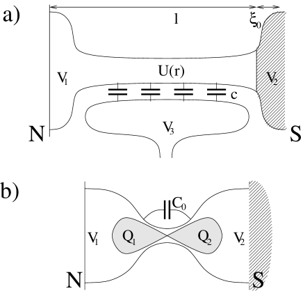
FIG. 2.: Examples: a) A one channel ballistic wire is attached to a superconductor. Its length is denoted by $\ell$, the internal interaction modeled by a capacitance per unit length $c$ between wire and gate. The emittance is enhanced by a factor of $4$ compared to a purely normal wire. b) The same geometry for a quantum point contact which is described by an electrostatic dipole of capacitance $C_{0}$. In the low transparency limit the ac-conductance is dominated by the geometric capacitance $C_{0}$. In the opposite limit the quantum point contact shows enhanced inductive behaviour.

The wire is described by its length $\ell$ and the dimensionless parameter $a=4q^{2}/hv_{F}$ which describes the DOS at the Fermi level in the wire. Note that $a$ is also the local Lindhard function of Eq. (8). The interaction in the wire is modeled by a third gate terminal ($3$). It is coupled to the wire by a geometrical capacitance per unit length $c$ and assumed to be macroscopic. Thus we can replace the Laplace operator in Eq. (11) by $-4\pi c$. For a detailed description of this system see for example [20].

	normal conducting	superconducting	disconnected
$E_{11}$	$-\frac{a^{2}\ell}{4(c+a)}$	$-a(\ell+\xi_{0}/2)$	$\frac{ac\ell}{(c+a)}$
$E_{12}$	$\frac{a\ell(a+2c)}{4(c+a)}$	$a(\ell+\xi_{0}/2)$	$0$
$E_{22}$	$-\frac{a^{2}\ell}{4(c+a)}$	$-\frac{a^{2}\ell}{(c+a)}-a\xi_{0}/2$	$0$

TABLE I.: Comparison of the emittance elements of a ballistic wire connected to two normal reservoirs, a normal and a superconducting reservoir and to one normal reservoir only.

As a last parameter we need the coherence length of the superconductor $\xi_{0}=\hbar v_{F}/|\Delta|$. We neglect the self-consistency of its pair potential.

Table I summarizes the results for the three cases. The missing elements of the emittance matrix can be reconstructed from Eq. (18). We add some observations to explain the differences between the results. The response of the disconnected wire is purely capacitive, while the open wires act inductively. In the limit of charge neutrality $c\ll a$ the inductive emittance of an open wire $E_{11}$ grows by a factor of four in the presence of a superconductor. On one hand the bare emittance is doubled, because an incoming electron leaving as an Andreev reflected hole stays twice as long in the wire. On the other hand this effect is not weakened by a capacitive screened emittance, because the injectivity from the normal lead into the wire $\partial\rho/\partial V_{1}$ is zero. This leads to another factor of two. Additionally, the evanescent quasi-particle wave contributes to the bare emittance, the wire acquires an effective length $\ell+\xi_{0}/2$ (we use the assumption that the Fermi velocities are the same on both sides of the NS-interface).

The emittance $E_{13}=-E_{11}-E_{12}$ is always zero in the presence of a superconductor. The gate and the normal terminal are only connected via the capacitance. But this capacitance cannot be charged from the normal side $1$ because the above mentioned injectivity $\partial\rho/\partial V_{1}$ is zero. Every injected electron comes back as a hole that compensates its charge. Therefore, the ac-response to a bias at the normal end must be zero. Vice versa the capacitive element $E_{23}$ becomes twice as big because of a doubled injectivity $\partial\rho/\partial V_{2}$ in the limit of potential neutrality $c\gg a$.

B Resonator

As briefly discussed after Eq. (8) we expect the internal charge response to be very different from a purely normal system, if the states inside the superconducting gap give the dominant contribution to the Lindhard function. To further investigate this point we now consider the charge on a series of resonances of Breit-Wigner type coupled to a superconductor. For analytical simplicity we take the resonances equidistant. A single resonance of this kind is discussed for example in [21]. Its experimental equivalent might be a level on a quantum dot which is coupled to one normal and one superconducting lead through tunneling barriers. However, this situation is normally treated in a Coulomb blockade picture where the strongly fluctuating electrostatic potential is treated as an operator. In our theory the potential becomes a c-number. Therefore, this model is limited to the case of a small charging energy.

The resonances are described by the following scattering matrix in the normal part

$$s_{N,ij}=\delta_{ij}-i\pi\frac{\sqrt{\Gamma_{i}\Gamma_{j}}}{\Delta_{L}}\cot\pi\frac{E-qU+i(\Gamma_{N}+\Gamma_{S})/2}{\Delta_{L}}.$$ (19)

The coupling width of the resonances to the normal lead is $\Gamma_{N}$, to the superconducting lead it is $\Gamma_{S}$. The level spacing on the resonator is given by $\Delta_{L}$. The above given scattering matrix is only unitary in the limit $\Gamma_{N/S}\ll\Delta_{L}$ which means for small coupling.

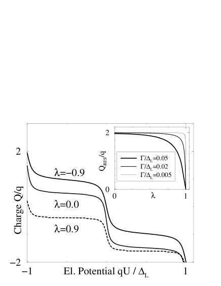
FIG. 3.: A resonator with level spacing $\Delta_{L}$ is attached to a normal and a superconducting wire with resonance widths $\Gamma_{N/S}$ respectively. Their average is called $\Gamma=(\Gamma_{S}+\Gamma_{N})/2$, the parameter $\lambda=(\Gamma_{S}-\Gamma_{N})/(\Gamma_{S}+\Gamma_{N})$ describes their relation. The big plot shows the charge $Q$ on the resonator as a function of its electrostatic potential $U$ for different parameters $\lambda$. The lineshape changes (see Eq. (21)), and for increasing $\lambda$ the charging decreases. This is illustrated in the inset that shows the charge per resonance $Q_{RES}$ as a function of $\lambda$.

This scattering matrix is periodic in the energy $E$ and the integrals in the equation for the charge density (5) diverge. We therefore introduce a cutoff $E_{min}$ by hand that defines the lowest level on the resonator. This cutoff lies still inside the energy range of the superconducting gap $|E_{min}|\ll|\Delta|$. This allows us to use the scattering matrix

$$s_{A}=\left(\begin{array}[]{cc}s^{pp}&s^{ph}\\ s^{hp}&s^{hh}\end{array}\right)=\left(\begin{array}[]{cc}0&-i\\ -i&0\end{array}\right)$$ (20)

to describe the Andreev reflection. This example is now constructed in such a way that the correction of the Lindhard function due to the presence of the superconductor (second term in Eq. (8)) becomes very important. Fig. 3 shows a numerical evaluation of the charge on the resonator $Q$ as a function of the electrostatic potential $U$ on the resonator. We describe the coupling by a parameter $\lambda=(\Gamma_{S}-\Gamma_{N})/(\Gamma_{S}+\Gamma_{N})$. This parameter gets $1$ if the resonance is only connected to the superconductor and $-1$ in the opposite case. The inset if Fig. 3 illustrates the charge stored on one resonance $Q_{RES}$ as a function of $\lambda$. This charge is $2q$ if the resonator is charged only from the normal side (we assume spin degeneracy, this is the point where the Coulomb blockade gives a completely different picture). If the resonator is only connected to the superconductor no charge can be transferred at all. Below the superconducting gap $|\Delta|$ the states in the resonator are equally weighted superpositions of particle and hole states that cannot contribute to the charging of the resonator.

It is worth to note, that the shape of the steps in Fig. 3 changes as a function of $\lambda$. In the two different limits we obtain

$$\begin{array}[]{ll}Q_{N}=-q\frac{2}{\pi}\text{arctan}\frac{2qU}{\Gamma_{N}}&\Gamma_{N}\gg\Gamma_{S},\\ \\ Q_{S}\propto-q\frac{2qU}{\sqrt{(2qU)^{2}+\Gamma_{S}^{2}}}&\Gamma_{S}\gg\Gamma_{N}.\end{array}$$ (21)

These results are valid at zero temperature. For $kT>\Gamma_{N/S}$ the steps are smeared out by the Fermi function.

C Quantum Point Contact

The low-frequency conductance of a quantum point contact (QPC) connecting two normal leads has been studied in Ref. [22]. We adapt this procedure to our situation sketched in Fig. 2. In a first step we only consider one transmission channel. We assume the QPC is described by a symmetric equilibrium potential. At equilibrium the only asymmetry stems from the presence of the superconducting lead. Polarization of the QPC due to an applied voltage leads to a dipole. (Charging vis-avis the gates is neglected. See however Ref. [23]). The size of this dipole is described by one single capacitance $C_{0}$. Furthermore, we limit ourselves to a semiclassical treatment which essentially means that the confining potential is sufficiently expanded in space. In this limit the second and third part of Eq. (8) are negligible. As a second parameter we need the total density of states at the Fermi level (over a region in which the charge is not screened fully), when the system is entirely normal $D^{N}=q^{2}N_{F}$. In addition, scattering at the QPC is characterized by its transmission probability $T$ and its reflection probability $R=1-T$. As shown in [22] the electrochemical capacitance and the emittance in the purely normal system are

$$C^{N}=R\frac{C_{0}D^{N}}{4C_{0}+D^{N}},\quad E^{N}=RC^{N}-\frac{D^{N}}{4}T^{2}.$$ (22)

This result uses the fact that the semiclassical injectivities may be written as

$$\frac{\partial Q^{N}_{1}}{\partial V_{1}}=\frac{D^{N}}{4}\left(1+R\right),\quad\frac{\partial Q^{N}_{2}}{\partial V_{1}}=\frac{D^{N}}{4}\left(1-R\right).$$ (23)

For example, the response $\partial Q^{N}_{1}/\partial V_{1}$ originates from all the right going electrons in region $1$ plus the left going ones that have been reflected at the barrier.

It is clear that this picture will change drastically in the presence of a superconductor. We denote by $R_{N}=4R/(1+R)^{2}$ the probability that an electron is scattered back as an electron. The probability for Andreev reflection we call $R_{A}=1-R_{N}=T^{2}/(1+R)^{2}$. The dc-conductance is of course $4R_{A}q^{2}/h$. The injectivities now turn out to be

$$\frac{\partial Q^{S}_{1}}{\partial V_{1}}=\frac{D^{N}}{2}R_{N},\quad\frac{\partial Q^{S}_{2}}{\partial V_{1}}=0,\,$$ (24)

$$\frac{\partial Q^{S}_{1}}{\partial V_{2}}=\frac{D^{N}}{2}R_{A},\quad\frac{\partial Q^{S}_{2}}{\partial V_{2}}=\frac{D^{N}}{2}.$$ (25)

For example in $\partial Q^{S}_{1}/\partial V_{1}$, we recognize that only the electrons that return as electrons contribute to the injectivity. We see also that the normal terminal cannot inject charge into the right side of the QPC which is also clear from intuition.

Now we use these ingredients to find the capacitance and emittance of the whole QPC. For simplicity, we cite the results without the length renormalization due to a finite $\xi_{0}$ in the superconductor. We find

$$C^{S}=R_{N}\frac{C_{0}D^{N}}{4C_{0}+D^{N}},$$ (26)

$$E^{S}=R_{N}C^{S}-\frac{T(1-4R-R^{2})}{(1+R)^{4}}D^{N}.$$ (27)

In the low transparency limit ($R\simeq 1$) the result is the same as for the purely normal conducting system (22). In the high transparency limit ($R\simeq 0$) we recover the inductive behaviour of example V A. Again the emittance is increased by a factor of four in comparison to the result (22).

Fig. 4 shows a qualitative comparison of the conductance, capacitance and emittance of a multichannel QPC in the two geometries. We use a capacitance of $C_{0}=1\text{fF}$ and a potential $U(x)=\text{max}\{V_{0}(\lambda^{2}-x^{2}),0\}$ where $\lambda=500\text{nm}$. The constriction in y-direction allows up to five open channels with equidistant spacing through the contact.

What are the restrictions of the results obtained for our simple model system? The assumption that the NS-interface is a perfect Andreev mirror seems to play the most important role. In this case we may neglect the capacitance of the NS-interface. If such a capacitance would be present it would decrease the inductive behaviour at high transparency.

FIG. 4.: Comparison between transport properties of a multichannel quantum point contact either attached to a normal lead (narrow line) or a superconducting lead (broad line). In the presence of the superconductor, its dc-conductance is doubled and the low-frequency ac-response is enhanced by a factor of four in the transparent limit. The curves are calculated in a WKB-approximation. The used parameters are specified in the text.

VI Conclusions

In this work we have extended the ac-response theory of normal mesoscopic conductors to hybrid normal and superconducting structures. This requires an investigation of screening and a discussion of the charge density response to external lead voltages in the presence of Andreev scattering. Global gauge invariance is valid also for the hybrid structures investigated here. This leads necessarily to the existence of an injectivity of the superconductor into the normal part of the structure. The charge-injectivity of the superconductor compensates the suppression of the charge-injectivity from a normal contact.

Screening in hybrid structures is up to small corrections the same as in normal conductors. Nevertheless, the ac-response of hybrid structures exhibits marked differences from that of a purely normal system. For a ballistic wire at one end connected to a superconducting reservoir, the emittance is four times as large as that of a purely normal wire. Furthermore, the displacement current induced into a nearby gate in response to an oscillating voltage at the normal contact (described by an off-diagonal capacitance element) is highly suppressed compared to the purely normal structure. For a resonant structure, the charge response to an internal variation of the electrostatic potential can be reduced due to the superposition of particle and hole states inside the cavity. A quantum point contact attached to a superconductor shows the same capacitive behavior as its normal conducting analog in the limit of small transmission. For high transmission the emittance is enhanced as in the case of a ballistic wire.

For the ac-conductance problem screening is necessary if we want to find a response that depends only on voltage differences and which conserves current. We have focused on geometries with a single NS-interface but similar considerations should apply if we deal with SNS-structures or more complicated geometries. Electrical self-consistency is relevant not only for dynamic problems but also if we are interested in non-linear transport or even just in the gate voltage dependence of stationary transport quantities. Therefore, the considerations presented should be useful for a wide range of geometries and for the investigation of many different physical problems.

A Charge Density

This is a short sketch of the derivation of formula (5). We express the expectation value of the charge density operator with help of the normalized solutions $(w_{\beta}^{\mu}(r,E))^{\dagger}=((u_{\beta}^{\mu}(r,E))^{*},(v_{\beta}^{\mu}(r,E))^{*})$ of the Bogoliubov-de Gennes equation [12]

$$\langle\hat{\rho}\rangle=q\sum_{\beta\mu}\int^{+\infty}_{-\infty}dE(w_{\beta}^{\mu})^{\dagger}\left(\begin{array}[]{cc}f_{\beta}^{\mu}&\\ &1-f_{\beta}^{\mu}\end{array}\right)w_{\beta}^{\mu}.$$ (A1)

The solutions of the Bogoliubov-de Gennes equation are scattering states in our case. We include the usual prefactors containing the group velocities in the normalization factors of the wavefunctions. Their mean occupation number can be expressed by the Fermi functions of the reservoirs $f_{\beta}^{p/h}(E)=f(E-q^{p/h}V_{\beta})$ depending on whether they describe an incoming particle $p$ or hole $h$. $q^{p/h}=\pm q$ denotes their quasi-particle charge.

The starting point of the calculation is the Bogoliubov-de Gennes equation (3). For the moment we allow the electrostatic potentials $U^{p/h}$ to be complex. The continuity equation for the quasi-particle current $j_{\alpha\beta}^{\mu}$ then reads

$$\nabla j_{\beta}^{\mu}=\frac{2q}{\hbar}\left[\text{Im}(U^{p})\left|u_{\beta}^{\mu}\right|^{2}+\text{Im}(U^{h})\left|v_{\beta}^{\mu}\right|^{2}\right].$$ (A2)

The complex potentials generate source terms on the right side of Eq. (A2). As a next step we integrate this equation over the volume of the scatterer. To this end we choose the potentials to vary like $U^{p/h}=U^{p/h}_{0}+i\Gamma^{p/h}\delta(x-x_{0})$. We then get for the current

$$I_{\beta,out}^{\mu}-I_{\beta,in}^{\mu}=\frac{2q}{\hbar}\left[\Gamma^{p}\left|u_{\beta}^{\mu}(x_{0})\right|^{2}+\Gamma^{h}\left|v_{\beta}^{\mu}(x_{0})\right|^{2}\right].$$ (A3)

In this equation we call $I_{in/out}$ the total current flow into and out of the scattering region. Their difference is not zero because of the source term in Eq. (A2). The ratio of both quantities can be expressed by the scattering matrix $s$

$$\frac{I_{\beta,out}^{\mu}}{I_{\beta,in}^{\mu}}=\sum_{\alpha\nu}\left(s_{\alpha\beta}^{\nu\mu}\right)^{*}s_{\alpha\beta}^{\nu\mu}.$$ (A4)

The scattering matrix is a functional of the small complex variation $\Gamma_{p/h}$ and thus can be expanded up to first order. To evaluate the incoming current $I_{in}$ we use the normalization of the wave functions $w_{\beta}^{\mu}$ and get $I_{\beta,in}^{\mu}=1/h$. Finally we manage to express the square of the wave functions by the LPDOS given in definition (2)

$$\sum_{\alpha\nu}\nu(\alpha_{\nu},r_{p},\beta_{\mu})=\left|u_{\beta}^{\mu}(r)\right|^{2},$$ (A5)

$$\sum_{\alpha\nu}\nu(\alpha_{\nu},r_{h},\beta_{\mu})=\left|v_{\beta}^{\mu}(r)\right|^{2}.$$ (A6)

These quantities can be inserted into Eq. (A1) to get the final result (5) given at the beginning of the article.

B Lindhard Function

In this appendix we explain the derivation of the local Lindhard function (LLF) given in Eq. (8). The nonlocal Lindhard function (NLF) is given by $\tilde{\Pi}(r,r^{\prime})=-\delta\rho(r)/\delta U(r^{\prime})$. We define functional potential derivatives of the LPDOS as follows

$$\chi_{\alpha\beta}^{\mu\nu}(r_{\kappa},r^{\prime}_{\lambda})=\frac{\delta\nu(\alpha_{\nu},r_{\kappa},\beta_{\mu})}{\delta U^{\lambda}(r^{\prime})}.$$ (B1)

Using this definition and Eq. (5) we can write the NLF as

$$\begin{array}[]{ll}\tilde{\Pi}=&-q\int_{-\infty}^{\infty}dE\sum_{\alpha\beta\mu\nu\lambda}\\ \\ &\left(f(E)\chi_{\alpha\beta}^{\mu\nu}(r_{p},r^{\prime}_{\lambda})+f(-E)\chi_{\alpha\beta}^{\mu\nu}(r_{h},r^{\prime}_{\lambda})\right).\end{array}$$ (B2)

The NLF is not a Fermi surface quantity but depends on all energies within the conduction band. The LLF is a good approximation if the electrostatic potential $U$ varies slowly on the scale of the Fermi wavelength. Under these circumstances the spatial integration appearing for example in Eq. (6) can be simplified

$$\int dr^{\prime}\tilde{\Pi}(r,r^{\prime})\delta U(r^{\prime})=\delta U(r)\int dr^{\prime}\tilde{\Pi}(r,r^{\prime})=\delta U(r)\Pi(r).$$ (B3)

To get the LLF we must therefore integrate the NLF over its second spatial variable $r^{\prime}$. Because of particle-hole symmetry it is sufficient to keep the first part of Eq. (B2). We may thus write the LLF in the following way

$$\Pi=-2q\left(\int\limits_{-\infty}^{-E_{c}}+\int\limits_{-E_{c}}^{+\infty}\right)dEf(E)\sum_{\alpha\beta\nu\mu\lambda}\int dr^{\prime}\chi_{\alpha\beta}^{\mu\nu}(r_{p},r^{\prime}_{\lambda}),$$ (B4)

where we used an energy scale $E_{c}$ with the property $|\Delta|\ll E_{c}\ll E_{F}$. Below $-E_{c}$ we may neglect any Andreev reflection. In this case there is no coupling between particle and hole states and all ’crossed’ LPDOS and the functional derivative $\delta/\delta U^{h}(r^{\prime})$ vanish. We may furthermore use

$$\frac{\partial}{\partial E_{p}}=-\int dr^{\prime}\frac{\delta}{q\delta U_{p}(r^{\prime})},\quad\frac{\partial}{\partial E_{h}}=+\int dr^{\prime}\frac{\delta}{q\delta U_{h}(r^{\prime})}.$$ (B5)

which holds in WKB-approximation and $\partial/\partial E^{p}=d/dE$ to get

$$\int dr^{\prime}\chi_{\alpha\beta}^{\mu\nu}(r_{p},r^{\prime}_{\lambda})\simeq\delta_{p\nu}\delta_{p\mu}\delta_{p\lambda}\left(-\frac{d}{dE}\right)\nu(\alpha_{p},r_{p},\beta_{p}).$$ (B6)

The second integral may similarly be simplified using Eq. (B5). Applying partial integration with respect to the energy we get the result presented in Eq. (8).

REFERENCES

- [1] G. E. Blonder, M. Tinkham, and T. M. Klapwijk, Phys. Rev. B 25, 4515 (1982).
- [2] Special issue on Mesoscopic Superconductivity, Superlattices and Microstruct. 25, No. 5/6, (1999).
- [3] S. G. den Hartog, C. M. A. Kapteyn, B. J. van Wees, and T. M. Klapwijk, Phys. Rev. Lett. 77, 4954 (1996).
- [4] P. Charlat, H. Courtois, Ph. Gandit, D. Mailly, A. F. Volkov, and B. Pannetier, Phys. Rev. Lett. 77, 4950 (1996).
- [5] X. Jehl and M. Sanquer, Phys. Rev. B 63, 52511 (2001).
- [6] T. Hoss, C. Strunk, T. Nussbaumer, R. Huber, U. Staufer, and C. Schönenberger, Phys. Rev. B 62, 4076 (2000).
- [7] A. F. Volkov and H. Takayanagi, Phys. Rev. Lett 76, 4026 (1996).
- [8] V. N. Antonov and H. Takayanagi, Phys. Rev. B 56, R8515 (1997).
- [9] A. A. Kozhevnikov, R. J. Schoelkopf, and D. E. Prober, Phys. Rev. Lett 84, 3398 (2000).
- [10] J. Wang, Y. Wei, H. Guo, Q. Sun, and T. Lin, cond-mat/0011150 (2000).
- [11] A. M. Martin, Th. Gramespacher, and M. Büttiker, Phys. Rev. B 60, R12581 (1999). A. M. Martin, Th. Gramespacher, and M. Büttiker, J. Phys. Condensed Matter 11, L565 (1999). Screening in these works is treated incorrectly, and should be described using the results presented here.
- [12] S. Datta, Ph. Bagwell and M. P . Anantram, Phys. Low-Dim. Struct. 3, 1-102 (1996).
- [13] M. J. M. de Jong and C. W. J. Beenakker, Phys. Rev. B 49, 16070 (1994).
- [14] Th. Gramespacher, and M. Büttiker, Phys. Rev. B 61, 8125 (2000).
- [15] M. Büttiker, J. Math. Phys. 37, 4793 (1996)
- [16] M. Büttiker, A. Prêtre, and H. Thomas, Phys. Rev. Lett. 70, 4114 (1993).
- [17] M. P. Anantram and S. Datta, Phys. Rev. B 53, 16390 (1996).
- [18] Y. Takane and H. Ebisawa, J. Phys. Soc. Jpn. 61, 2858 (1992).
- [19] C. J. Lambert, V. C. Hui, and S. J. Robinson, J. Phys. Condensed Matter 5, 4187 (1993).
- [20] Ya. M. Blanter, F. W. J. Hekking, and M. Büttiker, Phys. Rev. Lett. 81, 1925 (1998).
- [21] C. W. J. Beenakker, in Mesoscopic quantum physics, edited by E. Akkermans et al, Elsevier Science B.V., Holland, 279 (1995).
- [22] T. Christen and M. Büttiker, Phys. Rev. Lett. 77, 143 (1996).
- [23] M. Büttiker and T. Christen, in ”Mesoscopic Electron Transport”, NATO Advanced Study Institute, Series E: Applied Science, edited by L. L. Sohn, L. P. Kouwenhoven and G. Schoen, (Kluwer Academic Publishers, Dordrecht, 1997). Vol. 345. p. 259.