Single-hole dynamics in the half-filled two-dimensional Kondo-Hubbard model.

Abstract

We consider the Kondo lattice model in two dimensions at half filling. In addition to the fermionic hopping integral $t$ and the superexchange coupling $J$ the role of a Coulomb repulsion $U$ in the conduction band is investigated. We find the model to display a magnetic order-disorder transition in the $U$-$J$ plane with a critical value of $J_{c}$ which is decreasing as a function of $U$. The single particle spectral function $A(\vec{k},\omega)$ is computed across this transition. For all values of $J>0$, and apart from shadow features present in the ordered state, $A(\vec{k},\omega)$ remains insensitive to the magnetic phase transition with the first low-energy hole states residing at momenta $\vec{k}=(\pm\pi,\pm\pi)$. As $J\rightarrow 0$ the model maps onto the Hubbard Hamiltonian. Only in this limit, the low-energy spectral weight at $\vec{k}=(\pm\pi,\pm\pi)$ vanishes with first electron removal-states emerging at wave vectors on the magnetic Brillouin zone boundary. Thus, we conclude that (i) the local screening of impurity spins determines the low energy behavior of the spectral function and (ii) one cannot deform continuously the spectral function of the Mott-Hubbard insulator at $J=0$ to that of the Kondo insulator at $J>J_{c}$. Our results are based on both, $T=0$ Quantum Monte-Carlo simulations and a bond-operator mean-field theory.
PACS numbers: 71.27.+a, 71.10.-w, 71.10.Fd

I Introduction

Starting from the seminal work of Brinkman and Rice [1] the single-hole dynamics in correlated insulators has remained to be an intriguing issue with many open questions yet to be clarified. In this respect Kondo lattice systems at half filling provide for a case in which the single particle dynamics can be studied continuously across genuinely distinct correlation induced insulating phases, i.e., Mott-Hubbard and magnetic insulators as well as Kondo insulators. Of particular interest in this situation is to understand i) which properties of the correlated insulator, i.e., long range magnetic order or local effects determine the functional form of the quasiparticle dispersion relation and more specifically ii) if it is possible to continuously deform the spectral function of the Mott Hubbard insulator to that of the Kondo insulator. In order to answer these questions, it is the purpose of this paper to consider a Kondo lattice model (UKLM) on a two-dimensional square lattice with an additional local Coulomb repulsion $U$ between the conduction electrons

$$H= \sum_{\vec{k},\sigma}\varepsilon(\vec{k})c^{\dagger}_{\vec{k},\sigma}c_{\vec{k},\sigma}+J\sum_{\vec{i}}\vec{S}^{c}_{\vec{i}}\cdot\vec{S}^{f}_{\vec{i}}+$$ (2)

$$U\sum_{\vec{i}}\left(n_{\vec{i},\uparrow}-1/2\right)\left(n_{\vec{i},\downarrow}-1/2\right).$$

The unit cell, $\vec{i}$, contains a localized orbital and an extended conduction band state. In the Kondo limit, charge fluctuations on the localized orbital are suppressed with only the spin degrees of freedom remaining, $\vec{S}^{f}_{\vec{i}}=\sum_{s,s^{\prime}}f^{\dagger}_{\vec{i},s}\vec{\sigma}_{s,s^{\prime}}f_{\vec{i},s^{\prime}}/2$, where $\vec{\sigma}$ are Pauli spin-$1/2$ matrices and $f^{\dagger}_{\vec{i},s}$ are fermionic operators which satisfy the constraint $\sum_{s}f^{\dagger}_{\vec{i},s}f_{\vec{i},s}=1$. Conduction band electrons of spin $z$-component $\sigma$ are created by $c^{\dagger}_{\vec{i},\sigma}$ where $n_{\vec{i},\sigma}=c^{\dagger}_{\vec{i},\sigma}c_{\vec{i},\sigma}$ is the conduction band density for spin $z$-component $\sigma$. The extended orbitals overlap to form a band with a dispersion $\varepsilon(\vec{k})=-2t(\cos(k_{x})+\cos(k_{y}))$ assuming a nearest-neighbor (NN) hopping integral $t$. The Coulomb repulsion $U$ is taken into account by the Hubbard interaction term.

At half-filling and for the particular conduction band structure chosen the UKLM is an insulator for all values of $U$ and $J$  [2, 3, 4, 5]. Specifically, as $J\rightarrow 0$ the UKLM maps onto the Hubbard model. The latter is in a Mott insulating phase, which however due to nesting on the square lattice is masked by an antiferromagnetic spin density wave with no spin gap and a charge gap $\propto U$ in the strong coupling limit. As $J/U\rightarrow\infty$ the Hubbard repulsion can be neglected relative to the exchange scattering and the model maps onto the pure Kondo lattice model (KLM) with $J/t\gg 1$. In this limit, the ground state is a Kondo insulator with spin ($\Delta_{s}$) and charge ($\Delta_{c}$) gaps satisfying $\Delta_{c}>\Delta_{s}$ [3]. In both of the aforementioned limiting cases, the single particle spectral function displays very different behavior. The limiting ground state for $J/t\rightarrow\infty$, i.e. the Kondo insulator, is a direct product of Kondo singlets on the $f$-$c$ bonds of the unit cell. Adding a hole into the conduction band will break a singlet and leads to a hole dispersion relation $\tilde{\varepsilon}(\vec{k})=3J/4+t(\cos(k_{x})+\cos(k_{y}))$ in first order perturbation theory in $t/J$ [3]. Hence the first electron removal-states (’Fermi points’) occur at wave vectors $\vec{k}=(\pm\pi,\pm\pi)$ within the Brillouin zone. At present the precise form the the single particle spectral function for the Mott insulating state is still unknown. Yet, various numerical and analytical approaches confirm that the first electron removal-states are located at $\vec{k}$-points on the boundary of the magnetic Brillouin zone, i.e., at $\vec{k}=(0,\pm\pi),(\pm\pi,0)$ and $\vec{k}=(\pm\pi/2,\pm\pi/2)$. In order to shed light onto this situation we can fix $U$ and, as a function of $J/t$, drive the system through a magnetic quantum phase transition at $J=J_{c}(U)$ from the Kondo insulator for $J/t>>1$ into the Mott insulating state for $J\rightarrow 0$. Along this path we compute the spectral function $A(\vec{k},\omega)$, both, exactly by using Quantum Monte Carlo methods and approximately using a bond-operator mean field theory. Based on our findings we will argue that the low energy features of the spectral function are insensitive to the quantum phase transition. Speaking differently, the low energy hole-states are found at $\vec{k}=(\pm\pi,\pm\pi)$ for all values of $J>0$. It is only at $J=0$ that the spectral weight of the low energy feature at $\vec{k}=(\pm\pi,\pm\pi)$ vanishes to produce the single-hole dispersion relation of the Hubbard model. Thus our main results are (i) that the local screening of the $f$-spins dominates the low energy features of the spectral function and (ii) that there is no continuous path from the Kondo to the Mott-Hubbard insulator in this specific model.

The paper is organized as follows. In the next section, we briefly outline the Quantum Monte-Carlo (QMC) method as well as the bond-operator-mean field theory. In section III, we first discuss the magnetic phase diagram of the UKLM model. We map out the critical line in the $U$-$J$ plane to show that $J_{c}$ is a monotonically decreasing function of $U$. Comparison of the QMC and mean-field results prove to be very satisfactory. Having determined $J_{c}$ as a function of $U/t$ we then focus on the single particle spectral function and detail the aforementioned results (i) and (ii). Section IV is devoted to conclusions.

II Methods

A Quantum Monte Carlo

We have used the projector auxiliary field Quantum-Monte-Carlo (PQMC) method to investigate the UKLM model. This method is based on the projection equation

$\displaystyle\frac{\left\langle\Psi_{0}\right|O\left|\Psi_{0}\right\rangle}{\left\langle\Psi_{0}\right|\left.\Psi_{0}\right\rangle}=\lim_{\theta\rightarrow\infty}\frac{\left\langle\Psi_{T}\right|e^{-\theta H}Oe^{-\theta H}\left|\Psi_{T}\right\rangle}{\left\langle\Psi_{T}\right|e^{-2\theta H}\left|\Psi_{T}\right\rangle}$

where $\left|\Psi_{T}\right\rangle$ is required to be non–orthogonal to the ground state $\left|\Psi_{0}\right\rangle$. Details of how to implement the PQMC method without generating a sign problem in the particle-hole symmetric case, i.e. at half-filling, have been introduced and extensively described for the KLM in Refs. [4, 5]. We have also used a new and efficient method [6] to calculate imaginary time displaced Greens functions within the PQMC formalism. From the technical point of view no complications arise when introducing the Hubbard term into the KLM. Hence we refer the reader to Refs. [4, 5, 6] for a detailed description of the method.

B Mean field theory

For an approximate description of the UKLM we apply a mean field theory similar to the one proposed for the pure KLM in [7], where further details can be found. We represent the local Hilbert space consisting of one $f$ electron and additionally up to two itinerant electrons by applying the following operators onto the vacuum $|0\rangle$ of an empty site

$$s^{\dagger}|0\rangle = \frac{1}{\sqrt{2}}(c^{\dagger}_{\uparrow}f^{\dagger}_{\downarrow}+f^{\dagger}_{\uparrow}c^{\dagger}_{\downarrow})|0\rangle$$ (3)

$$t^{\dagger}_{x}|0\rangle = \frac{-1}{\sqrt{2}}(c^{\dagger}_{\uparrow}f^{\dagger}_{\uparrow}-c^{\dagger}_{\downarrow}f^{\dagger}_{\downarrow})|0\rangle$$ (4)

$$t^{\dagger}_{y}|0\rangle = \frac{i}{\sqrt{2}}(c^{\dagger}_{\uparrow}f^{\dagger}_{\uparrow}+c^{\dagger}_{\downarrow}f^{\dagger}_{\downarrow})|0\rangle$$ (5)

$$t^{\dagger}_{z}|0\rangle = \frac{1}{\sqrt{2}}(c^{\dagger}_{\uparrow}f^{\dagger}_{\downarrow}+c^{\dagger}_{\downarrow}f^{\dagger}_{\uparrow})|0\rangle$$ (6)

$$a^{\dagger}_{\sigma}|0\rangle = f^{\dagger}_{\sigma}|0\rangle$$ (7)

$$b^{\dagger}_{\sigma}|0\rangle = c^{\dagger}_{\uparrow}c^{\dagger}_{\downarrow}f^{\dagger}_{\sigma}|0\rangle.$$ (8)

The $s$ and $t$ operators are equivalent to the so-called bond operators of[8] and are assumed to obey bosonic commutation relations. The fermionic operators $a$ and $b$ have been introduced first in[9, 10] and label states with one or three electrons per site. In order to suppress unphysical states a constraint of no double occupancy

$$s^{\dagger}_{j}s^{\phantom{\dagger}}_{j}+\sum_{\alpha}t^{\dagger}_{\alpha,j}t^{\phantom{\dagger}}_{\alpha,j}+\sum_{\sigma}a^{\dagger}_{\sigma,j}a^{\phantom{\dagger}}_{\sigma,j}+\sum_{\sigma}b^{\dagger}_{\sigma,j}b^{\phantom{\dagger}}_{\sigma,j}=1$$ (9)

has to be fulfilled.

Rewriting the UKLM in terms of (8) leads to a strongly correlated boson-fermion model which cannot be solved exactly. To proceed we use a mean-field approach which incorporates both, an antiferromagnetic state and a spin-singlet regime. The latter regime can be expressed by a condensate of the singlets [8]

$$\langle s^{\phantom{\dagger}}_{j}\rangle=\langle s^{\dagger}_{j}\rangle=s.$$ (10)

In the antiferromagnetic phase the dimers condense into a linear combination of the singlet and one of the triplets [11] implying that

$$\langle t^{\phantom{\dagger}}_{z,j}\rangle=\langle t^{\dagger}_{z,j}\rangle=m_{j}=(-1)^{j}m$$ (11)

$$\langle s^{\phantom{\dagger}}_{j}\rangle=\langle s^{\dagger}_{j}\rangle=s.$$ (12)

Here $(-1)^{j}$ is a shorthand for ’$+1(-1)$’ on the magnetic A(B) sublattice.

Inserting (8) into the UKLM and using the mean field approximation (10,11) we obtain

$$H = -\frac{t}{2}\sum_{\{i,j\},\sigma}(-sp_{\sigma}+m_{i})(-sp_{\sigma}+m_{j})\times$$ (20)

$$\qquad\times(a^{\phantom{\dagger}}_{\sigma,i}a^{\dagger}_{\sigma,j}+b^{\dagger}_{\sigma,i}b^{\phantom{\dagger}}_{\sigma,j})+h.c.$$

$$-\frac{t}{2}\sum_{\{i,j\},\sigma}(-sp_{\sigma}+m_{i})(sp_{\sigma}+m_{j})\times$$

$$\qquad\times(-p_{\sigma}a^{\phantom{\dagger}}_{\sigma,i}b^{\phantom{\dagger}}_{-\sigma,j}+p_{\sigma}b^{\dagger}_{\sigma,i}a^{\dagger}_{-\sigma,j})+h.c.$$

$$-\frac{3}{4}JNs^{2}+\frac{1}{4}JNm_{i}^{2}$$

$$+\sum_{i,\sigma}\mu_{i}(s^{2}+m_{i}^{2}+a^{\dagger}_{\sigma,i}a^{\phantom{\dagger}}_{i,\sigma}+b^{\dagger}_{\sigma,i}b^{\phantom{\dagger}}_{\sigma,i}-1)$$

$$+\lambda\sum_{i,\sigma}(b^{\dagger}_{\sigma,i}b^{\phantom{\dagger}}_{\sigma,i}-a^{\dagger}_{\sigma,i}a^{\phantom{\dagger}}_{\sigma,i})$$

$$+\frac{UN}{4}-\frac{UN}{2}(s^{2}+m_{i}^{2})$$

where $p_{\uparrow(\downarrow)}=1(-1)$ and we have introduced a chemical potential $\lambda$ to set the global particle density and a local Lagrange multiplier $\mu_{i}$ in order to to enforce the constraint (9). In the remainder of this work we assume $\mu_{i}$ to be site independent, i.e. $\mu_{i}=\mu$. The difference between (20) and the mean-field Hamiltonian for the pure KLM [7] resides in the last line of (20) which accounts for a suppression of doubly occupied conduction electron orbitals.

Diagonalizing (20) leads to $4$ bands $\omega_{1,2}({\vec{k}})=\lambda\pm E_{1}({\vec{k}})$ and $\omega_{3,4}({\vec{k}})=\lambda\pm E_{2}({\vec{k}})$ which are twofold degenerate by spin-z quantum number

$$E_{\stackrel{{\scriptstyle\scriptstyle{1}}}{{2}}\stackrel{{\scriptstyle\scriptstyle{,{\vec{k}}}}}{{\phantom{}}}} = \sqrt{\mu^{2}+\frac{1}{2}\epsilon_{\vec{k}}^{2}(m^{2}+s^{2})^{2}\mp 2W_{\vec{k}}}$$ (21)

$$W_{\vec{k}} = \sqrt{\frac{1}{4}\mu^{2}(m^{2}-s^{2})^{2}\epsilon_{\vec{k}}^{2}+\frac{1}{16}\epsilon_{\vec{k}}^{4}(m^{2}+s^{2})^{4}}$$ (22)

Here $\epsilon_{\vec{k}}=-2t\sum_{d=1}^{D}\cos k_{d}$. Note, that the dispersions in (22) do depend on $U$, as the order parameters $s$, $m$ and $\mu$ are functions of $U$. At half filling the lower(upper) two bands, i.e $\omega_{2,4}$ ($\omega_{1,3}$), are completely filled(empty).

Evaluating the ground state energy and using the stationarity conditions $\partial E/\partial s=0$, $\partial E/\partial m=0$, and $\partial E/\partial\mu=0$ the mean-field equations in the magnetic phase ($m\neq 0$) read

$$0 = 2J+\frac{1}{2N}\sum_{\vec{k}}\frac{\epsilon_{\vec{k}}^{2}\mu^{2}(s^{2}-m^{2})}{W_{\vec{k}}}E^{-}_{\vec{k}}$$ (23)

$$0 = s^{2}+m^{2}+1-\frac{1}{2N}\sum_{\vec{k}}\left[\mu E^{+}_{\vec{k}}+\frac{\epsilon_{\vec{k}}^{2}\mu(s^{2}-m^{2})^{2}}{4W_{\vec{k}}}E^{-}_{\vec{k}}\right]$$ (24)

$$0 = -J+4\mu-2U$$ (26)

$$-\frac{1}{2N}\sum_{\vec{k}}\left[2\epsilon_{\vec{k}}^{2}(m^{2}+s^{2})E^{+}_{\vec{k}}+\frac{\epsilon_{\vec{k}}^{4}(m^{2}+s^{2})^{3}}{2W_{\vec{k}}}E^{-}_{\vec{k}}\right]$$

where $E^{\pm}_{\vec{k}}=2(E^{-1}_{2,{\vec{k}}}\pm E^{-1}_{1,{\vec{k}}})$. For the disordered Kondo-singlet phase ($m=0$) we get

$$0 = -\frac{3}{2}J+2\mu-U-\frac{1}{N}\sum_{\vec{k}}\frac{2\epsilon_{\vec{k}}^{2}s^{2}}{\sqrt{4\mu^{2}+\epsilon_{\vec{k}}^{2}s^{4}}}$$ (27)

$$0 = s^{2}+1-\frac{1}{N}\sum_{\vec{k}}\frac{4\mu}{\sqrt{4\mu^{2}+\epsilon_{\vec{k}}^{2}s^{4}}}.$$ (28)

Fig. 1 shows numerical solutions of (26) and (28) as a function of $J$ and $U$. In both cases we find a second order phase transition between the antiferromagnetically ordered and the Kondo phase. Fig. 1 also shows the staggered magnetizations [7] $M_{c(f)}$ of the $c(f)$ electron

$$M_{c} = \frac{2}{N}\sum_{n}(-1)^{n}\langle S^{c}_{z,n}\rangle=2ms$$ (29)

$$M_{f} = \frac{2}{N}\sum_{n}(-1)^{n}\langle S^{f}_{z,n}\rangle=$$ (30)

$$= 2ms+\frac{1}{N}\sum_{\vec{k}}\frac{2\epsilon_{\vec{k}}^{2}\mu ms(s^{2}+m^{2})}{E_{1,{\vec{k}}}E_{2,{\vec{k}}}(E_{1,{\vec{k}}}+E_{2,{\vec{k}}})}.$$ (31)

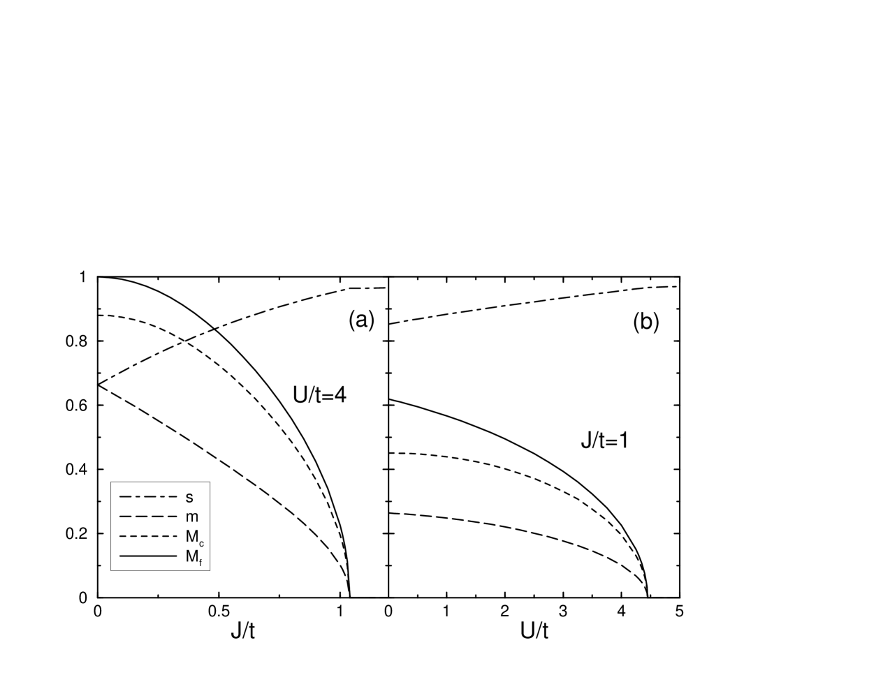
FIG. 1.: Mean-field order parameter $s$, $m$ and the staggered magnetizations $M_{c}$ and $M_{f}$ as function of (a) $J/t$ for $U/t=4$ and (b) $U/t$ for $J=t$.

Using (8) we may express the spectral function $A_{c}({\vec{k}},\omega)$ of the conduction electron $c_{\vec{k}}$ via a multi-particle correlation function of the $s$, $t$, $a$ and $b$ operators. On the mean-field level however, this simplifies into a linear combination of one-particle propagators of the $a$ and $b$ fermions only, involving both, diagonal as well as off-diagonal contributions. After some algebra we get

$$A_{c}({\vec{k}},z)=$$ (32)

$$-\frac{1}{\pi}{\rm Im}\frac{(m^{2}+s^{2})(z^{2}-\mu^{2})z+\epsilon_{\vec{k}}(z^{2}(s^{2}+m^{2})^{2}-4m^{2}s^{2}\mu^{2})}{\mu^{4}+4\epsilon_{\vec{k}}^{2}m^{2}\mu^{2}s^{2}-z^{2}(2\mu^{2}+\epsilon_{\vec{k}}^{2}(s^{2}+m^{2})^{2})+z^{4}}.$$ (33)

where $z=\omega+i\delta$.

III Results

A Magnetic phase diagram

FIG. 2.: Phase diagram of the Kondo-Hubbard model. Solid line: QMC, dot-dashed line: MF, dashed line: Spin Hamiltonian $H_{\rm spin}$ Eq. (34). Circles show parameter values, where the spectral function has been evaluated.

We start the discussion of our results with the magnetic phase diagram. At $U=0$ the UKLM maps onto the KLM. In the latter, the competition between the Ruderman-Kittel-Kasuya-Yosida (RKKY) interaction and the Kondo screening leads to a quantum phase transition between an ordered magnetic state and the disordered singlet phase at $J_{c}/t\sim 1.5$ [12, 4, 5]. For $U/t\rightarrow\infty$ double occupancy of the conduction electron sites is suppressed and the model maps onto a pure spin Hamiltonian of the form:

$$H_{\rm spin}=J_{\parallel}\sum_{\langle\vec{i},\vec{j}\rangle}\vec{S}^{c}_{\vec{i}}\vec{S}^{c}_{\vec{j}}+J\sum_{\vec{i}}\vec{S}^{c}_{\vec{i}}\vec{S}^{f}_{\vec{i}}$$ (34)

with $J_{\parallel}=4t^{2}/U$. Hence in the limit $U\rightarrow\infty$, $J_{c}$ vanishes and the ground state is a product of singlets on the $f$-$c$ bonds.

We have determined $J_{c}$ as a function of the Hubbard repulsion $U$ both, on the mean-field (MF) level and with the QMC method. Within MF theory the staggered magnetization is given by Eq. (31), while from the QMC method it is determined using the static spin-spin correlation function

$$S^{\alpha}\left(\vec{j}\right) = \left\langle\vec{S}_{\vec{j}}^{\alpha}\vec{S}_{0}^{\alpha}\right\rangle$$ (35)

$$S^{\alpha}\left(\vec{q}\right) = \sum_{\vec{j}}e^{i\vec{q}\vec{j}}S^{\alpha}\left(\vec{j}\right),$$ (36)

$\alpha=c(f)$ labels conduction(f) electron spins $S^{c(f)}_{\vec{j}}$ and the total spin $S^{tot}_{\vec{j}}$ is given by $S^{tot}_{\vec{j}}=S^{c}_{\vec{j}}+S^{f}_{\vec{j}}$. The staggered moment is extracted from finite size extrapolation

$$m^{\alpha}=\sqrt{\lim_{N\rightarrow\infty}S^{\alpha}\left(\vec{Q}\right)/N}$$ (37)

where $\vec{Q}=(\pi,\pi)$ and $N$ is the number of unit cells.

Fig. 2 depicts the phase diagram as a function of $J/t$ for finite $U/t$. The solid line refers to $QMC$ results, the dashed-dotted line shows the mean-field results. As anticipated already by the preceding discussion of the limiting points $U\rightarrow\infty$ and $U=0$, the critical value $J$ is a monotonically decreasing function of $U$. This can be understood as the Hubbard interaction tends to localize the conduction electrons leading to an effective reduction of the hopping amplitude. Hence, the formation of local singlets is favored. The above spin Hamiltonian (34) has been analyzed by Matsuhita and collaborators [13] who find a phase transition between a spin liquid and antiferromagnetically ordered phase at $(J_{\parallel}/J)_{c}=0.71$. This leads to $U_{c}=\frac{4t^{2}}{0.71J}$, the dashed line in fig. 2, in consistence with the results for the Kondo-Hubbard model in the large $U/t$ limit.

Finally Fig. 3 plots the staggered magnetization from a QMC scan at fixed $J$. The broken-symmetry ground state satisfies $m^{tot}=m^{f}-m^{c}$. In QMC $m^{tot}$ was calculated independently and up to $U\leq 4$ the above relation is fulfilled within the errorbars. With increasing $U$ conduction electrons get more and more localized and their local moment grows until it reaches the maximum of $\left\langle(\vec{S}_{\vec{j}}^{c})^{2}\right\rangle=3/4$ in the strong coupling region $U>8$. The staggered moments in the small $U\leq 4$ region are well understood within a Néel picture of almost fully ordered $f$-spins where the small local moment of a conduction electron is anti-parallel to the impurity spin. For larger values of $U$ dimerization becomes important which suppresses both $m^{c,f}$.

FIG. 3.: Staggered magnetization for a fixed $J=0.6$.

FIG. 4.: Single particle spectral function for pure Hubbard model at $U=4$, $U=6$ and $U=8$. For the QMC data (solid lines) we have normalized the maximum peak heights to unity. The numbers on the left-hand side of the figures correspond to the normalization factor. The vertical bars show the MF dispersion relation.

B Single particle spectral function.

To study the single-hole dynamics we analyze the spectral function $A(\vec{k},\omega)$, both using the MF expression (32) as well as results from the QMC. Within the QMC approach we first evaluate the imaginary time Greens function

$\displaystyle G_{\vec{k}}\left(\tau\right)=\frac{\left\langle\Psi_{0}\right|c_{\vec{k}}^{\dagger}\left(\tau\right)c_{\vec{k}}\left|\Psi_{0}\right\rangle}{\left\langle\Psi_{0}\right|\left.\Psi_{0}\right\rangle}=\frac{1}{\pi}\int_{0}^{\infty}d\omega e^{-\tau\omega}A\left(\vec{k},-\omega\right).$

from which $A(\vec{k},\omega)$ is extracted using the maximum entropy (ME) method [14].

We begin with the pure Hubbard model. In Fig. 4 we plot $A(\vec{k},\omega)$ as obtained from QMC as well as the MF dispersion as a function of $U/t$. While the comparison of the QMC with the MF dispersion is favorable one has to realize that the MF approach overestimates the quasiparticle gap. Therefore the MF band structure in these figures results from taking only $s$ and $m$ as obtained from the self-consistency equations (26) however adjusting $\mu$ such as to obtain the QMC gap at $\vec{k}=(\frac{\pi}{2},\frac{\pi}{2})$. At weak coupling $U/t\ll 1$ we find that the overall form of the low-energy dispersion is well reproduced by a functional form $\pm(\Delta^{2}+\epsilon(\vec{k})^{1/2}$ which is consistent with that in a spin density wave (SDW) state. Exactly this dispersion emerges also from the bond-operator MF theory at $J=0$ where $E_{1,\vec{k}}$ reduces to the SDW dispersion and the spectral weight of excitations with the dispersion $E_{2,\vec{k}}$ vanishes. For $J=0$ the condensate densities for the triplet and singlet are identical, i.e. $m=s$, which is equivalent to a Néel state of the $f$-spins.

At strong coupling $U/t\gg 1$ the Hubbard model maps approximately onto the $t$-$J_{\parallel}$ model with $J_{\parallel}=4t^{2}/U$. Monte Carlo results for the latter model at $J_{\parallel}/t<1$ show the existence of a quasiparticle band of width $\sim J_{\parallel}$ [15]. This should be compared to an identical spectral feature which can be observed in our QMC data for the Hubbard model upon enhancing $U/t$ in fig. 4b,c) (see also [16]). Especially along the line from $\vec{k}=(0,\pi)$ to $\vec{k}=(0,0)$, this narrow quasi particle band is clearly visible. In principle one should observe a similar band along $(0,\pi)$–$(\pi,\pi)$, however, due to small spectral weight in this region, we are unable to resolve this feature. Of particular importance is, that for the parameters we have investigated, the momenta of the dominant lowest energy hole-states for the Hubbard model are found on the boundary of the magnetic Brillouin zone. For the calculations presented in this work we have been unable to resolve an energy difference between the $(\pi/2,\pi/2)$ and $(0,\pi)$ points.

Next we turn to the UKLM at finite $J$. In fig. 5 we show a scan of QMC spectral functions and the MF dispersion ranging from the Kondo phase for $J/t=1.5$ and $U/t=4$ to the antiferromagnetic phase at $J/t=0.4,0.6$ and $U/t=4$. As for the pure Hubbard model the QMC and MF results are reasonably consistent. From the perturbative argument for $J/t>>1$, given in section I, we expect the momenta of the dominant lowest energy hole-states to occur at $\vec{k}=(\pm\pi,\pm\pi)$. As can be seen from fig. 5a) this is in consistent, both with the QMC as well as with the MF results. Moreover the QMC and MF dispersion agree very well.

FIG. 5.: Single particle spectra for the Kondo phase (a) and in the antiferromagnetic phase (b,c). Vertical bars show the MF dispersion.

Lowering $J$ as in fig. 5a)-c) reveals the evolution of the spectral density on going from the Kondo to the antiferromagnetically ordered phase. In fact, as $J$ approaches zero additional bands with a dispersion similar to the pure Hubbard case, i.e. 4a), develop. Yet, in the antiferromagnetically ordered phase, but for a finite $J$ the lowest energy hole-states are still Kondo-like, i.e. they occur at $\vec{k}=(\pm\pi,\pm\pi)$ as can be seen in fig. 5b),c). However, the weight of this excitation decreases continuously with decreasing $J$ and vanishes at $J=0$. The weight of the Hubbard-like band at $\vec{k}=(\pi,\pi)$ increases from zero in the spin singlet phase to its maximum value at $J=0$. Therefore we can interpret the change in the spectral function with decreasing $J$ as a continuous transfer of weight from Kondo-like to Hubbard-like bands. This shift of spectral weight renders the $J=0$ point singular since there is a sudden change of the wave vector which dominates the low energy hole dynamics.

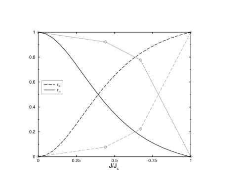
FIG. 6.: Relative spectral weight of Hubbard-band vs. Kondo-band. Thick lines: MF. Thin lines: QMC.

These findings are corroborated by our MF results. In fig. 6 the relative weight $r_{H(K)}=Z_{H(K)}/(Z_{H}+Z_{K})$ of the lower(upper) Hubbard(Kondo)-like band at momentum $\vec{k}=(\pi,\pi)$ as obtained from integrating $A_{c}(\vec{k},\omega)$ is depicted. In the QMC approach $Z_{K}$ results from fitting the long-time tail of the Greens function at $\vec{k}=(\pi,\pi)$ to the form $Z_{K}^{-\Delta_{qp}\tau}$ where $\Delta_{qp}$ corresponds to the quasiparticle gap. In turn $Z_{H}$ is obtained from the sum rule $Z_{K}+Z_{H}=\pi n(\vec{k})$ assuming a two-pole structure. Both, the QMC and the MF approximation display the same overall trend: at $J/t=0$ the total weight is in the Hubbard-like band while with increasing $J$ it becomes distributed into both bands. In the Kondo phase the Hubbard band disappears completely. In addition fig. 6 shows, that the MF approximation underestimates the spectral weight in the Hubbard-like band.

FIG. 7.: Mean-field spectral function Eq. 32 in the antiferromagnetic phase.

To compare the momentum dependence of the spectral weight as obtained from the MF theory with that of the QMC fig. 7 depicts $A_{c}(\vec{k},\omega)$ from (32) for $U/t=4$ and $J/t=0.4$. For visualization purpose, we have smeared the delta-function like MF-spectrum by a finite imaginary part $\delta=0.03$. The weight of these delta-peaks strongly varies as a function of $\vec{k}$ having its maximum around $(0,0)$ and a very small value in the vicinity of $(\pi,\pi)$. Again, this is consistent with the QMC data of fig. 5c). Obviously, since the imaginary part of the self energy vanishes in the MF approximation, the broadening of the QMC spectral function is not reproduced. Note however, that on the QMC side pinning down the details of the line shape is extremely challenging.

IV Conclusion

We have considered the single-hole dynamics in the Kondo-Hubbard model using both, QMC methods and a bond-operator mean-field approximation. Both approaches allow for similar conclusions. The UKLM shows a magnetic order-disorder transition. At $U=0$ this transition is triggered by the competition between the RKKY interaction and the Kondo screening and occurs at $J_{c}/t\sim 1.5$. In the large $U/t$ limit the model maps onto a bilayer spin-model and $J_{c}$ scales to zero. Our results show that both limiting cases are linked continuously and that $J_{c}$ is a monotonically decreasing function of $U$. Hence as far as $J_{c}$ is concerned the dominant effect of the Hubbard interaction $U$ is to localize the conduction electrons which favors screening of the localized spins.

The single particle spectral function was shown to be insensitive to the magnetic phase transition. Irrespective of $U$ and $J>0$ the dominant low energy hole-states are found at the momenta $\vec{k}=(\pm\pi,\pm\pi)$. These excitations originate from the screening of the magnetic impurities and hence are local. In the ordered phase pronounced shadow features can be observed. As $J\rightarrow 0$, the spectral weight in the Kondo-like low energy band in the vicinity of $\vec{k}=(\pm\pi,\pm\pi)$ vanishes and is transfered to higher energy Hubbard-like bands. In the $(U,J)$-plane the Hubbard-line, i.e. $J=0$, is singular since the localized spins decouple and lead to a macroscopically degenerate ground state. In turn, the evolution of the spectral function is discontinuous in as such that at $J=0$ there is a sudden change of the wave vector which dominates the low energy hole dynamics. In this sense the model shows no continuous path from the Kondo insulator to the Mott insulator.

The singularity of the UKLM at $J=0$ may be alleviated by including an antiferromagnetic coupling between the localized $f$-spins. In the large $U/t$ limit this leads to a bilayer spin model which has been considered by Vojta and Becker [17]. The authors arrive at a similar conclusion namely that hole dynamics are governed by local spin environment. Numerical work on this modified model is presently under progress.

Given our results it is very tempting to speculate on the effects of doping with a finite density of holes $n_{h}$ away from half filling. In the limit $J/t\rightarrow\infty$ the Kondo lattice model can be mapped onto a Hubbard model with a Coulomb repulsion $\tilde{u}\rightarrow\infty$ and a particle density $n_{h}$ [18]. In this low-density limit single particle renormalizations [19] may be neglected which suggests that doping the UKLM can be understood approximately within a rigid-band picture. From this we would conclude that off half filling the UKLM displays a Fermi surface centered around $\vec{k}=(\pm\pi,\pm\pi)$ for all values of $U$ and $J>0$.

REFERENCES

- [1] W. F. Brinkman and T. M. Rice, Phys. Rev. B 2, 1324 (1970).
- [2] M. Imada, A. Fujimori, and Y. Tokura, Rev. Mod. Phys. 70, 1039 (1998).
- [3] H. Tsunetsugu, M. Sigrist, and K. Ueda, Rev. Mod. Phys. 69, 809 (1997).
- [4] F. F. Assaad, Phys. Rev. Lett. 83, 796 (1999).
- [5] S. Capponi and F. F. Assaad, Phs. Rev. B 63, 155113 (2001).
- [6] M. Feldbacher and F. F. Assaad, Phys. Rev. B 63, 73105 (2001).
- [7] C. Jurecka and W. Brenig, cond-mat/0103511 .
- [8] S. Sachdev and R. N. Bhatt, Phys. Rev. B 41, 9323 (1990).
- [9] R. Eder, Y. Ohta, and G. A. Sawatzky, Phys. Rev. B 55, 3414 (1997).
- [10] R. Eder, O. Rogojanu, and G. A. Sawatzky, Phys. Rev. B 58, 7599 (1998).
- [11] B. Normand and T. Rice, Phys. Rev. B 56, 8760 (1997).
- [12] S. Doniach, Physica B 91, 231 (1977).
- [13] Y. Matsushita, M. P. Gelfand, and C. Ishii, J. Phs. Soc. Jpn. 66, 1153 (1997).
- [14] M. Jarrell and J. Gubernatis, Physics Reports 269, 133 (1996).
- [15] M. Brunner, F. F. Assaad, and A. Muramatsu, Phys. Rev. B 62, 12395 (2000).
- [16] R. Preuss, W. Hanke, and W. von der Linden, Phys. Rev. Lett. 75, 1344 (1995).
- [17] M. Vojta and K. W. Becker, Phys. Rev. B 60, 15201 (1999).
- [18] C. Lacroix, Solid Stat. Commun. 54, 991 (1985).
- [19] A. L. Fetter and J. Walecka, Quantum theory of many-particle systems (McGraw-Hill, New-York, 1971).