Thermodynamic Formalism of the Harmonic Measure of Diffusion Limited Aggregates: Phase Transition and Converged $f(\alpha)$

Abstract

We study the nature of the phase transition in the multifractal formalism of the harmonic measure of Diffusion Limited Aggregates (DLA). Contrary to previous work that relied on random walk simulations or ad-hoc models to estimate the low probability events of deep fjord penetration, we employ the method of iterated conformal maps to obtain an accurate computation of the probability of the rarest events. We resolve probabilities as small as $10^{-70}$. We show that the generalized dimensions $D_{q}$ are infinite for $q<q^{*}$, where $q^{*}=-0.17\pm 0.02$. In the language of $f(\alpha)$ this means that $\alpha_{\rm max}$ is finite. We present a converged $f(\alpha)$ curve.

Since its introduction in 1981 [1] the model of Diffusion Limited Aggregation (DLA) has posed a challenge to our understanding of fractal and multifractal phenomena. DLA is a paradigmatic example for the spontaneous generation of fractal objects by simple dynamical rules (being generated by random walkers); its harmonic measure, which is the probability for a random walker to hit the surface, had been one of the first studied examples of multifractal measures outside the realm of ergodic measures in dynamical systems [2]. The multifractal properties stem from the extreme contrast between the probability to hit the tips of the DLA compared with penetrating the fjords.

The multifractal properties of the harmonic measure of the DLA are conveniently studied in the context of the generalized dimensions $D_{q}$, and the associated $f(\alpha)$ function [3, 4]. The simplest definition of the generalized dimensions is in terms of a uniform covering of the boundary of a DLA cluster with boxes of size $\ell$, and measuring the probability for a random walker coming from infinity to hit a piece of boundary which belongs to the $i$’th box. Denoting this probability by $P_{i}(\ell)$, one considers [3]

$$D_{q}\equiv\lim_{\ell\to 0}\frac{1}{q-1}\frac{\log\sum_{i}P_{i}^{q}(\ell)}{\log\ell}\ .$$ (1)

It is well known by now that the existence of an interesting spectrum of values $D_{q}$ is related to the probabilities $P_{i}(\ell)$ having a spectrum of “singularities” in the sense that $P_{i}(\ell)\sim\ell^{\alpha}$ with $\alpha$ taking on values from a range $\alpha_{\rm min}\leq\alpha\leq\alpha_{\rm max}$. The frequency of observation of a particular value of $\alpha$ is determined by the the function $f(\alpha)$ where (with $\tau(q)\equiv(q-1)D_{q}$)

$$f(\alpha)=\alpha q(\alpha)-\tau\Big{(}q\left(\alpha\right)\Big{)}\ ,\quad\frac{\partial\tau(q)}{\partial q}=\alpha(q)\ .$$ (2)

The understanding of the multifractal properties and the associated $f(\alpha)$ spectrum of DLA clusters have been a long standing issue. Of particular interest are the values of the minimal and maximal values, $\alpha_{min}$ and $\alpha_{max}$, relating to the largest and smallest growth probabilities, respectively. As a DLA cluster grows the large branches screen the deep fjords more and more and the probability for a random walker to get into these fjords (say around the seed of the cluster) becomes smaller and smaller. A small growth probability corresponds to a large value of $\alpha$. Previous literature hardly agrees about the actual value of $\alpha_{max}$. Ensemble averages of the harmonic measure of DLA clusters indicated a rather large value of $\alpha_{max}\sim 8$ [5]. In subsequent experiments on non-Newtonian fluids [6] and on viscous fingers [7], similar large values of $\alpha_{max}$ were also observed. These numerical and experimental indications of a very large value of $\alpha_{max}$ led to a conjecture that, in the limit of a large, self-similar cluster some fjords will be exponentially screened and thus causing $\alpha_{max}\to\infty$ [8].

If indeed $\alpha_{max}\to\infty$, this can be interpreted as a phase transition [9] (non-analyticity) in the $q$ dependence of $D_{q}$, at a value of $q$ satisfying $q\geq 0$. If the transition takes place for a value $q<0$ then $\alpha_{max}$ is finite. Lee and Stanley [10] proposed that $\alpha_{max}$ diverges like $R^{2}/\ln{R}$ with $R$ being the radius of the cluster. Schwarzer et al. [11] proposed that $\alpha_{max}$ diverges only logarithmically in the number of added particles. Blumenfeld and Aharony [12] proposed that channel-shaped fjords are important and proposed that $\alpha_{max}\sim{{M^{x}}\over{ln~{}M}}$ where $M$ is the mass of the cluster; Harris and Cohen [13], on the other hand, argued that straight channels might be so rare that they do not make a noticeable contribution, and $\alpha_{max}$ is finite, in agreement with Ball and Blumenfeld who proposed [14] that $\alpha_{max}$ is bounded below 11. Obviously, the issue was not quite settled. The difficulty is that it is very hard to estimate the smallest growth probabilities using models or direct numerical simulations.

In this Letter we use the method of iterated conformal maps to offer an accurate determination of the probability for the rarest events. We propose that using this method we can settle the issue in a conclusive way. Our result is that $\alpha_{max}$ exists and the phase transition occurs at a $q$ value that is slightly negative. In this method one studies DLA by constructing $\Phi^{(n)}(w)$ which conformally maps the exterior of the unit circle $e^{i\theta}$ in the mathematical $w$–plane onto the complement of the (simply-connected) cluster of $n$ particles in the physical $z$–plane [15, 16, 17]. The unit circle is mapped onto the boundary of the cluster. The map $\Phi^{(n)}(w)$ is made from compositions of elementary maps $\phi_{\lambda,\theta}$,

$$\Phi^{(n)}(w)=\Phi^{(n-1)}(\phi_{\lambda_{n},\theta_{n}}(w))\ ,$$ (3)

where the elementary map $\phi_{\lambda,\theta}$ transforms the unit circle to a circle with a semi-circular “bump” of linear size $\sqrt{\lambda}$ around the point $w=e^{i\theta}$. We use below the same map $\phi_{\lambda,\theta}$ that was employed in [15, 16, 17, 18, 19]. With this map $\Phi^{(n)}(w)$ adds on a semi-circular new bump to the image of the unit circle under $\Phi^{(n-1)}(w)$. The bumps in the $z$-plane simulate the accreted particles in the physical space formulation of the growth process. Since we want to have fixed size bumps in the physical space, say of fixed area $\lambda_{0}$, we choose in the $n$th step

$$\lambda_{n}=\frac{\lambda_{0}}{|{\Phi^{(n-1)}}^{\prime}(e^{i\theta_{n}})|^{2}}\ .$$ (4)

The recursive dynamics can be represented as iterations of the map $\phi_{\lambda_{n},\theta_{n}}(w)$,

$$\Phi^{(n)}(w)=\phi_{\lambda_{1},\theta_{1}}\circ\phi_{\lambda_{2},\theta_{2}}\circ\dots\circ\phi_{\lambda_{n},\theta_{n}}(\omega)\ .$$ (5)

It had been demonstrated before that this method represents DLA accurately, providing many analytic insights that are not available otherwise [18, 19]. For our purposes here we quote a result established in [16], which is

$$\langle\lambda^{q}_{n}\rangle\equiv(1/2\pi)\int_{0}^{2\pi}\lambda^{q}_{n}(\theta)d\theta\sim n^{-2qD_{2q+1}/D}\ .$$ (6)

To compute $\tau(q)$ we rewrite this average as

$$\langle\lambda^{q}_{n}\rangle=\int ds\left|\frac{d\theta}{ds}\right|~{}\lambda^{q}_{n}(s)=\int ds\frac{\lambda^{q+1/2}(s)}{\sqrt{\lambda_{0}}}\ ,$$ (7)

where $s$ is the arc-length of the physical boundary of the cluster. In the last equality we used the fact that $|d\theta/ds|=\sqrt{\lambda_{n}/\lambda_{0}}$. We stress at this point that in order to measure these moments for $q\leq 0$ we must go into arc-length representation.

To make this crucial point clear we discuss briefly what happens if one attempts to compute the moments from the definition (6). Having at hand the conformal map $\Phi^{(n)}(e^{i\theta})$, one can choose randomly as many points on the unit circle $[0,2\pi]$ as one wishes, obtain as many (accurate) values of $\lambda_{n}$, and try to compute the integral as a finite sum. The problem is of course that using such an approach the fjords are not resolved. To see this we show in Fig.1 panel a the region of a typical cluster of 50 000 particles that is being visited by a random search on the unit circle. Like in direct simulations using random walks, the rarest events are not probed, and no serious conclusion regarding the phase transition is possible.

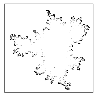
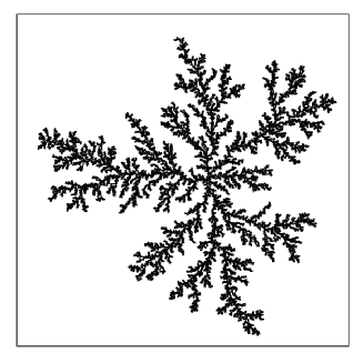
FIG. 1.: panel a: the boundary of the cluster probed by a random search with respect to the harmonic measure. Panel b: the boundary of the cluster probed by the present method.

Another method that cannot work is to try to compute by sampling on the arc-length in a naive way. The reason is that the inverse map $[\Phi^{(n)}]^{-1}(s)$ cannot resolve $\theta$ values that belong to deep fjords. As the growth proceeds, reparametrization squeezes the $\theta$ values that map to fjords into minute intervals, below the computer numerical resolution. To compute the values of $\lambda_{n}(s)$ effectively we must use the full power of our iterated conformal dynamics, carrying the history with us, to iterate forward and backward at will to resolve accurately the $\theta$, $\lambda$ values of any given particle on the fully grown cluster.

To do this we recognize that every time we grow a semi-circular bump we generate two new branch-cuts in the map $\Phi^{(n)}$. We find the position on the boundary between every two branch-cuts, and there compute the value of $\lambda_{n}$. The first step in our algorithm is to generate the location of these points intermediate to the branch-cuts [20]. Each branch-cut has a preimage on the unit circle which will be indexed with 3 indices, $w^{k(\ell)}_{j,\ell}\equiv\exp[i\theta^{k(\ell)}_{j,\ell}]$. The index $j$ represents the generation when the branch-cut was created (i.e. when the $j$th particle was grown). The index $\ell$ stands for the generation at which the analysis is being done (i.e. when the cluster has $\ell$ particles). The index $k$ represents the position of the branch-cut along the arc-length, and it is a function of the generation $\ell$. Note that since bumps may overlap during growth, branch-cuts are then covered, and therefore the maximal $k$, $k_{max}\leq 2\ell$. After each iteration the preimage of each branch-cut moves on the unit circle, but its physical position remains. This leads to the equation that relates the indices of a still exposed branch-cut that was created at generation $j$ to a later generation $n$:

$$\Phi^{(n)}(w^{k(n)}_{j,n}) \equiv \Phi^{(n)}\left(\phi^{-1}_{\lambda_{n},\theta_{n}}\circ\dots\circ\phi^{-1}_{\lambda_{j+1},\theta_{j+1}}(w^{\tilde{k}(j)}_{j,j})\right)$$ (8)

$$= \Phi^{(j)}(w^{\tilde{k}(j)}_{j,j})\ .$$ (9)

Note that the sorting indices $\tilde{k}(j)$ are not simply related to $k(n)$, and needs to be tracked as follows. Suppose that the list $w^{k(n-1)}_{j,n-1}$ is available. In the $n$th generation we choose randomly a new $\theta_{n}$, and find two new branch-cuts which on the unit circle are at angles $\theta_{n}^{\pm}$. If one (or very rarely more) branch-cut of the updated list $\phi^{-1}_{\lambda_{n},\theta_{n}}(w^{k(n-1)}_{j,n-1})$ is covered, it is eliminated from the list, and together with the sorted new pair we make the list $w^{k(n)}_{j,n}$. Having a cluster of $n$ particles we now consider all neighboring pairs of preimages $w^{k(n)}_{j,n}$ and $w^{k(n)+1}_{J,n}$, that very well may have been created at two different generations $j$ and $J$. The larger of these indices ($J$ without loss of generality) determines the generation of the intermediate position at which we want to compute the field. We want to find the preimage $u^{k(n)}_{J,J}$ of this mid-point on the unit circle , to compute $\lambda_{k(n)}$ there accurately. Using definition (9) we find the preimage

$$\arg(u^{k(n)}_{J,J})=[\arg(w^{\tilde{k}(J)}_{j,J})+\arg(w^{\tilde{k}(J)+1}_{J,J})]/2\ .$$ (10)

In Fig.1 panel b we show, for the same cluster of 50 000, the map $\Phi^{(J)}(u^{k(n)}_{J,J})$ with $k(n)$ running between 1 and $k_{\rm max}$, with $J$ being the corresponding generation of creation of the mid point. We see that now all the particles are probed, and every single value of $\lambda_{k(n)}$ can be computed. However, to compute these $\lambda_{k(n)}$ accurately, we define (in analogy to Eq.(9)) for every $J<m\leq n$

$$u^{k(n)}_{J,m}\equiv\phi^{-1}_{\lambda_{m},\theta_{m}}\circ\dots\circ\phi^{-1}_{\lambda_{j+1},\theta_{j+1}}(u^{k(n)}_{J,J})\ .$$ (11)

Finally $\lambda_{k(n)}$ is computed from the definition (4) with

$${\Phi^{(n)}}^{\prime}(u^{k(n)}_{J,n}) = \phi^{\prime}_{\lambda_{n},\theta_{n}}(u^{k(n)}_{J,n})\cdots\phi^{\prime}_{\lambda_{J+1},\theta_{J+1}}(u^{k(n)}_{J,J+1})$$ (12)

$$\times {\Phi^{(J)}}^{\prime}(u^{k(n)}_{J,J})\ .$$ (13)

This calculation is optimally accurate since we avoid as much as possible the effects of the exponential shrinking of low probability regions on the unit circle. Each derivative in (13) is computed using information from a generation in which points on the unit circle are optimally resolved.

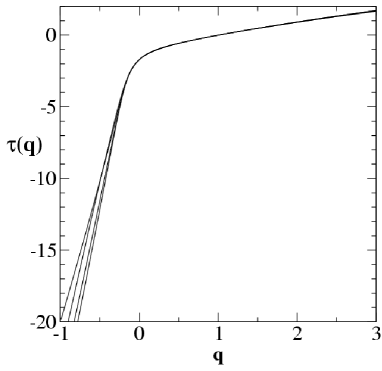
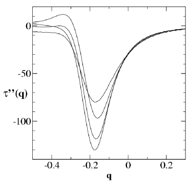
FIG. 2.: Panel a: the calculated function $\tau(q)$ for clusters of $n$ particles, with $n=$10 000,15 000, 25 000 and 30 000. Panel b: the second derivative of $\tau(q)$ with respect to $q$.

The integral (7) is then estimated as the finite sum $\sqrt{\lambda_{0}}\sum_{k(n)}\lambda_{k(n)}^{q}$. We should stress that for clusters of the order of 30 000 particles we already compute, using this algorithm, $\lambda_{k(n)}$ values of the order of $10^{-70}$. To find the equivalent small probabilities using random walks would require about $10^{70}$ attempts to see them just once. This is of course impossible, explaining the lasting confusion about the issue of the phase transition in this problem. This also means that all the $f(\alpha)$ curves that were computed before [5, 21] did not converge. Note that in our calculation the small values of $\lambda_{k(n)}$ are obtained from multiplications rather than additions, and therefore can be trusted.

Having the accurate values $\lambda_{k(n)}$ we can now compute the moments (6). Since the scaling form on the RHS includes unknown coefficients, we compute the values of $\tau(q)$ by dividing $\langle\lambda_{n}^{q}\rangle$ by $\langle\lambda_{\bar{n}}^{q}\rangle$, estimating

$$\tau(q)\approx-D\frac{\log{\langle\lambda_{n}^{q}\rangle}-\log{\langle\lambda_{\bar{n}}^{q}\rangle}}{\log{n}-\log{\bar{n}}}$$ (14)

Results for $\tau(q)$ for increasing values of $n$ and $\bar{n}$ are shown in Fig. 2, panel (a). It is seen that the value of $\tau(q)$ appears to grow without bound for $q$ negative. The existence of a phase transition is however best indicated by measuring the derivatives of $\tau(q)$ with respect to $q$. In Fig. 2 panel b we show the second derivative, indicating a phase transition at a value of $q$ that recedes away from $q=0$ when $n$ increases. Due to the great accuracy of our measurement of $\lambda$ we can estimate already with clusters as small as 20-30 000 the $q$ value of the phase transition to $q=-0.17\pm 0.02$. The fact that this value is very close to the converged value can be seen from the $f(\alpha)$ curve which is plotted in Fig. 3. A test of convergence is that the slope of this function where it becomes essentially linear must agree with the $q$ value of the phase transition. The straight line shown in Fig.3 has the slope of -0.17, and it indeed approximates very accurately the slope of the $f(\alpha)$ curve where it ends and stops being analytic. The reader should also note that the peak of the curve agrees with $D\approx 1.71$, as well as the fact that $\tau(3)$ is also $D$ as expected in this problem. The value of $\alpha_{\rm max}$ is close to 20, which is higher than anything predicted before. It is nevertheless finite. We believe that this function is well converged, in contradistinction with past calculations.

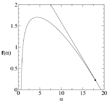
FIG. 3.: The calculated function $f(\alpha)$ using $\tau(q)$ calculated from a cluster with $n=30~{}000$ particles. This $f(\alpha)$ is almost indistinguishable from the one computed with $n=25000$ particles. We propose that this function is well converged. The black dot denotes where the curve ends, being tangent to the line with slope -0.17.

REFERENCES

- [1] T.A. Witten and L. Sander, Phys. Rev. Lett. 47, 1400 (1981).
- [2] T.C. Halsey, P. Meakin and I. Procaccia, Phys. Rev. Lett. 56, 854 (1986).
- [3] H.G.E. Hentschel and I. Procaccia, Physica D8, 435 (1983).
- [4] T.C. Halsey, M.H. Jensen, L.P. Kadanoff, I. Procaccia and B. Shraiman, Phys. Rev. A 33, 1141 (1986).
- [5] C. Amitrano, A. Coniglio and F. di Liberto, Phys.Rev.Lett. 57, 1098 (1986).
- [6] J. Nittmann, H.E. Stanley, E. Touboul and G. Daccord, Phys.Rev.Lett. 58, 619 (1987).
- [7] K.J. Måløy, F. Boger, J. Feder, and T. Jøssang, in “Time-Dependent Effects in Disordered Materials”, eds. R. Pynn and T. Riste, (Plenum, New York, 1987), p.111.
- [8] T. Bohr, P. Cvitanović and M.H. Jensen, Europhys.Lett. 6, 445 (1988).
- [9] P. Cvitanović, in Proceedings of “XIV Colloquium on Group Theoretical Methods in Physics”, ed. R.Gilmore (World Scientific, Singapore 1987); in “Non-Linear Evolution and Chaotic Phenomena”, eds. P. Zweifel, G. Gallavotti and M. Anile (Plenum, New York, 1988).
- [10] J. Lee and H.E. Stanley, Phys.Rev.Lett. 61, 2945 (1988).
- [11] S. Schwarzer, J. Lee, A. Bunde, S. Havlin, H.E. Roman and H.E. Stanley, Phys.Rev. Lett. 65, 603 (1990).
- [12] R. Blumenfeld and A. Aharony, Phys.Rev.Lett. 62, 2977 (1989)
- [13] A.B. Harris and M. Cohen, Phys.Rev.A 41, 971 (1990).
- [14] R.C. Ball and R. Blumenfeld, Phys. Rev. A 44, R828, (1991).
- [15] M.B. Hastings and L.S. Levitov, Physica D 116, 244 (1998).
- [16] B. Davidovitch, H.G.E. Hentschel, Z. Olami, I.Procaccia, L.M. Sander, and E. Somfai, Phys. Rev. E, 59 1368 (1999).
- [17] B. Davidovitch, M.J. Feigenbaum, H.G.E. Hentschel and I. Procaccia, Phys. Rev. E 62, 1706 (2000).
- [18] B. Davidovitch and I. Procaccia, Phys. Rev. Lett., 85 3608-3611 (2000).
- [19] B. Davidovitch, A. Levermann, I. Procaccia, Phys. Rev. E, 62 R5919.
- [20] F. Barra, B. Davidovitch and I. Procaccia, “Iterated Conformal Dynacmics and Laplacian Growth”, submitted to Phys.Rev. E, also cond-mat/0105608.
- [21] Y. Hayakawa, S. Sato and M. Matushita, Phys. Rev. A 36, 1963 (1987).