Complex-Temperature Phase Diagrams for the $q$-State Potts Model on Self-Dual Families of Graphs and the Nature of the $q\to\infty$ Limit

Shu-Chiuan Chang and Robert Shrock

C. N. Yang Institute for Theoretical Physics

State University of New York

Stony Brook, NY 11794-3840

We present exact calculations of the Potts model partition function $Z(G,q,v)$ for arbitrary $q$ and temperature-like variable $v$ on self-dual strip graphs $G$ of the square lattice with fixed width $L_{y}$ and arbitrarily great length $L_{x}$ with two types of boundary conditions. Letting $L_{x}\to\infty$, we compute the resultant free energy and complex-temperature phase diagram, including the locus ${\cal B}$ where the free energy is nonanalytic. Results are analyzed for widths $L_{y}=1,2,3$. We use these results to study the approach to the large-$q$ limit of ${\cal B}$.

I Introduction

The $q$-state Potts model has served as a valuable model for the study of phase transitions and critical phenomena [1, 2]. On a lattice, or, more generally, on a (connected) graph $G$, at temperature $T$, this model is defined by the partition function

$$Z(G,q,v)=\sum_{\{\sigma_{n}\}}e^{-\beta{\cal H}}$$ (1)

with the (zero-field) Hamiltonian

$${\cal H}=-J\sum_{\langle ij\rangle}\delta_{\sigma_{i}\sigma_{j}}$$ (2)

where $\sigma_{i}=1,...,q$ are the spin variables on each vertex $i\in G$; $\beta=(k_{B}T)^{-1}$; and $\langle ij\rangle$ denotes pairs of adjacent vertices. The graph $G=G(V,E)$ is defined by its vertex set $V$ and its edge (bond) set $E$; we denote the number of vertices of $G$ as $n=n(G)=|V|$ and the number of edges of $G$ as $e(G)=|E|$. We use the notation

$$K=\beta J\ ,\quad a=e^{K}=u^{-1}\ ,\quad v=a-1$$ (3)

so that the physical ranges are (i) $a\geq 1$, i.e., $v\geq 0$ corresponding to $\infty\geq T\geq 0$ for the Potts ferromagnet (FM), with $J>0$, and (ii) $0\leq a\leq 1$, i.e., $-1\leq v\leq 0$, corresponding to $0\leq T\leq\infty$ for the Potts antiferromagnet (AFM), with $J<0$. One defines the (reduced) free energy per site $f=-\beta F$, where $F$ is the actual free energy, via

$$f(\{G\},q,v)=\lim_{n\to\infty}\ln[Z(G,q,v)^{1/n}]$$ (4)

where we use the symbol $\{G\}$ to denote $\lim_{n\to\infty}G$ for a given family of graphs.

On a two-dimensional lattice, for the $q=2$ Ising case, and for $q=3,4$, the Potts ferromagnet exhibits a second-order phase transition from a paramagnetic (PM) high-temperature phase to a low-temperature phase with spontaneously broken symmetry and long-range ferromagnetic order (magnetization). For $q>4$, this transition is first-order, with a latent heat that increases monotonically with $q$, approaching a limiting constant as $q\to\infty$ [2, 3]. The behavior of the Potts antiferromagnet depends on the value of $q$ and the type of lattice, as will be discussed further below.

Let $G^{\prime}=(V,E^{\prime})$ be a spanning subgraph of $G$, i.e. a subgraph having the same vertex set $V$ and a subset of the edge set, $E^{\prime}\subseteq E$. Then $Z(G,q,v)$ can be written as the sum [4]

$$Z(G,q,v)=\sum_{G^{\prime}\subseteq G}q^{k(G^{\prime})}v^{e(G^{\prime})}$$ (5)

where $k(G^{\prime})$ denotes the number of connected components of $G^{\prime}$. Since we only consider connected graphs $G$, we have $k(G)=1$. The formula (5) enables one to generalize $q$ from ${\mathbb{Z}}_{+}$ to ${\mathbb{R}}_{+}$ (keeping $v$ in its physical range). The formula (5) shows that $Z(G,q,v)$ is a polynomial in $q$ and $v$ (equivalently, $a$). The Potts model partition function on a graph $G$ is essentially equivalent to the Tutte polynomial [5]-[7] and Whitney rank polynomial [2], [8]-[10] for this graph, and this connection will be useful below.

Using the formula (5) for $Z(G,q,v)$, one can generalize $q$ from ${\mathbb{Z}}_{+}$ not just to ${\mathbb{R}}_{+}$ but to ${\mathbb{C}}$ and $v$ from its physical ferromagnetic and antiferromagnetic ranges $0\leq v\leq\infty$ and $-1\leq v\leq 0$ to $v\in{\mathbb{C}}$. A subset of the zeros of $Z$ in the two-complex dimensional space ${\mathbb{C}}^{2}$ defined by the pair of variables $(q,v)$ form an accumulation set in the $n\to\infty$ limit, denoted ${\cal B}$, which is the continuous locus of points where the free energy is nonanalytic. The program of studying statistical mechanical models with external field generalized from ${\mathbb{R}}$ to ${\mathbb{C}}$ was pioneered by Yang and Lee [11], and the corresponding generalization of the temperature from physical to complex values was initiated by Fisher [12]. Here we allow both $q$ and the temperature-like variable $v$ to be complex. For a given value of $v$, one can consider this locus in the $q$ plane, and we shall sometimes denote it as ${\cal B}_{q}$, and similarly, for a given value of $q$ (not necessarily $\in{\mathbb{Z}}_{+}$), one can consider this locus in the plane of a complex-temperature variable such as $v$ or

$$\zeta=\frac{v}{\sqrt{q}}\ .$$ (6)

It will be convenient to introduce polar coordinates, letting $\zeta=|\zeta|e^{i\theta}$.

In this paper we shall present exact calculations of the Potts model partition function $Z(G,q,v)$ for arbitrary $q$ and $v$ on self-dual strip graphs $G$ of the square lattice with fixed width $L_{y}$ and arbitrarily great length $L_{x}$ with two types of boundary conditions. Letting $L_{x}\to\infty$, we compute the resultant free energy and complex-temperature phase diagram. Results are analyzed for widths $L_{y}=1,2,3$. We shall use these results to study the approach to the large-$q$ limit of ${\cal B}$.

There are several motivations for this study. Clearly, new exact calculations of Potts model partition functions on lattice strips with arbitrarily large numbers of vertices are of value in their own right. This is especially the case since the free energy of the Potts model has never been calculated exactly for $d\geq 2$ except in the $q=2$ Ising case in 2D. Just as the study of functions of a complex variable can yield a deeper understanding of functions of a real variable, so also the investigation of complex-temperature phase diagrams of spin models can provide further understanding of the physical behavior of these models. Besides [12], complex-temperature singularities were noticed in early series analyses (e.g., [13]), and many studies have been carried out on complex-temperature (Fisher) zeros of the partition function of the Ising model and its generalization to the $q$-state Potts model [14]-[61]. In particular, several exact determinations of complex-temperature phase diagrams of the Potts model on infinite-length, finite-width lattice strips [41, 52, 53, 54, 56, 57, 58], in comparison with both exact solutions for the $q=2$ 2D complex-temperature phase diagrams [12, 33, 37] and finite-lattice calculations of Fisher zeros [29, 38, 39, 43, 47, 48] have shown that, although the physical thermodynamic properties of these strips are essentially one-dimensional, one can nevertheless gain important insights into certain complex-temperature properties of the model on the corresponding two-dimensional lattice. For a model above its lower critical dimensionality, a complex-temperature phase diagram includes the complex-temperature extensions of the paramagnetic and ferromagnetic phases as well as a possible antiferromagnetic phase and other phases (denoted O in [33]) that have no overlap with any physical phase. For the infinite-length finite-width strips under consideration here, for finite $q$, the complex-temperature phase diagram includes only PM and O phases since there are no broken-symmetry phases.

An early study of the complex-temperature phase diagram for the square-lattice Potts model led to the suggestion that the locus ${\cal B}$, which is comprised of the circles $|a\pm 1|=\sqrt{2}$ for $q=2$ [12] might generalize to the union of the circles $|a-1|=\sqrt{q}$ and $|a+1|=\sqrt{4-q}$ for $1\leq q\leq 4$ [22], but subsequent studies found that many of the Fisher zeros in the $Re(a)<0$ half-plane do not lie on a circular arc but instead show considerable scatter [23, 29, 38, 43]. The infinite square lattice is self-dual, and for calculations on finite sections of the square lattice, it was found to be useful to employ boundary conditions that preserve this self-duality. Stated more abstractly, one studies lattice graphs $G$ with the property that the planar dual, $G^{*}$, is isomorphic to $G$, which we write simply as $G=G^{*}$. Here we recall that the dual of a planar graph $G$ with $n$ vertices, $e$ edges, and $f$ faces is the graph $G^{*}$ obtained by associating a vertex of $G^{*}$ with each face of $G$ and connecting each pair of vertices on $G^{*}$ by edges running through the edges of $G$. It follows that $n(G^{*})=f(G)$, $e(G^{*})=e(G)$, and $f(G^{*})=n(G)$. The Potts model partition function satisfies the relation

$$Z(G,q,v)=q^{1-f(G)}v^{e(G)}Z(G^{*},q,v_{d})$$ (7)

where the dual image of $v$ is $v_{d}$, given by

$$v_{d}=\frac{q}{v}$$ (8)

i.e., in terms of $\zeta$, the duality map is the inversion map:

$$\zeta_{d}=\frac{1}{\zeta}\ .$$ (9)

Thus, it is also useful to plot Fisher zeros in terms of the variable $\zeta$, since the accumulation set ${\cal B}$ is invariant under inversion for a self-dual graph:

$$G=G^{*}\Longrightarrow{\cal B}\quad{\rm is\ invariant\ under}\quad\zeta\to\frac{1}{\zeta}\ .$$ (10)

It was found that complex-temperature zeros calculated for finite sections of the square with duality-preserving boundary conditions (DBC’s) have the appealing property of lying exactly on an arc of the unit circle $|\zeta|=1$ in the $\zeta$ plane for $Re(\zeta)\mathrel{\raisebox{-2.58334pt}{$\stackrel{{\scriptstyle\textstyle>}}{{\sim}}$}}0$ [29, 38, 39]. (For physical temperature the coefficients of powers of $a=e^{K}$ are positive, so there are no zeros on the positive real axis $Re(a)>0$ for any finite lattice. However, in the thermodynamic limit, the phase boundary crosses this axis at $a_{c}=1+\sqrt{q}$, i.e. $\zeta_{c}=1$.) In [43] several types of different self-dual boundary conditions were used in order to ascertain which features are common to each of these and hence might be relevant for the thermodynamic limit. However, because of the scatter of zeros in the $Re(a)<0$ half-plane and the dependence of the pattern of zeros, it has not so far been possible to reach a conclusion concerning the portion of the complex-temperature phase boundary ${\cal B}$ in this region (although some points on the boundary have been reliably located by analysis of series expansions [43]).

An interesting exact result was obtained by Wu and collaborators, who gave an elegant proof [39], using Euler’s identity for partitions, that for the Potts model on the square lattice, after having taken the thermodynamic limit so that zeros of $Z$ in the complex $\zeta$ plane have merged to form the continuous locus ${\cal B}$, if one takes the further limit $q\to\infty$, this locus ${\cal B}$ is the circle $|\zeta|=1$ for the square lattice. It is straightforward to show that the same conclusion holds if one keeps $L_{y}$ fixed and finite, and takes $L_{x}\to\infty$, after which one takes the limit $q\to\infty$. Thus, for the infinite-length limit of the self-dual strips that we consider here, $\lim_{q\to\infty}{\cal B}$ is again the unit circle $|\zeta|=1$. In 2D, the interior and exterior of this circle $|\zeta|=1$ form the complex-temperature extensions of the PM and FM phases, respectively. Since the infinite-length, finite-width strips under study here are quasi-one-dimensional systems, there cannot be any broken-symmetry phase at finite temperature for a spin model with short-range interactions and hence there is no FM phase or its complex-temperature extension. Note that any finite temperature point, i.e. $-1<v<\infty$ gets mapped to $\zeta=0$ in the limit $q\to\infty$. The identification of phases thus proceeds as follows in this limit, for the infinite-length finite width strips: the interior of the circle $|\zeta|=1$ is the PM phase, since it is analytically connected to the infinite-temperature point $v=\zeta=0$. The phase in the exterior may be interpreted as equivalent to the $T=0$ point, in the sense that a finite value of $\zeta$ in this region is obtained by taking the double limit $q\to\infty$ and $|v|\to\infty$ with $v/\sqrt{q}$ held fixed.

Since, as noted above, for finite $q$, the actual pattern of zeros calculated on finite sections of the square in the $Re(\zeta)<0$ half-plane show considerable scatter [29, 38, 43], two questions arise naturally; first, having taken the 2D thermodynamic limit, if one starts with $1/q=0$ and increases this quantity from zero, is there a finite interval in which the locus ${\cal B}$ continues to be the circle $|\zeta|=1$ before there are deviations, or do these deviations occur for any finite value of $1/q$, no matter how small. We shall address this question here. A different question can also be posed for a finite section of the square lattice: for such a section, with a given size and given duality-preserving boundary conditions, is there a range in $z=1/q$ above zero in which all of the finitely many Fisher zeros still occur on the circle $|\zeta|=1$ or not. This has been considered in [38, 43, 60] and we shall not pursue it here. Since one does not have an exact solution for the 2D Potts model for arbitrary $q$, and hence also no solution for the complex-temperature phase boundary ${\cal B}$, it has not been possible to determine the precise behavior of this locus analytically in the $q\to\infty$ limit.

Here one sees the value of exact solutions for the Potts model free energy and resultant complex-temperature boundary ${\cal B}$ on infinite-length, finite-width strips, since for these strips, one can obtain exact analytic answers to the behavior of ${\cal B}$ in the $q\to\infty$ limit. As we shall discuss, it is easy to see that one aspect of this behavior is special to the quasi-one-dimensional nature of the infinite-length strips and is not relevant for the 2D model, namely that as $1/q$ increases from 0, a gap opens in the circle $\zeta=1$. This simply reflects the fact that for a quasi-one-dimensional spin model with short-range interactions there is no finite-temperature phase transition and the free energy is analytic for all finite temperatures, and hence for $0\leq\zeta<\infty$. However, this is not a drawback of the method, since finite-lattice calculations of Fisher zeros on sections of the square lattice have shown that they lie nicely on the circle $|\zeta|=1$ in the region near the point $\zeta=1$ (while avoiding the precise point $\zeta=1$ if $n$ is finite). Hence, one can infer that in the thermodynamic limit, as $1/q$ is increased from 0, this portion of ${\cal B}$ will remain as an arc of the unit circle. Indeed, from general arguments [33], one knows that for the model above its lower critical dimensionality, where there is a ferromagnetic phase, the portion of the phase boundary ${\cal B}$ that separates the complex-temperature extension of the paramagnetic phase from the FM phase must remain intact for finite as well as infinite $q$. If it were to bifurcate, this would imply a new third phase between the PM and FM phases, contrary to the known properties of the Potts model, so, given the invariance of ${\cal B}$ under the inversion symmetry (10), this portion must remain on the circle $|\zeta|=1$.

Since the explicit calculations of Fisher zeros showed large scatter away from $|\zeta|=1$ in the $Re(\zeta)<0$ half-plane even for values well above $q=4$, such as $q=10$ [39, 43], this suggested that the totality of Fisher zeros would only cluster on the circle $|\zeta|=1$ in the limit $q\to\infty$ itself but some zeros, and some portion of their accumulation set ${\cal B}$ would deviate from it for all finite $q$. Calculations using the usual Hamiltonian formulation of the Potts model and associated transfer matrix methods become increasingly cumbersome for large $q$ because of the increasingly many states. For the purpose of studying the large-$q$ behavior of the zeros, it is convenient to solve for $Z(G,q,v)$ for arbitrary $q$ and $v$ on large finite lattice sections. This was done in [51] and the zeros were calculated for $q$ up to 100; again these showed only a slow approach to the circle $|\zeta|=1$. Together with the previous calculations for $q$ up to 10, it was concluded in [51] that this evidence supported the inference that the totality of Fisher zeros only lie on the circle $|\zeta|=1$ in the limit $q\to\infty$. This type of calculations has also been done in [60] with the same conclusion. Our exact results on infinite-length finite-width strips complement these finite-lattice calculations and allow a rigorous conclusion that for these strips ${\cal B}$ deviates from $|\zeta|=1$ for any $1/q$ no matter how small.

These results are relevant in another way. Large-$q$ series expansions (in the variable $1/\sqrt{q}$) have been useful in studying the thermodynamic properties of Potts models [62]-[64]. Large-$q$ expansions (in the variable $1/(q-1)$) have also been useful for a particular special case of the Potts model, namely the $T=0$ special case of the Potts antiferromagnet, where the partition function on a graph $G$ reduces to the chromatic polynomial,

$$Z(G,q,-1)=P(G,q)$$ (11)

where $P(G,q)$ is the chromatic polynomial (in $q$) expressing the number of ways of coloring the vertices of the graph $G$ with $q$ colors such that no two adjacent vertices have the same color [8, 65]. Indeed, for a given graph $G$ and for sufficiently large $q$, the Potts antiferromagnet exhibits nonzero ground state entropy (without frustration). This is equivalent to a ground state degeneracy per site (vertex), $W>1$, since $S_{0}=k_{B}\ln W$, where $W(\{G\},q)=\lim_{n\to\infty}P(G,q)^{1/n}$. Large-$q$ series expansions for $W_{r}(\{G\})=q^{-1}W(\{G\},q)$ have been given, e.g., in [66]-[72].

A different motivation for the present study is the following. Just as was true for the double-complexification of field and temperature studied in [35]-[40], where one gained a deeper understanding of the singular locus (continuous accumulation set of partition function zeros) by considering the separate projections in the planes of complex-field and complex temperature by considering these as parts of a single underlying submanifold (with possible singularities) in the ${\mathbb{C}}^{2}$ space of complex temperature and field, so also here, one gains similar insight into the projections of ${\cal B}$ in the complex $q$ and $v$ plane by relating these as different slices of the locus ${\cal B}$ in the ${\mathbb{C}}^{2}$ space defined by $(q,v)$.

II Generalities

We refer the reader to our earlier papers containing exact calculations of $Z(G,q,v)$ for a number of further details. We recall that the formal definition of the free energy may be insufficient to define this function at certain special special values $q=q_{s}$ [53]; it is necessary to specify the order of the limits that one uses. We denote the limits with the two different orders as definitions using different orders of limits as $f_{qn}$ and $f_{nq}$:

$$f_{nq}(\{G\},q,v)=\lim_{n\to\infty}\lim_{q\to q_{s}}n^{-1}\ln Z(G,q,v)$$ (12)

$$f_{qn}(\{G\},q,v)=\lim_{q\to q_{s}}\lim_{n\to\infty}n^{-1}\ln Z(G,q,v)\ .$$ (13)

Where necessary, we shall comment on which order of limits is used below. Of course in discussions of the usual $q$-state Potts model (with positive integer $q$), one automatically uses the definition in eq. (1) with (2) and no issue of orders of limits arises, as it does in the Potts model with real $q$. As a consequence of the above noncommutativity, it follows that for the special set of points $q=q_{s}$ one must distinguish between (i) $({\cal B}_{a}(\{G\},q_{s}))_{nq}$, the continuous accumulation set of the zeros of $Z(G,q,v)$ obtained by first setting $q=q_{s}$ and then taking $n\to\infty$, and (ii) $({\cal B}_{a}(\{G\},q_{s}))_{qn}$, the continuous accumulation set of the zeros of $Z(G,q,v)$ obtained by first taking $n\to\infty$, and then taking $q\to q_{s}$. For these special points,

$${\cal B}_{nq}\neq{\cal B}_{qn}\ .$$ (14)

We have discussed this type of noncommutativity in earlier papers (e.g., [73, 53]).

A general form for the Potts model partition function for the strip graphs considered here, or more generally, for recursively defined families of graphs comprised of $m$ repeated subunits (e.g. the columns of squares of height $L_{y}$ vertices that are repeated $L_{x}$ times to form an $L_{x}\times L_{y}$ strip of a regular lattice with some specified boundary conditions), is [53]

$$Z(G,q,v)=\sum_{j=1}^{N_{Z,G,\lambda}}c_{G,j}(\lambda_{G,j}(q,v))^{m}$$ (15)

where the terms $\lambda_{G,j}$, the coefficients $c_{G,j}$, and the total number $N_{Z,G,\lambda}$ depend on $G$ through the type of lattice, its width, $L_{y}$, and the boundary conditions, but not on the length. Following our earlier nomenclature [73], we denote a $\lambda$ as leading (= dominant) if it has a magnitude greater than or equal to the magnitude of other $\lambda$’s. In the limit $n\to\infty$ the leading $\lambda$ in $Z$ determines the free energy per site $f$. The continuous locus ${\cal B}$ where $f$ is nonanalytic thus occurs where there is a switching of dominant $\lambda$’s in $Z$ and $P$, respectively, and is the solution of the equation of degeneracy in magnitude of these dominant $\lambda$’s. The special case of this for the chromatic polynomial was discussed in [74, 75].

Let us next define the self-dual strip graphs that we consider here. The first type, with boundary conditions that we denote as DBC1 (following our nomenclature in [43]) was discussed in Ref. [38] and illustrated in Fig. 1 of that paper. We shall need a straightforward generalization of it to the case of an $L_{x}\times L_{y}$ lattice with $L_{x}\neq L_{y}$, and we describe this as follows. Let the lattice be oriented with the $x$ and $y$ directions being horizontal and vertical, respectively. Let all of the vertices on the upper and right-hand sides, including the corner vertices, connect along directions outward from the lattice to a common vertex adjoined to this lattice (so that the upper right corner connects to this adjoined vertex via edges in both the $x$ and the $y$ directions), while all of the sites on the lower and left-hand edges, excluding the previously mentioned corner vertices, have free boundary conditions. It is easily checked that this graph is self-dual. Note that it has free longitudinal (horizontal) boundary conditions. The number of vertices is $n=L_{x}L_{y}+1$. Graphs of this type were used for calculations of Fisher zeros in [38, 43].

The second type of self-dual strip graph, used in [43] where it was labelled DBC2 [76], can be described as follows. Let the $L_{x}\times L_{y}$ lattice strip have periodic boundary longitudinal (=horizontal) boundary conditions and connect all of the vertices on the upper side of the strip to a single external vertex, while all of the vertices on the lower side of the strip have free boundary conditions [76]. An illustration of this type of graph is given in Fig. 1. This has also recently been used for calculation of Fisher zeros in [60]. In [77] we gave exact results for structural properties of Potts model partition functions and chromatic polynomials for strips of this type, of arbitrarily great length and width, and presented exact calculations of chromatic polynomials and resultant singular loci ${\cal B}$ for $v=-1$ in the $q$ plane for widths up to $L_{y}=4$.

FIG. 1.: Example of an $L_{y}\times L_{x}$ strip of the square lattice with DBC2 boundary conditions, for the case $L_{y}=3$, $L_{x}=4$.

We comment on an interesting feature of the complex-temperature phase diagrams for self-dual infinite-length, finite-width strips. In our earlier work yielding exact determinations of these complex-temperature phase diagrams for non-self-dual strips [53, 52, 54, 56, 57, 58], it was found that for some cases, e.g. strips with periodic longitudinal boundary conditions, ${\cal B}$ passes through the origin of the $u=a^{-1}$ plane. For free longitudinal boundary conditions, this does not happen. For the self-dual strip graphs considered here, we can easily prove that ${\cal B}$ does not pass through $u=0$, i.e $v=\zeta=\infty$, since by the inversion symmetry under $\zeta\to 1/\zeta$, this would imply that it passes through $\zeta=0$, but this is the infinite-temperature ($\beta=0$) point, where the free energy is analytic, so no singular phase boundary can pass through this point.

III $L_{y}=1$ Strip with DBC1

In this section we present the Potts model partition function $Z(L_{y}\times L_{x},DBC1,q,v)$ for the strips of the square lattice of width $L_{y}$ and arbitrarily great length $L_{x}=m+1$ containing $m$ edges in each horizontal row of the strip, with duality-preserving boundary conditions of type 1. We label such a strip graph with DBC1 boundary conditions as $S,L_{y}$ or just $SL_{y}$ for short and $(S,L_{y})_{m}$ to indicate the length. The number of vertices is $n=L_{x}L_{y}+1$. One convenient way to express the results is in terms of a generating function,

$$\Gamma(S,L_{y},q,v,z)=\sum_{m=0}^{\infty}Z(S,L_{y},m,q,v)z^{m}\ .$$ (16)

As indicated, the coefficients in the Taylor series expansion of this generating function in the auxiliary variable $z$ are the partition functions for the strip of length $m$. We have calculated this generating function using transfer matrix methods and iterative application of the deletion-contraction theorem for the corresponding Tutte polynomial. We find

$$\Gamma(S,L_{y},q,v,z)=\frac{{\cal N}(S,L_{y},q,v,z)}{{\cal D}(S,L_{y},q,v,z)}$$ (17)

where the numerator ${\cal N}(S,L_{y},q,v,z)$ and the denominator ${\cal D}(S,L_{y},q,v,z)$ are polynomials in $z$, $q$, and $v$ that depend on $L_{y}$ but not $L_{x}$. The degree of the denominator in $z$, i.e., the number of $\lambda$’s in the form (15), is [77]

$$N_{Z,S,L_{y},\lambda}=deg_{z}({\cal D}(S,L_{y},q,v,z))=\frac{2}{L_{y}+2}{2L_{y}+1\choose L_{y}}\ .$$ (18)

We first treat the minimum-width case, $L_{y}=1$, which has the appeal that the analytic results are simple but already exhibit a rich variety of behavior for the locus ${\cal B}$. This family of graphs can be represented as an open wheel formed by $m+1$ vertices along the rim, each except the rightmost one connected by a spoke (edge) with a vertex forming the axle of the open wheel, and with the rightmost vertex on the rim connected by a double edge to this central vertex. We calculate for the denominator of the generating function (with the abbreviation $S1$ for $S,L_{y}=1$)

$${\cal D}(S1,q,v,z) = 1-(3v+q+v^{2})z+v(v+1)(v+q)z^{2}$$ (19)

$$= \prod_{j=1}^{2}(1-\lambda_{S1,j}z)$$ (21)

where

$$\lambda_{S,1,(1,2)}=\frac{1}{2}\biggl{[}T_{S1}\pm\sqrt{R_{S1}}\ \biggr{]}$$ (22)

with

$$T_{S1} = 3v+q+v^{2}$$ (23)

$$= 3\sqrt{q}\zeta+q+q\zeta^{2}$$ (25)

$$R_{S1} = 5v^{2}+2vq+2v^{3}+q^{2}-2v^{2}q+v^{4}$$ (26)

$$= 5q\zeta^{2}+2q^{3/2}\zeta+2q^{3/2}\zeta^{3}+q^{2}-2q^{2}\zeta^{2}+q^{2}\zeta^{4}$$ (28)

and for the numerator of the generating function

$${\cal N}(S,1,q,v,z)=A_{S1,0}+A_{S1,1}z$$ (29)

with

$$A_{S1,0}=q(2v+q+v^{2})$$ (30)

$$A_{S1,1}=-qv(v+1)(v+q)\ .$$ (31)

Ref. [78] presented a formula to obtain the chromatic polynomial for a recursive family of graphs in the form of sums of powers of $\lambda_{j}$’s starting from the generating function, and the generalization of this to the full Potts model partition function was given in [53]. Using this, we have

$$Z(S1_{m},q,v)=\frac{(A_{S1,0}\lambda_{S1,1}+A_{S1,1})}{(\lambda_{S1,1}-\lambda_{S1,2})}(\lambda_{S1,1})^{m}+\frac{(A_{S1,0}\lambda_{S1,2}+A_{S1,1})}{(\lambda_{S1,2}-\lambda_{S1,1})}(\lambda_{S1,2})^{m}\ .$$ (32)

It is readily verified that this is symmetric under the interchange $\lambda_{S1,1}\leftrightarrow\lambda_{S1,2}$. The free energy is given by $f=\ln\lambda_{S1,1}$ and is analytic for all finite temperature. Regarding the locus ${\cal B}$ as a submanifold (with possible singularities) in the ${\mathbb{C}}^{2}$ space defined by the variables $(q,v)$ or $(q,\zeta)$, we can obtain the slices of this locus in the complex $q$ plane for fixed $v$ and in the complex $v$ or $\zeta$ plane for fixed $q$.

1 $L_{y}=1$ with DBC1: ${\cal B}_{q}$ for fixed $v$

For the physical range $v\in[-1,\infty]$, the locus ${\cal B}$ in the $q$ plane consists of a single self-conjugate arc which has endpoints at

$$q_{e},q_{e}^{*}=v(v-1\pm 2i\sqrt{v+1}\ )$$ (33)

and crosses the real $q$ axis at

$$q=-v(v+3)\ .$$ (34)

These points $q_{e},q_{e}^{*}$ are the branch points of the square root $\sqrt{R_{S1}}$. For the Potts antiferromagnet at $T=0$, i.e., $v=-1$, the locus ${\cal B}$ degenerates to the single point $q=2$. As one increases the temperature above $T=0$, ${\cal B}$ expands to form the generic arc as given above, but then as $T\to\infty$, i.e., $v\to 0^{-}$, this arc shrinks again to a point at the origin, $q=0$. For the Potts ferromagnet, as $T$ decreases from infinity, i.e., $v$ increases from 0, the arc is centered in the negative $Re(q)$ half-plane and crosses the negative real $q$ axis at the value given in eq. (34).

2 $L_{y}=1$ with DBC1: ${\cal B}_{\zeta}$ for fixed $q$

We discuss here the locus ${\cal B}$ in the complex $\zeta$ plane for fixed $q$. We shall concentrate on the range of real $q\geq 1$. The locus ${\cal B}$ is defined by the equality of magnitudes $|\lambda_{S,1,1}|=|\lambda_{S,1,2}|$. This equality can arise in two, in general separate, ways. First, (for real $q$), on the real axis of the $\zeta$ plane, since $T_{S1}$ is real, if $R_{S1}<0$ so that the square root in (22) is pure imaginary, it follows that $|\lambda_{S,1,1}|=|\lambda_{S,1,2}|$. Second, at the four points where $R_{S1}=0$, clearly $\lambda_{S,1,1}=\lambda_{S,1,2}$. At certain special values of $q$ some of these six points can coincide.

Proceeding to analyze ${\cal B}$, we first observe that at $q=1$, this locus is comprised of a closed oval curve that surrounds the point $\zeta=-1$ and crosses the real $\zeta$ axis at $\zeta=(1/2)(-3\pm\sqrt{5}\ )$, i.e., at $\zeta\simeq-2.618$ and $-0.3820$. The crossing point on the left is at $\zeta=-B_{5}$, where

$$B_{r}=4\cos^{2}\bigg{(}\frac{\pi}{r}\bigg{)}$$ (35)

is the Tutte-Beraha number. Recall here that ${\cal B}\equiv{\cal B}_{qn}$; if one were to use the opposite order of limits in (14), then $Z(G,q=1,v)=(v+1)^{n}$ and all zeros collapse to the single point $v=\zeta=-1$. This illustrates the noncommutativity discussed in the introduction. As $q$ increases above $q=1$, two complex-conjugate arcs sprout out from the points $\zeta=e^{\pm 2\pi i/3}$, so that ${\cal B}$ is comprised of the union of these arcs and the closed oval curve. The endpoints of the arcs occur at the four zeros of $R_{S1}$, i.e., branch point zeros of $\sqrt{R_{S1}}$. The right-hand endpoints of the arc are located at the complex conjugate pair of points

$$\zeta_{ae},\zeta_{ae}^{*}=q^{-1/2}\bigg{[}\sqrt{q-1}-\frac{1}{2}\pm i\bigg{(}\sqrt{q-1}+\frac{3}{4}\bigg{)}^{1/2}\bigg{]}$$ (36)

at the angles $\pm\theta_{ae}$ given by

$$\theta_{ae}={\rm arctan}\Bigg{[}\frac{\bigg{[}3+4\sqrt{q-1}\bigg{]}^{1/2}}{2\sqrt{q-1}-1}\Bigg{]}\ .$$ (37)

The left-hand endpoints occur at

$$\zeta_{se},\zeta_{se}^{-1}=q^{-1/2}\bigg{[}-\sqrt{q-1}-\frac{1}{2}\pm\bigg{(}\sqrt{q-1}-\frac{3}{4}\bigg{)}^{1/2}\bigg{]}\ .$$ (38)

For $q<q_{ac}$, where

$$q_{ac}=(5/4)^{2}=1.5625$$ (39)

$\zeta_{se}$ is complex and $\zeta_{se}^{-1}=\zeta_{se}^{*}$, while for $q\geq(5/4)^{2}$, $\zeta_{se}$ is real. For $q=(5/4)^{2}$, we have $\zeta_{se}=-1$. Thus, as $q$ increases through the value $q=q_{ac}$, the left-hand endpoints of the complex-conjugate arcs come together and pinch the negative real axis at $\zeta=-1$. For $q>q_{ac}$, this part of the locus ${\cal B}$ forms a line segment on the negative real axis centered at $\zeta=-1$, whose right-hand end is $\zeta_{se}$ and left-hand end its inverse. The above-mentioned oval curve crosses the negative real $\zeta$ axis at the two points where $T_{S1}=0$, i.e.,

$$\zeta_{t},\zeta_{t}^{-1}=\frac{1}{2\sqrt{q}}\bigg{[}-3\pm\sqrt{9-4q}\ \bigg{]}\ .$$ (40)

For $q=1$, $\zeta_{t}=(1/2)(-3+\sqrt{5}\ )\simeq-0.3820$, $\zeta_{t}^{-1}=-(1/2)(3+\sqrt{5}\ )=-B_{5}$, as discussed above. The locus ${\cal B}$ and corresponding complex-temperature phase diagram is plotted for a typical value in the interval $1<q<q_{ac}$, namely, $q=5/4=1.25$, in Fig. 2. Here $\theta_{ae}=\pi/2$. For comparison, complex-temperature Fisher zeros are shown for a long finite strip. As is evident, the density decreases strongly as one approaches the intersection points (multiple points in the terminology of algebraic geometry) where the arcs and the oval curves cross each other. This is the same behavior that we found in many previous studies of complex-temperature zeros for spin models, e.g., [78, 41, 36, 44]. The complex-temperature extension of the paramagnetic (PM) phase occupies the full $\zeta$ plane except for an O region enclosed by the oval curve (and the singular set of measure zero comprised by ${\cal B}$ itself).

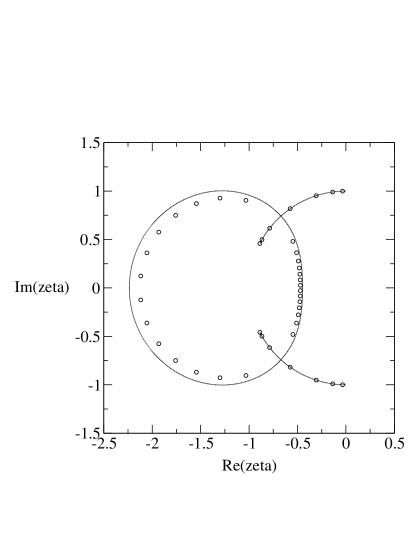
FIG. 2.: Singular locus ${\cal B}$ in the $\zeta$ plane for the free energy of the $q=5/4$ Potts model on the $L_{x}\to\infty$ limit of the $L_{y}=1$ strip with DBC1 boundary conditions. For comparison, zeros of $Z$ for $L_{x}=21$ are shown.

For an interval $q\geq q_{ac}$, there are two O phases, namely the regions surrounded by the oval curve and separated by the arc of the $|\zeta|=1$ circle that passes through $\zeta=-1$. The rest of the $\zeta$ plane is occupied by the complex-temperature extension of the paramagnetic (PM) phase. This type of situation is illustrated in Fig. 3 for $q=(5/4)^{2}$ and Fig. 4 for $q=1.7$.

‘

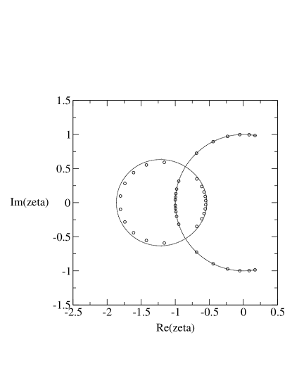
FIG. 3.: Same as Fig. 2 for $q=(5/4)^{2}=1.5625$.

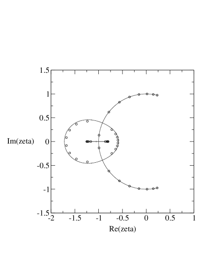
FIG. 4.: Same as Fig. 2 for $q=1.7$.

As $q$ increases further, the two O phases that were contiguous now contract and pull away from each other. This is illustrated in Fig. 5 for $q=1.85$. Eventually, these two O phases pull completely away so that they are no longer contiguous; they are then centered around the endpoints of the line segment. An example is shown in Fig. 6 for $q=1.9$. Here the crossing of the right-hand O phase, i.e. the crossing nearest to the origin, occurs at $\zeta_{t}$ and its inverse is the leftmost crossing of the other O phase.

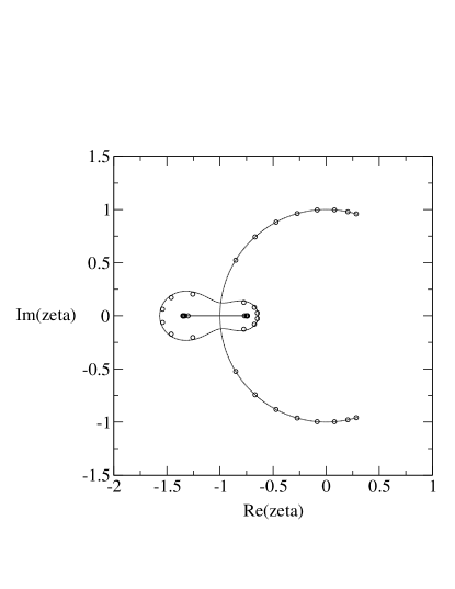
FIG. 5.: Same as Fig. 2 for $q=1.85$.

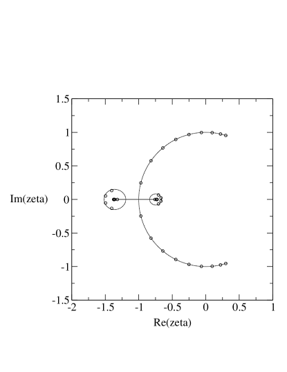
FIG. 6.: Same as Fig. 2 for $q=1.9$.

As $q$ increases to $q=2$, the two O phases contract to points and disappear. One can see this analytically since at $q=2$ the crossing $\zeta_{t}=-1/\sqrt{2}$ coincides with the line segment endpoint $\zeta_{se}=-1/\sqrt{2}$ and similarly for their inverses. In the interval $2<q<9/4=2.25$ the points $\zeta_{t}$ and $\zeta_{t}^{-1}$ are located in the interior of the line segment and do not play a special role. As $q$ increases above $q=9/4$, there ceases to be any real-$q$ solution of the condition $T_{S1}=0$. The locus ${\cal B}$ and complex-temperature phase diagram are shown for $q=3$ in Fig. 7. A topological feature of ${\cal B}$ for this region of $q$, namely the presence of a complex-temperature endpoint of a line segment on the left, is reminiscent of the suggestive possibility of prongs (or perhaps cusps) on ${\cal B}$ for the square-lattice Potts model inferred from the combination of calculations of Fisher zeros and the correlation of the positions of these zeros with locations of complex-temperature singularities that were reliably determined from analyses of low-temperature series expansions in [43] (see also [47, 48]). The angle $\theta_{ae}$ of the upper arc endpoint decreases as $q$ increases, i.e., this endpoint moves toward the point $\zeta=1$ on the real axis. In Table I we list some explicit values of this angle $\theta_{ae}$ as a function of $q$ for (the $L_{x}\to\infty$ limit of) this strip.

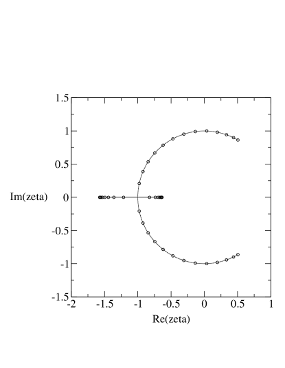
FIG. 7.: Same as Fig. 2 for $q=3$.

TABLE I.: Values of arc endpoint angles $\theta_{ae}$ for various infinite-length finite-width square lattice strips with duality-preserving boundary conditions. The $\theta_{ae}$ values are the same for DBC1 and DBC2.

$L_{y}$	$q=1$	$q=2$	$q=3$	$q=4$	$q=10$
1	$120^{\circ}$	$69.3^{\circ}$	$58.1^{\circ}$	$52.0^{\circ}$	$37.8^{\circ}$
2	$88.8^{\circ}$	$47.7^{\circ}$	$38.8^{\circ}$	$34.1^{\circ}$	$23.7^{\circ}$

As $q$ gets large, the right-hand arc endpoints move down toward the point $\zeta=1$ and the circular arc finally pinches this point in the limit as $q\to\infty$. We calculate the following expansions for the position of the upper arc endpoint for large $q$:

$$\zeta_{ae}=1+iq^{-1/4}-\frac{1}{2}q^{-1/2}+\frac{3}{2^{3}}iq^{-3/4}-\frac{1}{2}q^{-1}-\frac{41}{2^{7}}iq^{-5/4}+\frac{123}{2^{10}}iq^{-7/4}-\frac{1}{2^{3}}q^{-2}+O(q^{-9/4})$$ (41)

(the lower one being the complex conjugate) and, for the right and left endpoints of the line segment. On the left, as $q$ gets large the line segment contracts toward $\zeta=-1$ and finally degenerates to a point at $q=\infty$. We calculate the following expansion for the positions of the endpoints of this line segment for large $q$:

$$\zeta_{se},\zeta_{se}^{-1}=-1\pm q^{-1/4}-\frac{1}{2}q^{-1/2}\mp\frac{3}{2^{3}}q^{-3/4}+\frac{1}{2}q^{-1}\mp\frac{41}{2^{7}}q^{-5/4}$$ (42)

(43)

$$\mp\frac{123}{2^{10}}q^{-7/4}+\frac{1}{2^{3}}q^{-2}+O(q^{-9/4})\ .$$ (44)

Thus, in the limit as $q\to\infty$, ${\cal B}$ becomes the unit circle $|\zeta|=1$.

Going the other way, let us start at $q=\infty$, where ${\cal B}$ is the circle $|\zeta|=1$. As $q$ decreases from infinity, two changes occur immediately in ${\cal B}$: (i) the circle breaks open on the right side, forming two arcs with endpoints at the angles given in (37) that recede away from the real axis, and (ii) a real line segment sprouts out from the point $\zeta=-1$. Feature (i) reflects the quasi-one-dimensional nature of the $L_{x}\to\infty$ limit of this family of strip graphs, since for finite $q$, the free energy of the Potts ferromagnet is analytic for all finite temperatures. This feature does not hold in the thermodynamic limit on the square lattice. As was discussed in [33, 34] for the Ising model and in [43] for the general Potts model, the region around $a=1$, i.e., $v=0$, which is the paramagnetic phase, is not analytically connected to the broken-symmetry, ferromagnetic phase; hence the part of the phase boundary ${\cal B}$ that separates the complex-temperature extensions of the PM phase and FM phases from each other must remain intact as $q$ decreases from infinity. However, the deviation on the left serves as a prototype of the sort of deviations that are suggested by finite-lattice calculations of Fisher zeros for sections of the square lattice [29, 39, 43, 60] and gives some insight, as an exactly calculable example, of how these deviations arise. As $q$ decreases to sufficiently small values, the line segment changes to a region around $\zeta=-1$. As we shall show below, the nature of the deviation on the left can be more complicated for wider strips. Thus, from the point of view of increasing $q$, ${\cal B}$ only becomes the unit circle $|\zeta|=1$ in the limit $q\to\infty$.

We next point out an another important feature of these results. For the $q=3$ case, ${\cal B}$ crosses the real axis at $\zeta=-1/\sqrt{3}$, its inverse $-\sqrt{3}$, and at $\zeta=-1$. Transforming back to the $v$ plane, these points correspond to $v=-1$, $v=-3$, and $v=-\sqrt{3}$, respectively. The crossing at $v=-1$, i.e., $a=0$, connotes a zero-temperature critical point of the $q=3$ Potts antiferromagnet on this infinite-length $L_{y}=1$ strip [87, 88]. This is very interesting, since this model also has a zero-temperature critical point on the (infinite) square lattice. Thus, an infinite-length strip with width $L_{y}=1$ already exhibits a feature of the Potts antiferromagnet on the full square lattice. As will be seen below, this is also true of the other widths $L_{y}=2,3$ for which we have obtained exact solutions for the Potts model free energy. The crossing at $v=-3$, i.e., $a=-2$, is a complex-temperature singular point that is the dual image of $a=0$ and, by duality, the singularity in the free energy is the same as at the physical zero-temperature critical point, in accordance with the general discussion in [45] relating physical and complex-temperature singularities by duality. It is instructive to view the locus ${\cal B}$ in the complex $\zeta$ or $v$ plane for fixed $q$ as a slice of the singular subset in the full ${\mathbb{C}}^{2}$ space defined by the pair of variables or $(q,v)$. Thus, the crossing of ${\cal B}$ at $v=-1$ for $q=3$ is the point $(q,v)=(3,-1)$ and corresponds to the crossing of the slice of ${\cal B}$ at $q=3$ in the $q$ plane at fixed $v=-1$. This is precisely the $q_{c}$ that we found previously in our study of chromatic polynomials and their asymptotic limits and loci ${\cal B}$ for this family of graphs in [77]. It will be recalled that we found that this $q_{c}=3$ value was universal for all of the widths $1\leq L_{y}\leq 4$ for which we calculated exact solutions for the chromatic polynomial and resultant ${\cal B}$. As we shall show below, this corresponds to the feature that for each of the widths of strips that we study here, ${\cal B}$ passes through $v=-1$, i.e., $\zeta=-1/\sqrt{3}$ (and, by duality, its inverse, $\zeta=-\sqrt{3}$) for $q=3$.

For the Ising case $q=2$, ${\cal B}$ crosses the $v$ axis at $v=-1$ and the dual image $v=-2$. The crossing at $v=-1$ connotes a zero-temperature critical point for the Ising antiferromagnet on the $L_{x}\to\infty$ limit of this graph.

We have also calculated Fisher zeros for the strips with DBC1 and $L_{y}=2,3$. A typical example is $L_{y}=3$, $q=4$, shown in Fig. 8. For lack of space we do not show the others here, but they are available upon request.

FIG. 8.: Complex-temperature Fisher zeros in the $\zeta$ plane for the $q=4$ Potts model on the $L_{y}=3$ strip with DBC1 boundary conditions with $L_{x}=21$ ($n=64$).

IV $L_{y}=1$, DBC2

To elucidate the dependence of ${\cal B}$ on the self-dual boundary conditions, we consider the $L_{y}=1$ strips with DBC2. We shall denote this family generically as $L$, and $L,1$ or $L1$ to specify the width. The number of $\lambda$’s in the form (15), is, from [77],

$$N_{Z,L,L_{y},\lambda}={2L_{y}+1\choose L_{y}+1}\ .$$ (45)

In particular, for $L_{y}=1$, this gives $N_{Z,L,1,\lambda}=3$. We find

$$\lambda_{L,1,1}=v\ ,\quad\lambda_{L,1,2}=\lambda_{S,1,1}\ ,\quad\lambda_{L,1,3}=\lambda_{S,1,2}\ .$$ (46)

The corresponding coefficients in (15) are

$$c_{L1,1}=\kappa^{(2)}=q(q-2)$$ (47)

$$c_{L1,j}=\kappa^{(1)}=q\quad{\rm for}\quad j=2,3$$ (48)

where [77]

$$\kappa^{(d)} = 2\Bigg{[}U_{2d}\Big{(}\frac{\sqrt{q}}{2}\Big{)}-T_{2d}\Big{(}\frac{\sqrt{q}}{2}\Big{)}\Bigg{]}$$ (49)

$$= \sqrt{q}\ U_{2d-1}\Big{(}\frac{\sqrt{q}}{2}\Big{)}$$ (51)

$$= \sum_{j=0}^{d-1}(-1)^{j}{2d-1-j\choose j}q^{d-j}$$ (53)

where $T_{n}(x)$ and $U_{n}(x)$ are the Chebyshev polynomials of the first and second kinds. Structural properties of $Z(G,q,v)$ for these strips have interesting connections with Temperley-Lieb algebras and Bratteli diagrams, which were pointed out in [77].

In Figs. 9-13 we show the locus ${\cal B}$ and associated complex-temperature phase diagram in the $\zeta$ plane for the values $q=2$, 3, 4, 5, and 100. (Note that the locus ${\cal B}$ shown in Fig. 9 is ${\cal B}_{nq}$.) The arc endpoints of the portion of ${\cal B}$ lying on the circle $|\zeta|=1$ are the same as for the ($L_{x}\to\infty$ limit of the) $L_{y}=1$ strip with DBC1, i.e., $\zeta_{ae},\zeta_{ae}^{*}$ given in eq. (36). The reason for this property is that in this area of the $\zeta$ plane the locus ${\cal B}$ is determined by the equality in magnitude of two terms, $\lambda_{L,1,2}$ and $\lambda_{L,1,3}$, which are common to the partition functions for DBC1 and DBC2. In our calculations for $L_{y}=2,3$ we have found the same property to hold, so that for a given width $L_{y}$ and value of $q$, for the strips considered here, the locations of the right-hand arc endpoints are independent of whether one uses DBC1 or DBC2 boundary conditions. However, there is an interval in $q$ for which $\lambda_{L,1,1}$ is dominant in the vicinity of $\zeta=-1$, and this leads to at least one complex-temperature O phase (in the nomenclature of [33]). Figs. 10 and 11 illustrate this for the cases $q=3$ and $q=4$. One observes complex-conjugate triple points on ${\cal B}$ for $q=3$. An exactly solved case of a complex-temperature phase boundary exhibiting such a triple point was given in [42], where it was shown how this triple point results from three curves on ${\cal B}$ coming together such that as one travels along a given curve, beyond the intersection point the $\lambda$’s that were leading and degenerate in magnitude on this curve are no longer leading, so that their degeneracy is not relevant to ${\cal B}$. In our exact calculations of ${\cal B}$ in the $q$ plane for $n\to\infty$ limits of chromatic polynomials we have found a number of such triple points (e.g., [79]-[84],[78]). Considering ${\cal B}$ as the union of the various curves and line segments that comprise it, this is a multiple point (intersection point) on ${\cal B}$ since it lies on multiple branches of ${\cal B}$. In a different nomenclature in which one considers each of the algebraic curves individually, including the portions where the pairs of degenerate-magnitude $\lambda$’s are not dominant so that these portions are not on ${\cal B}$, then such triple points are not multiple points on each individual algebraic curve, since these individual curves pass through the triple point as shown in Fig. 2 in [42] (see also [85, 86]).

In general, as we did for the DBC1 strips, we find that for any finite $q$ no matter how large, ${\cal B}$ deviates from the circle $|\zeta|=1$. As discussed above, the gap that opens in the circle in the vicinity of $\zeta=1$ is a property that is special to the quasi-one-dimensional nature of these infinite-length, finite width strips. However, just as our previous exact results showed that certain complex-temperature properties of quasi-one-dimensional spin models were similar to those of the same models in 2D [41, 53, 54, 56, 57, 58], so also the deviations in the region around $\zeta=-1$ are indicative of what can happen in 2D in this case. Note that for $q>1$, the point $\zeta=-1$, i.e., $v=-\sqrt{q}$, is a complex-temperature, rather than physical, point. We can now use our results to address the issue of the radius of convergence of the $1/q$ expansion as regards the form of ${\cal B}$. In general, if an expansion of some quantity in a variable $\epsilon$ has a finite radius of convergence $\epsilon_{c}$, then, roughly speaking, the behavior for $|\epsilon|<\epsilon_{c}$ should be qualitatively the same as for $\epsilon=0$. Our results suggest that, at least for the infinite-length finite-width strips, the $1/q$ expansion has zero radius of convergence insofar as properties of the locus ${\cal B}$ are concerned. This follows since ${\cal B}$ in the $\zeta$ plane differs qualitatively for any nonzero value of $1/q$ from its form at $1/q=0$. We know that the deviation near $\zeta=1$, i.e. the physical PM-FM transition temperature given by $v_{c}=\sqrt{q}$, that occurs for these quasi-one-dimensional strips will be absent in 2D. However, the deviation in the vicinity of the complex-temperature point $\zeta=-1$ should be a more general feature, not limited to the quasi-one-dimensional nature of the strips considered here. This inference follows from (i) our previous experience comparing exactly determined complex-temperature features of Ising model phase diagrams for infinite-length strips and in 2D, (ii) the observed scatter of Fisher zeros in 2D [29, 38, 43] in this complex-temperature region, and (iii) reliable determinations of locations of complex-temperature singularities via analyses of low-temperature series [43, 45, 47, 48] and the correlation of these with points on ${\cal B}$ [33, 37, 43, 47, 48]. Hence for the locus ${\cal B}$, our present exact results suggest that the $1/q$ expansion has zero radius of convergence. We emphasize that this does not reduce the value of these large-$q$ expansions, since the point where the deviation occurs is generically a complex-temperature point, and this type of deviation does not occur near the physical PM-FM phase transition point. Indeed, large-$q$ expansions yield excellent agreement with Monte Carlo measurements of thermodynamic quantities in the Potts model [62, 64] and also for the ground state degeneracy $W(q)$ in the $T=0$ Potts antiferromagnet [73],[66]-[72]. Furthermore, it is easily checked that the dominant term $\lambda$ that determines the free energy on the strips that we consider does have a well-defined large-$q$ expansion (in the variable $1/\sqrt{q}$). For example, for $L_{y}=1$ with DBC1 or DBC2, removing the leading factor of $q$, we have the expansion for $q^{-1}\lambda_{S,1,1}$ for large $q$:

$$q^{-1}\lambda_{S,1,1} = 1+2vq^{-1}+v^{2}(v+1)q^{-2}+v^{3}(v^{2}-1)q^{-3}+O(q^{-4})$$ (54)

$$= 1+\frac{\zeta(\zeta^{2}-2)}{\zeta^{2}-1}q^{-1/2}-\frac{\zeta^{2}(\zeta^{2}+\zeta-1)(\zeta^{2}-\zeta-1)}{(\zeta^{2}-1)^{3}}q^{-1}$$ (58)

$$+\frac{\zeta^{3}(\zeta^{2}+1)(\zeta^{2}+\zeta-1)(\zeta^{2}-\zeta-1)}{(\zeta^{2}-1)^{5}}q^{-3/2}+O(q^{-2})\ .$$

Note the poles at $\zeta=\pm 1$ in this expansion. Parenthetically, we note that our findings here concerning the large-$q$ expansion are not related to our earlier studies of families of graphs for which $W(q)$ has no large-$q$ expansion [73, 89, 90, 81, 52] (see also [91]) since in those cases, the breakdown of the $1/q$ expansion is equivalent to the property that the singular locus ${\cal B}$ is noncompact in the $q$ plane, passing through the origin of the $1/q$ plane. This sort of breakdown does not occur for the present families of graphs, as is clear from the fact that ${\cal B}$ is compact in the $q$ plane, shown in [77] and above.

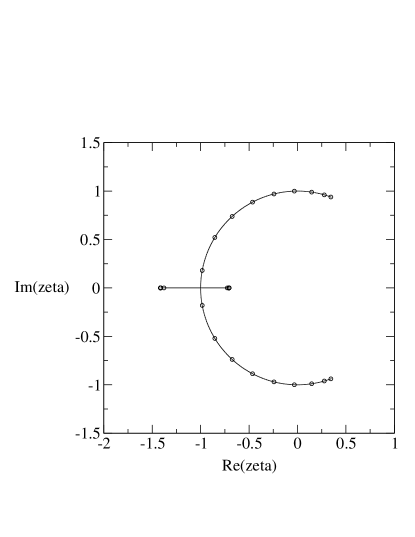
FIG. 9.: Singular locus ${\cal B}$ in the $\zeta$ plane for the free energy of the $q=2$ Potts model on the $L_{x}\to\infty$ limit of the $L_{y}=1$ strip DBC2 boundary conditions. For comparison, zeros of $Z$ for $L_{x}=20$ are shown.

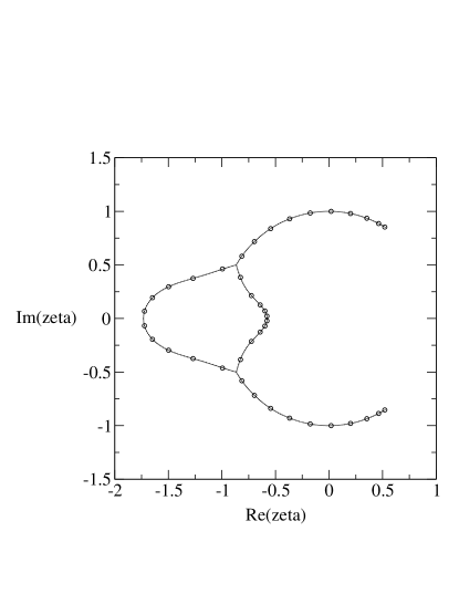
FIG. 10.: Same as Fig. 9 for $q=3$.

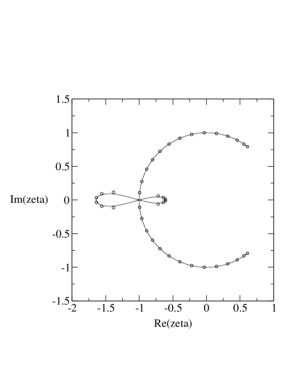
FIG. 11.: Same as Fig. 9 for $q=4$.

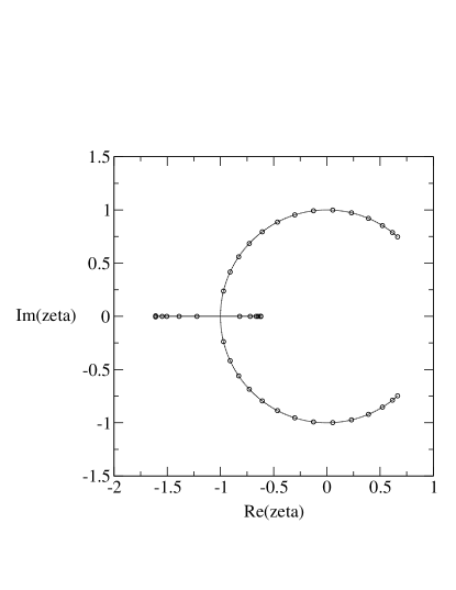
FIG. 12.: Same as Fig. 9 for $q=5$.

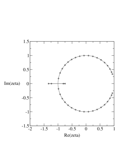
FIG. 13.: Same as Fig. 9 for $q=100$.

V Wider Strips

We have also calculated $Z(G,q,v)$ for arbitrary $q$ and $v$ for wider strips with $L_{y}=2$ and $L_{y}=3$, for which our general formulas (18) and (45) from [77] yield for the number of $\lambda$’s the results $N_{Z,DBC1,2,\lambda}=5$, $N_{Z,DBC2,2,\lambda}=10$, $N_{Z,DBC1,3,\lambda}=14$, and $N_{Z,DBC2,3,\lambda}=35$. The analytic expressions for the $\lambda$’s are too lengthy to list here. In several figures below we show plots of Fisher zeros in the $\zeta$ plane for various values of $q$.

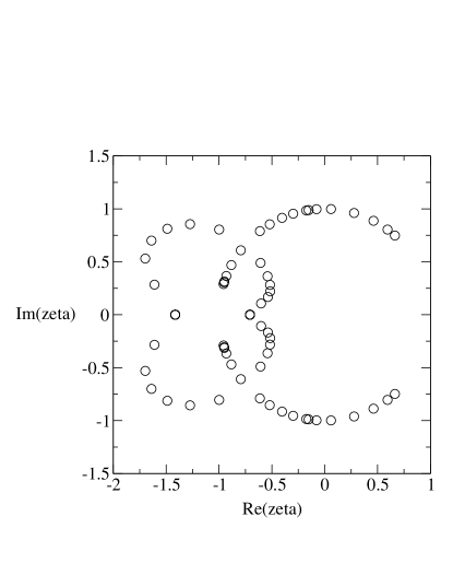
FIG. 14.: Complex-temperature Fisher zeros in the $\zeta$ plane for the $q=2$ Potts model on the $L_{y}=2$ strip with DBC2 boundary conditions with $L_{x}=20$ ($n=40$).

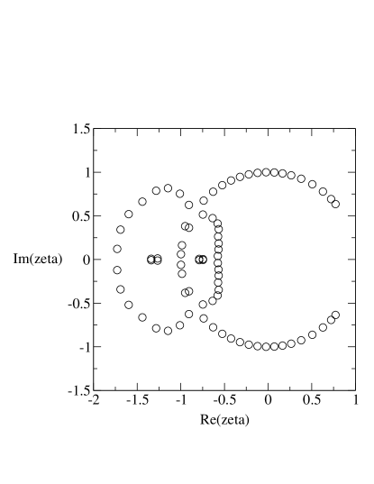
FIG. 15.: Same as Fig. 14 for $q=3$.

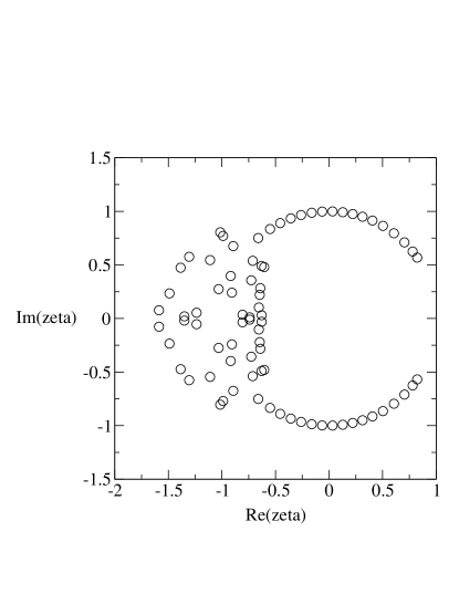
FIG. 16.: Same as Fig. 14 for $q=4$.

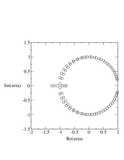
FIG. 17.: Same as Fig. 14 for $q=100$.

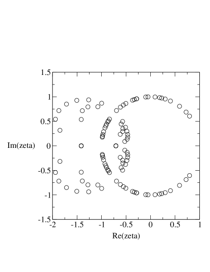
FIG. 18.: Complex-temperature Fisher zeros in the $\zeta$ plane for the $q=2$ Potts model on the $L_{y}=3$ strip with DBC2 boundary conditions with $L_{x}=20$ ($n=60$).

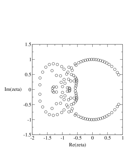
FIG. 19.: Same as Fig. 19 for $q=3$.

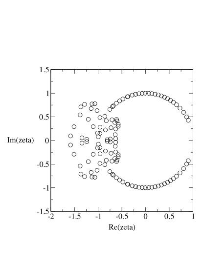
FIG. 20.: Same as Fig. 20 for $q=4$.

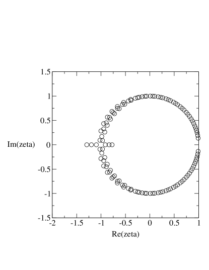
FIG. 21.: Same as Fig. 18 for $q=100$.

It is interesting to note that the simplification of the complex-temperature phase diagram for the Potts model to the circle $|\zeta|=1$ for $q\to\infty$ proved in [39] and studied further here with exact results is somewhat similar to the simplification of the complex-temperature phase diagram for the 2D spin-$s$ Ising model in the limit $s\to\infty$ to the circle $|u_{s}|=1$ in the plane of the Boltzmann variable $u_{s}=e^{-K/s^{2}}$ [92, 93, 41]. In both cases, the approach to the limit is singular in the sense that there are deviations from the asymptotic locus.

VI Conclusions

In summary, we have presented exact calculations of the Potts model partition function $Z(G,q,v)$ on self-dual strip graphs $G$ of the square lattice with fixed width $L_{y}$ and arbitrarily great length $L_{x}$ with two types of boundary conditions. In the infinite-length limit we have studied the resultant complex-temperature phase diagram. In particular, we have considered the widths $L_{y}=1,2,3$. We have used these results to study the approach to the large-$q$ limit of ${\cal B}$, where this locus is the unit circle $|\zeta|=1$. We find that, for a given $L_{y}$ and set of self-dual boundary conditions, a portion of ${\cal B}$ lies on this unit circle, while for any finite $q$, a portion deviates from this circle. For the strips considered here we find that the right-hand arc endpoints on the circle are independent of whether the longitudinal boundary conditions are periodic or free and to curve around and pinch the real axis at $\zeta=1$ as $q\to\infty$. For a fixed value of $q$, as $L_{y}$ increases, the right-hand arc endpoints move closer to $\zeta=1$. On the left, the nature of the complex-temperature phase diagram was found to depend in detail on both the type of boundary conditions and the width of the strip. As $q\to\infty$, the deviations typically include real line segments as well as possible O phases. One feature was found for each width considered, namely that for the DBC2 strips, for $q=3$, ${\cal B}$ crosses the $\zeta$ at $\zeta=-1/\sqrt{3}$ and at $-\sqrt{3}$. We showed that this is equivalent to the fact that for $v=-1$, each of the infinite-length strips that we studied in [77] with $1\leq L_{y}\leq 4$ and DBC2 had $q_{c}=3$ as for the infinite square lattice. As discussed, the gap in the locus ${\cal B}$ that opens around $\zeta=1$ as $1/q$ increases above zero is a consequence of the quasi-one-dimensional nature of the strips. However, the behavior in the $Re(\zeta)<0$ region near $\zeta=-1$ can give some insight as to how ${\cal B}$ could behave for large $q$ on the infinite square lattice.

Acknowledgment: This research was partially supported by the NSF grant PHY-97-22101.

VII Appendix

A General

The most compact way to express a Potts model partition function $Z(G,q,v)$ is often in terms of the corresponding Tutte polynomial $T(G,x,y)$. For the reader’s convenience, we recall the definition of the Tutte polynomial and some basic formulas relating these functions here (e.g., [53]). For an arbitrary graph $G$ the Tutte polynomial of $G$, $T(G,x,y)$, is given by [5]-[7]

$$T(G,x,y)=\sum_{G^{\prime}\subseteq G}(x-1)^{k(G^{\prime})-k(G)}(y-1)^{c(G^{\prime})}$$ (59)

where the spanning subgraph $G^{\prime}$ was defined in the introduction, and we recall that $k(G^{\prime})$, $e(G^{\prime})$, and $n(G^{\prime})=n(G)$ denote the number of components, edges, and vertices of $G^{\prime}$, where

$$c(G^{\prime})=e(G^{\prime})+k(G^{\prime})-n(G^{\prime})$$ (60)

is the number of independent circuits in $G^{\prime}$. As stated in the text, $k(G)=1$ for the graphs of interest here. Now let

$$x=1+\frac{q}{v}\ ,\quad y=a=v+1$$ (61)

so that

$$q=(x-1)(y-1)\ .$$ (62)

Then

$$Z(G,q,v)=(x-1)^{k(G)}(y-1)^{n(G)}T(G,x,y)\ .$$ (63)

For a planar graph $G$ the Tutte polynomial satisfies the duality relation

$$T(G,x,y)=T(G^{*},y,x)$$ (64)

where $G^{*}$ is the (planar) dual to $G$. As discussed in [53], the Tutte polynomial for recursively defined graphs comprised of $m$ repetitions of some subgraph has the form

$$T(G_{m},x,y)=\sum_{j=1}^{N_{\lambda}}c_{T,G,j}(\lambda_{T,G,j})^{m}\ .$$ (65)

One special case of the Tutte polynomial of particular interest is the chromatic polynomial $P(G,q)$. This is obtained by setting $y=0$, i.e., $v=-1$, so that $x=1-q$; the correspondence is $P(G,q)=(-q)^{k(G)}(-1)^{n}T(G,1-q,0)$.

B Strips with DBC1

The generating function representation for the Tutte polynomial for the strip $S_{m}$ of the square lattice with length $L_{x}=m+1$ vertices, i.e., $m$ edges in each horizontal row, and of width $L_{y}$, with duality preserving boundary conditions of type 1, is

$$\Gamma_{T}(S_{m},L_{y},x,y,z)=\sum_{m=0}^{\infty}T(S_{m},L_{y},x,y)z^{m}\ .$$ (66)

We have

$$\Gamma_{T}(S,L_{y},x,y;z)=\frac{{\cal N}_{T}(S,L_{y},x,y,z)}{{\cal D}_{T}(S,L_{y},x,y,z)}\ .$$ (67)

For $L_{y}=1$ we find

$${\cal N}_{T}(S,1,x,y,z)=(x+y)-xyz$$ (68)

$${\cal D}_{T}(S,1,x,y,z) = 1-(1+x+y)z+xyz^{2}$$ (69)

$$= \prod_{j=1}^{2}(1-\lambda_{T,S,1,j}z)$$ (71)

with

$$\lambda_{T,S,1,(1,2)}=\frac{1}{2}\biggl{[}1+x+y\pm\Bigl{(}1+2(x+y)+(x-y)^{2}\Bigr{)}^{1/2}\biggr{]}\ .$$ (72)

$$T(S_{m},x,y)=\biggl{[}\frac{A_{T,S,0}\lambda_{T,S,1}+A_{T,S,1}}{\lambda_{T,S,1}-\lambda_{T,S,2}}\biggr{]}(\lambda_{T,S,1})^{m}+\biggl{[}\frac{A_{T,S,0}\lambda_{T,S,2}+A_{T,S,1}}{\lambda_{T,S,2}-\lambda_{T,S,1}}\biggr{]}(\lambda_{T,S,2})^{m}\ .$$ (73)

For $L_{y}=2$ we find

$${\cal N}_{T}(S,2,x,y,z)=A_{S2,0}+A_{S2,1}z+A_{S2,2}z^{2}+A_{S2,3}z^{3}+A_{S2,4}z^{4}$$ (74)

where

$$A_{S2,0}=x+y+xy+x^{2}+y^{2}$$ (75)

$$A_{S2,1}=-\bigg{[}x+y+2(x^{2}+y^{2})+3xy+5xy(x+y)+xy(x^{2}+y^{2})+x^{3}+y^{3}+(xy)^{2}\bigg{]}$$ (76)

$$A_{S2,2}=xy\bigg{[}3(x+y)+4(x^{2}+y^{2})+6xy+3xy(x+y)+x^{3}+y^{3}+(xy)^{2}\bigg{]}$$ (77)

$$A_{S2,3}=-(xy)^{2}\bigg{[}2(x+y)+x^{2}+y^{2}+3xy+xy(x+y)\bigg{]}$$ (78)

$$A_{S2,4}=(xy)^{4}$$ (79)

$${\cal D}_{T}(S,2,x,y,z)=1+b_{S2,1}z+b_{S2,2}z^{2}+b_{S2,3}z^{3}+b_{S2,4}z^{4}+b_{S2,5}z^{5}$$ (80)

where

$$b_{S2,1}=-\bigg{[}3(1+x+y)+xy+x^{2}+y^{2}\bigg{]}$$ (81)

$$b_{S2,2}=1+3(x+y)+3(x^{2}+y^{2})+8xy+(x^{3}+y^{3})+5xy(x+y)+xy(x^{2}+y^{2})+(xy)^{2}$$ (82)

$$b_{S2,3}=-xy\bigg{[}3+5(x+y)+4(x^{2}+y^{2})+6xy+(x^{3}+y^{3})+3xy(x+y)+(xy)^{2}\bigg{]}$$ (83)

$$b_{S2,4}=(xy)^{2}(1+x)(1+y)(1+x+y)$$ (84)

$$b_{S2,5}=-(xy)^{4}\ .$$ (85)

For $L_{y}=3$ our general results in [77] yield the result that there are 14 terms, and we find that the $\lambda_{T,S,3,j}$’s are roots of an algebraic equation of degree 14. This is too lengthy to record here, but is available upon request.

C Strips with DBC2

We have

$$T(L_{m},L_{y},x,y)=\sum_{j=1}^{N_{T,L,L_{y},\lambda}}c_{T,L,L_{y},j}(\lambda_{T,L,L_{y},j})^{m}$$ (86)

where $N_{T,L,L_{y},\lambda}=N_{Z,L,L_{y},\lambda}$, and our general formula for this number, from [77] was given in (45).

1 $L_{y}=1$

We have $N_{T,L,1,\lambda}=3$ and

$$\lambda_{T,L,1,1}=1$$ (87)

$$\lambda_{T,L,1,j}=\lambda_{T,S,1,j-1}\quad{\rm for}\ j=2,3$$ (88)

where $\lambda_{T,S,1,1}$ and $\lambda_{T,S,1,2}$ were given in eq. (72). The corresponding coefficients are

$$c_{T,L,1,1}=q^{-1}\kappa^{(2)}=q-2=xy-x-y-1$$ (89)

$$c_{T,L,j}=q^{-1}\kappa^{(1)}=1\quad{\rm for}\quad j=2,3$$ (90)

where $\kappa^{(d)}$ was defined in eq. (53) in the text.

2 $L_{y}=2$

We have $N_{T,L,2,\lambda}=10$. The term $\lambda_{T,L,2,1}$ is

$$\lambda_{T,L,2,1}=1\ .$$ (91)

The $\lambda_{T,L,2,j}$ for $2\leq j\leq 5$ are solutions to the equation

$$\xi^{4}-\Big{[}2(x+y)+3\Big{]}\xi^{3}+\Big{[}x^{2}+y^{2}+3(x+y)+4xy+1\Big{]}\xi^{2}$$ (92)

(93)

$$-xy\Big{[}2(x+y)+3\Big{]}\xi+(xy)^{2}=0\ .$$ (94)

The $\lambda_{T,L,2,j}$ for $6\leq j\leq 10$ are solutions to the equation

$$\xi^{5}+b_{S2,1}\xi^{4}+b_{S2,2}\xi^{3}+b_{S2,3}\xi^{2}+b_{S2,4}\xi+b_{S2,5}=0\ .$$ (95)

The corresponding coefficients are

$$c_{T,L,2,1}=q^{-1}\kappa^{(3)}=(q-1)(q-3)=(xy-x-y)(xy-x-y-2)$$ (96)

$$c_{T,L,2,j}=q^{-1}\kappa^{(2)}=q-2=xy-x-y-1\quad{\rm for}\quad 2\leq j\leq 5$$ (97)

$$c_{T,L,2,j}=q^{-1}\kappa^{(1)}=1\quad{\rm for}\quad 6\leq j\leq 10\ .$$ (98)

3 $L_{y}=3$

Here our general formulas in [77] yield the results that there are 35 terms in all, comprised of (i) one term with coefficient $q^{-1}\kappa^{(4)}$, namely, $\lambda_{T,L,3,1}=1$, (ii) six terms $\lambda_{T,L,3,j}$, $2\leq j\leq 7$, with coefficient $q^{-1}\kappa^{(3)}$, (iii) 14 terms $\lambda_{T,L,3,j}$ for $8\leq j\leq 21$ with coefficient $q^{-1}\kappa^{(2)}$, and (iv) 14 terms $\lambda_{T,L,3,j}$ with $22\leq j\leq 35$ with coefficient $q^{-1}\kappa^{(1)}$. The terms in (ii) are roots of the sixth-degree equation

$$\xi^{6}-(3x+3y+5)\xi^{5}+(3x^{2}+9yx+10x+3y^{2}+10y+6)\xi^{4}$$ (99)

(100)

$$-(x^{3}+9yx^{2}+5x^{2}+9y^{2}x+20yx+6x+y^{3}+5y^{2}+6y+1)\xi^{3}$$ (101)

(102)

$$+xy(3x^{2}+9yx+10x+3y^{2}+10y+6)\xi^{2}-x^{2}y^{2}(3x+3y+5)\xi+x^{3}y^{3}=0\ .$$ (103)

The equation of degree 14 for the $\lambda_{T,L,3,j}$ with coefficient $q^{-1}\kappa^{(1)}$ is the same as the single degree-14 equation for the terms in the $L_{y}=3$ strip with DBC1. Both this and the other degree-14 equation are too lengthy to list here, but can be provided at request.

D Special Values of Tutte Polynomials

For a given graph $G=(V,E)$, at certain special values of the arguments $x$ and $y$, the Tutte polynomial $T(G,x,y)$ yields quantities of basic graph-theoretic interest [7]-[10]. We recall some definitions: a spanning subgraph was defined at the beginning of the paper; a tree is a connected graph with no cycles; a forest is a graph containing one or more trees; and a spanning tree is a spanning subgraph that is a tree. We recall that the graphs $G$ that we consider are connected. Then the number of spanning trees of $G$, $N_{ST}(G)$, is

$$N_{ST}(G)=T(G,1,1)\ ,$$ (104)

the number of spanning forests of $G$, $N_{SF}(G)$, is

$$N_{SF}(G)=T(G,2,1)\ ,$$ (105)

the number of connected spanning subgraphs of $G$, $N_{CSSG}(G)$, is

$$N_{CSSG}(G)=T(G,1,2)\ ,$$ (106)

and the number of spanning subgraphs of $G$, $N_{SSG}(G)$, is

$$N_{SSG}(G)=T(G,2,2)\ .$$ (107)

Since the graphs that we consider are self-dual, and using the symmetry relation (64), we have

$$N_{SF}(G)=N_{CSSG}(G^{*})=N_{CSSG}(G)\ .$$ (108)

From our calculations of Tutte polynomials, we find the following results.

E $L_{y}=1$, DBC1

$$N_{ST}(S1_{m})=\Bigg{(}1+\frac{2\sqrt{5}}{5}\ \Bigg{)}\Bigg{(}\frac{3+\sqrt{5}}{2}\ \Bigg{)}^{m}+\Bigg{(}1-\frac{2\sqrt{5}}{5}\ \Bigg{)}\Bigg{(}\frac{3-\sqrt{5}}{2}\ \Bigg{)}^{m}$$ (109)

$$N_{SF}(S1_{m})=N_{CSSG}(S1_{m})=\Bigg{(}\frac{3}{2}+\sqrt{2}\Bigg{)}(2+\sqrt{2}\ )^{m}+\Bigg{(}\frac{3}{2}-\sqrt{2}\Bigg{)}(2-\sqrt{2}\ )^{m}$$ (110)

$$N_{SSG}(S1_{m})=2^{e(S1_{m})}=2^{2(m+1)}\ .$$ (111)

Since these quantities grow exponentially, it is natural to define an associated quantity that measures this growth [94, 95, 96]. In particular, for the number of spanning trees, we define

$$z_{\{G\}}=\lim_{n\to\infty}n^{-1}\ln N_{ST(\{G\})}\ .$$ (112)

For the present $L_{y}=1$, DBC1 strips, we thus have $z=\ln[(3+\sqrt{5}\ )/2]\simeq 0.9624$. A general upper bound on the number of spanning trees of a graph $G$ is [97]

$$N_{ST}(G)\leq\frac{1}{n}\biggl{(}\frac{2|E|}{n-1}\biggr{)}^{n-1},$$ (113)

For the present $L_{y}=1$, DBC1 strips, this gives the upper bound $z<2\ln 2\simeq 1.386$, which is seen to be satisfied by our result.

F $L_{y}=1$, DBC2

$$N_{ST}(L1_{m})=-2+\Bigg{(}\frac{3+\sqrt{5}}{2}\ \Bigg{)}^{m}+\Bigg{(}\frac{3+\sqrt{5}}{2}\ \Bigg{)}^{m}$$ (114)

$$N_{SF}(L1_{m})=N_{CSSG}(L1_{m})=-2+(2+\sqrt{2}\ )^{m}+(2-\sqrt{2}\ )^{m}$$ (115)

$$N_{SSG}(L1_{m})=2^{e(L1_{m})}=2^{2m}\ .$$ (116)

As discussed before [53, 96], for a given $L_{y}$ and set of transverse boundary conditions, the value of $z$ is the same, independent of whether the longitudinal boundary conditions are free, as in DBC1 or periodic, as for DBC2.

G $L_{y}=2$, DBC2

$$N_{ST}(L2_{m})=3-2\sum_{j=2}^{5}(\lambda_{T,L,2,j}(1,1)\ )^{m}+\sum_{j=6}^{10}(\lambda_{T,L,2,j}(1,1)\ )^{m}$$ (117)

where $\lambda_{T,L,2,j}(1,1)$, $2\leq j\leq 5$ and $6\leq j\leq 10$ are the roots of eq. (94) and eq. (95), respectively, for $x=1,y=1$, viz., $\xi^{4}-7\xi^{3}+13\xi^{2}-7\xi+1=0$, and $(\xi-1)(\xi^{4}-11\xi^{3}+25\xi^{2}-11\xi+1)=0$.

$$N_{SF}(L2_{m})=N_{CSSG}(L2_{m}) = 3-2\Biggl{[}\Bigl{(}\frac{3+\sqrt{5}}{2}\ \Bigr{)}^{m}+\Bigl{(}\frac{3-\sqrt{5}}{2}\ \Bigr{)}^{m}+(3+\sqrt{5}\ )^{m}$$ (118)

$$+ (3-\sqrt{5}\ )^{m}\Biggr{]}+\sum_{j=6}^{10}(\lambda_{T,L,2,j}(2,1)\ )^{m}$$ (120)

where $\lambda_{T,L,2,j}(2,1)$, $6\leq j\leq 10$ are the roots of eq. (95) for $x=2,y=1$, viz., $\xi^{5}-19\xi^{4}+94\xi^{3}-162\xi^{2}+96\xi-16=0$.

$$N_{SSG}(L2_{m})=2^{e(L2_{m})}=2^{4m}\ .$$ (121)

Hence, in particular, for spanning trees, we find $z\simeq 1.044$ for $L_{y}=2$. It is straightforward to use our exact calculations of Tutte polynomials for $L_{y}=3$ with DBC1 and DBC2 boundary conditions to list similar results for spanning trees, etc.

REFERENCES

- [1] R. B. Potts, Proc. Camb. Phil. Soc. 48 106 (1952).
- [2] F. Y. Wu, Rev. Mod. Phys. 54 (1982) 235.
- [3] R. J. Baxter, Exactly Solved Models in Statistical Mechanics (Wiley, New York, 1982).
- [4] P. W. Kasteleyn and C. M. Fortuin, J. Phys. Soc. Jpn. 26 (1969) (Suppl.) 11; C. M. Fortuin and P. W. Kasteleyn, Physica 57 (1972) 536.
- [5] W. T. Tutte, Can. J. Math. 6 (1954) 80.
- [6] W. T. Tutte, J. Combin. Theory 2 (1967) 301.
- [7] W. T. Tutte, “Chromials”, in Lecture Notes in Math. v. 411 (1974) 243; Graph Theory, vol. 21 of Encyclopedia of Mathematics and Applications (Addison-Wesley, Menlo Park, 1984).
- [8] N. L. Biggs, Algebraic Graph Theory (2nd ed., Cambridge Univ. Press, Cambridge, 1993).
- [9] D. J. A. Welsh, Complexity: Knots, Colourings, and Counting, London Math. Soc. Lect. Note Ser. 186 (Cambridge University Press, Cambridge, 1993).
- [10] B. Bollobás, Modern Graph Theory (Springer, New York, 1998).
- [11] C. N. Yang and T. D. Lee, Phys. Rev. 87, 404 (1952); T. D. Lee and C. N. Yang, ibid. 87, 410 (1952).
- [12] M. E. Fisher, Lectures in Theoretical Physics (Univ. of Colorado Press, 1965), vol. 7C, p. 1.
- [13] C. Domb and A. J. Guttmann, J. Phys. C 3, 1652 (1970).
- [14] R. Abe, Prog. Theor. Phys. 38, 322 (1967).
- [15] S. Ono, Y. Karaki, M. Suzuki, and C. Kawabata, J. Phys. Soc. Jpn. 25, 54 (1968).
- [16] H. Brascamp and H. Kunz, J. Math. Phys. 15, 65 (1974).
- [17] R. Pearson, Phys. Rev. B 26, 6285 (1982).
- [18] C. Itzykson, R. Pearson, and J. B. Zuber, Nucl. Phys. B220, 415 (1983).
- [19] J. Stephenson and R. Couzens, Physica 129A, 201 (1984).
- [20] W. van Saarloos and D. Kurtze, J. Phys. A 17, 1301 (1984).
- [21] D. Wood, J. Phys. A: Math. Gen. 18 L481 (1985).
- [22] J. M. Maillard and R. Rammal, J. Phys. A 16, 353 (1983).
- [23] P. Martin and J. M. Maillard, J. Phys. A 19, L547 (1986).
- [24] P. Martin, J. Phys. A 19, 3267 (1986).
- [25] P. Martin, J. Phys. A 20, L601 (1986).
- [26] J. Stephenson, Physica 136A, 147 (1986).
- [27] J. Stephenson, J. Phys. A 20, 4513 (1987).
- [28] G. Marchesini and R. Shrock, Nucl. Phys. B318, 541 (1989).
- [29] P. P. Martin, Potts Models and Related Problems in Statistical Mechanics (World Scientific, Singapore, 1991).
- [30] R. Abe, T. Dotera, and T. Ogawa, Prog. Theor. Phys. 85, 509 (1991).
- [31] P. Damgaard and U. Heller, Nucl. Phys. B 410, 494 (1993).
- [32] I. G. Enting, A. J. Guttmann, and I. Jensen, J. Phys. A 27, 6963 (1994).
- [33] V. Matveev and R. Shrock, J. Phys. A 28, 1557 (1995).
- [34] V. Matveev and R. Shrock, J. Phys. A 28, 5235 (1995).
- [35] V. Matveev and R. Shrock, J. Phys. A 28, 4859 (1995).
- [36] V. Matveev and R. Shrock, Phys. Rev. E53, 254 (1996).
- [37] V. Matveev and R. Shrock, J. Phys. A 29, 803 (1996).
- [38] C. N. Chen, C. K. Hu, and F. Y. Wu, Phys. Rev. Lett. 76, 169 (1996).
- [39] F. Y. Wu, G. Rollet, H. Y. Huang, J. M. Maillard, C. K. Hu, and C. N. Chen, Phys. Rev. Lett. 76, 173 (1996).
- [40] V. Matveev and R. Shrock, Phys. Lett. A215, 271 (1996).
- [41] V. Matveev and R. Shrock, Phys. Lett. A204, 353 (1996).
- [42] V. Matveev and R. Shrock, Phys. Lett. A221, 343 (1996).
- [43] V. Matveev and R. Shrock, Phys. Rev. E54, (1996) 6174.
- [44] R. Shrock and S.-H. Tsai, Phys. Rev. 55, 5184 (1997).
- [45] H. Feldmann, R. Shrock, S.-H. Tsai, J. Phys. A (Lett.) 30, L663 (1997).
- [46] J. Salas and A. Sokal, J. Stat. Phys. 86, 551 (1997).
- [47] H. Feldmann, R. Shrock, S.-H. Tsai, Phys. Rev. E57, 1335 (1998).
- [48] H. Feldmann, A. J. Guttmann, I. Jensen, R. Shrock, and S.-H. Tsai, J. Phys. A 31, 2287 (1998).
- [49] R. Shrock, IUPAP Statphys-20 Conference, Paris.
- [50] S.-Y. Kim and R. Creswick, Phys. Rev. 58, 7006 (1998).
- [51] H. Kluepfel and R. Shrock, unpublished; H. Kluepfel, Stony Brook thesis “The -State Potts Model: Partition Functions and Their Zeros in the Complex Temperature and Planes” (July, 1999).
- [52] R. Shrock, in the Proceedings of the 1999 British Combinatorial Conference, BCC99, Discrete Math. 231, 421 (2001).
- [53] R. Shrock, Physica A 283, 388 (2000).
- [54] S.-C. Chang and R. Shrock, Physica A 286, 189 (2000).
- [55] W. T. Lu and F. Y. Wu, J. Stat. Phys. 102, 953 (2001).
- [56] S.-C. Chang and R. Shrock, Physica A 296, 183 (2001).
- [57] S.-C. Chang and R. Shrock, Int. J. Mod. Phys. B 15, 443 (2001).
- [58] S.-C. Chang and R. Shrock, Physica A 296, 234 (2001).
- [59] W. Janke and R. Kenna, J. Stat. Phys. 102, 1211 (2001).
- [60] S.-Y. Kim and R. Creswick, Phys. Rev. E63, 066107 (2001).
- [61] S.-C. Chang, J. Salas, and R. Shrock, “Exact Potts Model Partition Functions for Strips of the Square Lattice”, to appear.
- [62] T. Bhattacharya, R. Lacase, and A. Morel, J. Phys. 1 (France) 7, 1155 (1998).
- [63] H. Arisue and K. Tabata, Phys. Rev. E 59, 186 (1999).
- [64] H. Arisue and K. Tabata, Nucl. Phys. B 546, 558 (1999).
- [65] R. C. Read and W. T. Tutte, “Chromatic Polynomials”, in Selected Topics in Graph Theory, 3, eds. L. W. Beineke and R. J. Wilson (Academic Press, New York, 1988.).
- [66] J. F. Nagle, J. Combin. Theory 10, 42 (1971).
- [67] G. A. Baker, Jr., J. Combin. Theory 10, 217 (1971).
- [68] D. Kim and I. G. Enting, J. Combin. Theory, B 26, 327 (1979).
- [69] Y. Pan and X. Chen, Int. J. Mod. Phys. B 2, 1503 (1988).
- [70] A. Bakaev and V. Kabanovich, J. Phys. A 27, 6731 (1994).
- [71] R. Shrock and S.-H. Tsai, Phys. Rev. E56, 2733 (1997).
- [72] R. Shrock and S.-H. Tsai, Phys. Rev. E56, 4111 (1997).
- [73] R. Shrock and S.-H. Tsai, Phys. Rev. E55, 5165 (1997).
- [74] S. Beraha, J. Kahane, and N. Weiss, J. Combin. Theory B 27, 1 (1979).
- [75] S. Beraha, J. Kahane, and N. Weiss, J. Combin. Theory B 28, 52 (1980).
- [76] This type of self-dual boundary conditions was also known to F. Y. Wu (private communication to R.S., June, 1996).
- [77] S.-C. Chang and R. Shrock, cond-mat/0106607.
- [78] R. Shrock and S.-H. Tsai, Physica A259, 315 (1998).
- [79] M. Roček, R. Shrock, and S.-H. Tsai, Physica A252, 505 (1998).
- [80] M. Roček, R. Shrock, and S.-H. Tsai, Physica A259, 367 (1998).
- [81] R. Shrock and S.-H. Tsai, J. Phys. A 31, 9641 (1998).
- [82] R. Shrock and S.-H. Tsai, J. Phys. A Lett. 32, L195 (1999).
- [83] R. Shrock and S.-H. Tsai, Phys. Rev. E60, 3512 (1999).
- [84] R. Shrock and S.-H. Tsai, Physica A 275, 429 (1999).
- [85] J. Salas and A. Sokal, J. Stat. Phys., in press (cond-mat/0004330).
- [86] N. L. Biggs, LSE-CDAM-2000-17, LSE-CDAM-2001-01.
- [87] A. Lenard (unpublished), cited in Ref. [88].
- [88] E. H. Lieb, Phys. Rev. 162, 162 (1967).
- [89] R. Shrock and S.-H. Tsai, Phys. Rev. E56, 3935 (1997).
- [90] R. Shrock and S.-H. Tsai, Physica A265, 186 (1999).
- [91] A. Sokal, Comb. Probab. Comput. 10, 41 (2001).
- [92] I. Jensen, A. J. Guttmann, and I. G. Enting, J. Phys. A 29, 3805 (1996).
- [93] V. Matveev and R. Shrock, J. Phys. A. (Lett.) 28, L533 (1995).
- [94] F. Y. Wu, J. Phys. A 10, L113 (1977).
- [95] W. Tzeng and F. Y. Wu, Lett. Appl. Math. 13, 19 (2000).
- [96] R. Shrock and F. Y. Wu, J. Phys. A 33 3881 (2000).
- [97] G. Grimmett, Discrete Math. 16, 323 (1976)