Stable unidimensional arrays of coherent strained islands

Abstract

We investigate the equilibrium properties of arrays of coherent strained islands in heteroepitaxial thin films of bidimensional materials. The model we use takes into account only three essential ingredients : surface energies, elastic energies of the film and of the substrate and interaction energies between islands via the substrate. Using numerical simulations for a simple Lennard-Jones solid, we can assess the validity of the analytical expressions used to describe each of these contributions. A simple analytical expression is obtained for the total energy of the system. Minimizing this energy, we show that arrays of coherent islands can exist as stable configurations. Even in this simple approach, the quantitative results turn out to be very sensitive to some details of the surface energy.

Keywords : Semi-empirical models and model calculations, Epitaxy, Self-assembly.

I Introduction

Manufacturing arrays of three dimensional nanoscale islands is a field of intense research, with many potential optoelectronic applications (’quantum dots’) [1]. The production of these structure represents a difficult challenge. One possible way to proceed is by spontaneous formation [2] of coherent (i.e. dislocation free) strained islands in heteroepitaxy : this approach represents an elegant and simple way to produce quantum dots. For instance, when growing a layer of InGaAs on GaAs(001) [3] or of SiGe on Si(001) [4, 5], spontaneous formation of three dimensional coherent islands is observed after depositing a few layers. However, our understanding of the mechanisms that lead to island formation from strained layers is still incomplete, and even the equilibrium properties of such structures are not well understood [6, 7].

A flat strained layer is unstable [8, 9, 10] against island formation. The driving force of this instability is the elastic energy gain due to the relaxation of the stress at the top of the islands. Basically, the elastic energy gain for the creation of islands is proportional to the volume $V$ of the islands (per unit area of an island). The surface energy loss, on the other hand, scales with the volume as $V^{2/3}$. Hence it is clear that, above some critical volume, the growth of the island will be energetically favored. In this simple description, the equilibrium state of the system consists in a single very big island.

Experiments, however, reveal a different behavior. Regularly spaced islands with a narrow size distribution [11] are observed on the substrate, sometimes above a thin wetting layer. To explain the difference between the simple argument and the observations, several authors have suggested that the density of islands is fixed by the kinetics of the growth process [12, 13]. However, some systems of islands are not affected by reasonable annealing [14]. Either the driving force becomes very small so that the system never reaches its equilibrium state, or there is a stable or a metastable state corresponding to a given island density. Indeed, Shchukin et al. [15] have argued that coherent arrays of tridimensional islands may be thermodynamically stable, when taking into account elastic energy, facets energy, surface stress and the contribution of the edges.

In this paper, we study the equilibrium properties of a bidimensional strained layer. Our aim is to gain an understanding of the structure by using a minimal model, with the simplest possible ingredients. To describe the energetics of the layer, we only take into account surface energies, interactions between islands, and the elastic energy of the substrate and the strained layer. We have also considered the possibility that the islands grow on a wetted surface so that our analysis is also relevant to the Stranski-Krastanov growth mode. Some of the terms that contribute to the energy cannot be computed analytically, or only with uncontrolled approximations. When this is the case, we use simulation of a simple model (Lennard-Jones interactions) to investigate the approximations done in the analytical calculation.

Minimizing the total energy of an array of islands, we find that, using only these simple ingredients, stable arrays of islands are predicted in a range of parameter values. The size and density of the islands at equilibrium and the height of the wetting layer are also obtained.

In the first part of the paper, we define the system we study, and the model used in the simulations. In the second part, we will precisely review all the terms that enter the energy calculation. Elastic terms are calculated using linear elasticity theory, supplemented by atomic simulation results. Results are presented in section IV, and briefly discussed in section V

II Definition of the system and simulations.

A The system

In this paper we compare the energies of a strained layer containing an array of coherent islands, with that a flat strained layer of the same volume. For the sake of simplicity, we restrict ourselves to a bidimensional geometry. In figure 1, the two situations for which we want to compare the energies are described schematically, and the geometric parameters relevant to describe each configuration are introduced. In both situations (uniformly strained layer or regular array of islands), $\theta$ is the amount of deposited particles per unit of length. $\theta$ is also the height of the uniform layer in figure 1(a). In figure 1(b), $h$ and $\ell$ are the height and width of the islands [6, 16] so that the volume of an island is $V=h\ell$. We choose the angle $\Phi$ equal to $\pi/3$. $z$ is the height of the wetting layer. The distance between the islands is $L_{x}$. Note that an infinite value of $L_{x}$ corresponds to a substrate with a single island. Since the amount of matter deposited is the same in both configurations (a) and (b), we have

$$\theta L_{x}=zL_{x}+h\ell$$ (1)

Our aim is to calculate the difference of energy $\Delta E$ between the two configurations shown in Fig. 1. $\Delta E$ is a function of $\ell,h,Lx,z$ and $\theta$. $\theta$, which is the amount of adatoms deposited on the surface, is a controlled, fixed parameter. Since Eq. 1 connects the four variables $\ell,h,L_{x}$ and $z$, $\Delta E$ is a function of only three independent variables. We choose $V,r$ and $z$ as independent variables where, $V=h\ell$ is the volume of an island and $r=h/\ell$ its aspect ratio.

By minimizing the difference of energy per particle $\Delta E/\theta L_{x}$ at constant $\theta$ and for a given $V$ with respect to $z$ and $r$, we obtain $\Delta E/\theta L_{x}$ as a function of the volume $V$ of an island at given coverage. We can then locate the equilibrium states by minimizing with respect to $V$.

B Simulations

To evaluate some elastic terms in the difference of energy $\Delta E$ or to check some assumptions in our analytical calculations, we have performed simulations with a ‘Lennard Jones material’. In this material, particles interact via a Lennard-Jones potential. The Lennard-Jones interaction potential is given by:

$$V(r)=4\epsilon\left[\left(\frac{\sigma}{r}\right)^{12}-\left(\frac{\sigma}{r}\right)^{6}\right]$$ (2)

Again for the sake of simplicity, we consider only first neighbors interactions. This implies that the strain at the surface is identical to the strain present in the bulk material (no surface relaxation), so that there is no excess strain or stress associated to the surface. These model materials therefore have no surface stress. We use a bidimensional description and assume that the strain free material (substrate and layer) has a triangular lattice structure. Since there are two types of particles, 3 couples of parameters are needed to describe interactions between atoms in our system : substrate-substrate ($\epsilon_{ss}$, $\sigma_{ss}$), layer-layer ($\epsilon_{ll}$, $\sigma_{ll}$) and substrate-layer ($\epsilon_{ls}$, $\sigma_{ls}$). We take the lattice spacing of the substrate as the unit of length, so that we have only to specify the misfit $m_{0}$ between the two materials. We assume that the value of $\sigma_{ls}$ is the average of $\sigma_{ss}$ and $\sigma_{ll}$. So that we have:

$$\sigma_{ss} = \frac{1}{\sqrt[6]{2}}$$ (3)

$$\sigma_{ll} = \sigma_{ss}(1-m_{0})$$ (4)

$$\sigma_{ls} = \frac{\sigma_{ss}+\sigma_{ll}}{2}$$ (5)

In our simulations, we choose the values of the bonding energies and of the misfit to be: $\epsilon_{ss}=0.058eV$, $\epsilon_{sl}=0.06eV$, $\epsilon_{ll}=0.04eV$ and $m_{0}=0.06$.

In order to limit the system size, we assume that only the atoms of the substrate in the first $n_{sub}$ layers close to the surface can relax. Since the Green function [17] of a semi infinite system decreases as $1/r$ where $r$ is the distance between an applied force on the surface and a given point in the system, the effect of limiting the depth of the substrate is basically to screen the horizontal forces beyond a distance $n_{sub}$. Hence, two islands at a distance more than $n_{sub}$ do not interact in our simulations. We use a substrate of typical depth $60$ (in substrate lattice spacing units) or more. We will check in part III B that at this distance, interaction forces between islands become indeed negligible.

For a given topology (islands or strained layer), our simulation consists in relaxing all atomic positions towards the nearest energy minimum, using a standard conjugate gradient algorithm. We are then able to evaluate the elastic energy of the system by subtracting the sum of the equilibrium bonding energy for each pair of particles from the total energy of the system.

Remembering that interactions are only present between nearest neighbors, we can compute the elastic constants and surface energies of the material (at zero temperature). The surface energies of the substrate per surface atoms is $\gamma_{s}=\epsilon_{ss}$, that of the epitaxial layer $\gamma_{l}=\epsilon_{ll}$. The interface energy is $\gamma_{sl}=(\epsilon_{ss}+\epsilon_{ll})-2\epsilon_{sl}$ and the Young modulus of a bidimensional Lennard Jones crystal with a triangular lattice for the substrate $E_{s}=\frac{144}{\sqrt{3}\sqrt[3]{2}}\frac{\epsilon_{ss}}{\sigma_{ss}^{2}}$ and for the layer $E_{l}=\frac{144}{\sqrt{3}\sqrt[3]{2}}\frac{\epsilon_{ll}}{\sigma_{ll}^{2}}$. We can also compute the Poisson ratio which is the same for both materials : $\nu=1/2\sqrt{3}$. With the numerical values we use as parameters, the strained material totally wets the substrate: $\gamma_{s}-(\gamma_{l}+\gamma_{sl})>0$.

III Ingredients

In this section, we list the different contributions to the difference of energy $\Delta E$ between the two configurations mentioned in Fig. 1. Three essential ingredients are taken into account: elastic energies, interactions between islands and surface energies. Each of these contributions is discussed below.

A Relaxation energy

The elastic energy per unit length of a film of height $\theta$ with a uniform strain $m_{0}$ is given by the expression :

$$E_{elastic}^{flat}/L_{x}=\frac{E_{l}}{2}m_{0}^{2}\theta$$ (6)

Where $E_{l}$ is the Young modulus of the strained material.

The exact expression of the elastic energy of a (substrate+island) system is, to our knowledge, unknown. Two studies [18, 19, 20] propose an approximate expression for this elastic energy, in the absence of a wetting layer ($z=0$). In both studies, the elastic energy of an island is written as :

$$E_{elastic}^{island}=\frac{E_{l}}{2}m_{0}^{2}R(r)V.$$ (7)

Here $V$ is the volume of the island and $R(r)$ is a dimensionless factor determined by the shape of the island and the elastic constants of both the substrate and layer materials. These studies show that the shape factor depends essentially of the aspect ratio $r$ of the island, and only weakly of the ratios between elastic constants. This shape factor takes into account both island and substrate contributions to the elastic energy.

Fig. 2 presents the shape factor $R(r)$ calculated from our simulations for the peculiar case of islands with a $\pi/3$ contact angle. $R(r)$ goes to 1 when $r\rightarrow 0$ : a very flat island can not relax its elastic energy. As $r$ increases, $R(r)$ decreases, since atoms in the islands can relax as soon they are far enough from the substrate. In our simulation, we cannot evaluate the shape factor $R(r)$ for aspect ratio greater than $r_{max}=\tan(\phi)\approx 1.7$ due to the choice of the islands shape.

For the numerical calculations of Sect. IV, we need a accurate analytical expression of $R(r)$. $R(r)$ physically corresponds to the elastic energy relaxation due to the creation of an island, it will then appear in the only negative term of the expression of $\Delta E$ : our final result will thus be sensitive to this function. To obtain an analytical expression for $R(r)$, we have fitted the results by an exponential : we find $R(r)=0.13+0.87*\exp(-r/0.18)$. We have checked that neither the expression of Ratsch and Zangwill [20] (which contains a free parameter) nor the expression of Kern and Müller [18, 19] (no free parameter) allow to fit our simulation results (Fig. 2). However, this disagreement may be due to the difference of contact angle between their islands and ours [21] : Ratsch and Zangwill and Kern and Muller islands have a contact angle $\pi/2$ with the substrate, whereas our islands have a $\pi/3$ one. Moreover, our simulation also show that the shape factor does not significantly change with the height of the wetting layer.

B Interaction between Islands

To evaluate the interaction energies between islands, we use the same formalism, the same approximations and the same islands shapes (cf. Fig. 1) as Tersoff [6, 16]. We assume that an island with a shape given by $h(x)$, exerts on the substrate surface an horizontal force density given by $f_{x}=\sigma_{0}\partial_{x}h(x)$ where $\sigma_{0}$ is the bulk stress in a layer uniformly strained to fit the substrate. We calculate the displacement $u_{x}$ of an atom of the substrate surface caused by the presence of an island at a distance $L_{x}$ using the Green function [17] of a semi infinite plane. We then evaluate the strain $u_{xx}$ caused by the presence of the island :

$$u_{x} = \frac{E_{l}}{\pi E_{s}}m_{0}\tan(\phi)\left[L_{x}\ln{\frac{L_{x}^{2}-(\ell/2+a/2)^{2}}{L_{x}^{2}-(\ell/2-a/2)^{2}}}\right.$$ (10)

$$+l\ln{\frac{(L_{x}+a/2)^{2}-(\ell/2)^{2}}{(L_{x}-a/2)^{2}-(\ell/2)^{2}}}$$

$$\left.+a\ln{\frac{(L_{x}+\ell/2)^{2}-(a/2)^{2}}{(L_{x}-\ell/2)^{2}-(a/2)^{2}}}\right]$$

$$u_{xx} = \frac{\partial u_{x}}{\partial L_{x}}$$ (11)

where $a$ is defined by $a=h/\tan(\phi)$ and we have used $\sigma_{0}=E_{l}m_{0}$. $\ell$, $h$ and $\phi$ are defined on Fig. 1. $E_{s}$ and $E_{l}$ are respectively the Young modulus of the substrate and of the strained material.
An island located at a distance $L_{x}$ from another sees a misfit $m=m_{0}-u_{xx}$ different from the original misfit $m_{0}$. From the elastic energy Eq. 7 of a single island, we deduce the interaction energy between two identical islands separated by a distance $L_{x}$:

$$E_{interact}=E_{l}R(r)m_{0}^{2}\left[(1-\frac{u_{xx}}{m_{0}})^{2}-1\right]V$$ (12)

where $u_{xx}$ is given by Eqs. 10 and 11. A first order asymptotic expansion of Eq. 10 shows that $u_{xx}$ scales as $-1/L_{x}^{2}$ for large $L_{x}$. Eq. 12 then corresponds to a repulsive interaction between islands. Figure 3 shows a comparison between the interaction energy of two islands obtained from simulations using the Lennard Jones model and the result of equation 12. Remembering that there is no adjustable parameter in Eq. 12, this expression leads to a reasonable estimate for the interaction energy. We have neglected the influence of the height of the wetting layer. A wetting layer, however can be taken into account in the simulation, and fig. 3 shows that it does not modify the order of magnitude of interaction energies.

Moreover, the main effect of this interaction energy in the whole expression of $\Delta E$ consists in a strong short range repulsion. Thus, with or without the presence of a wetting layer, the approximate expression 12 should allow to get the physical effects of the repulsive interactions between islands.

C Surface Energy

We have to calculate the surface energy difference between the two configurations of Fig. 1. For a material without surface stress, and with the elastic terms calculated Sect. III A already taking into account the strain of the surface, we only have to consider the strain free surface (i.e. atoms are in their equilibrium position). Following Müller and Kern [22] and simulations results of Wang et al. [13], the surface energy of the layer and the interface energy depend on the height of the layer, and we define $S(z)$ :

$$S(z)=\gamma_{l}(z)+\gamma_{sl}(z)$$ (13)

$S(z)$ is the surface energy cost to create a wetting layer of height $z$ on the substrate. When $z$ tends to infinity, $S(z\to\infty)$ tends to $\gamma_{l}+\gamma_{sl}$ where $\gamma_{l}$ and $\gamma_{sl}$ has been given in Sect. II B. When $z$ tends to $0$, the wetting layer disappears, and only the substrate is left, so that $S(z\to 0)$ tends to $\gamma_{s}$. As suggested by Müller and Kern [22], we choose an exponential function for $S(z)$ (valid for semiconductors and metals). This choice should qualitatively give the correct behavior for the function $S(z)$.

$$S(z)=\left(\gamma_{s}-\gamma_{l}-\gamma_{sl}\right)e^{-z/z_{0}}+\gamma_{l}+\gamma_{sl}$$ (14)

And following Müller and Thomas [23], we define surface energies as :

$$\gamma_{l}(z) = \gamma_{l}\left(1-e^{-z/z_{0}}\right)$$ (15)

$$\gamma_{sl}(z) = \left(\gamma_{sl}-\gamma_{s}\right)\left(1-e^{-z/z_{0}}\right)+\gamma_{s}$$ (16)

Where $z_{0}$ is a parameter comprised basically between $1$ and $5$. We have chosen $z_{0}=3$ in this work. This choice of the screening distance $z_{0}$, and the choice made for the function $S(z)$ will be discussed in Sect. V. We are now able to write the difference of surface energy between the two systems of Fig. 1.

$$\Delta E_{surface} = \left[S(z)-S(\theta)\right][L_{x}-\ell-a]$$ (20)

$$+\gamma_{l}(z+h)\left[\ell-a+2\frac{h}{sin(\phi)}\right]$$

$$+\gamma_{sl}(z+h)\left[\ell+a\right]$$

$$-S(\theta)[\ell+a]$$

With $a=h/\tan(\phi)$.
The first term on the right side of Eq. 20 is the surface energy difference for a film of length $L_{x}-\ell-a$ when changing the thickness from $\theta$ to $z$. The last three terms correspond to the surface energy difference between a flat film (width $\ell+a$) and the island (height $h$ and width $\ell$). We take $\phi=\pi/3$ so that for a triangular lattice, island sides surfaces are equivalent to top surfaces.

IV Results

Using Eq. 12 and 20, we have all the ingredients to write the expression of $\Delta E$.

$$\Delta E = \frac{E}{2}m_{0}^{2}\left[R(r)(1-\frac{u_{xx}}{m_{0}})^{2}-1\right]V$$ (25)

$$+\left[S(z)-S(\theta)\right][Lx-\ell-a]$$

$$+\gamma_{l}(z+h)\left[\ell-a+2\frac{h}{sin(\phi)}\right]$$

$$+\gamma_{sl}(z+h)[\ell+a]$$

$$-S(\theta)[\ell+a]$$

Where $u_{xx}$ is given by Eqs. 10 and 11. Using variables $V,r$ and $z$, and writing the energy per particle, we obtain :

$$\frac{\Delta E}{\theta L_{x}} = \frac{E}{2}m_{0}^{2}\left[R(r)(1-\frac{u_{xx}}{m_{0}})^{2}-1\right]\frac{\theta-z}{\theta}$$ (30)

$$+\frac{S(z)-S(\theta)}{\theta}\left[1-\frac{\sqrt{V/r}+\sqrt{rV}/\tan(\phi)}{V}(\theta-z)\right]$$

$$+\gamma_{l}(z+\sqrt{rV})\frac{\theta-z}{V\theta}\left[\sqrt{V/r}-\frac{\sqrt{rV}}{\tan(\phi)}+2\frac{\sqrt{rV}}{sin(\phi)}\right]$$

$$+\gamma_{sl}(z+\sqrt{rV})\left[\sqrt{V/r}+\frac{\sqrt{rV}}{\tan(\phi)}\right]\frac{\theta-z}{\theta V}$$

$$-S(\theta)\frac{\theta-z}{V\theta}\left[\sqrt{V/r}+\frac{\sqrt{rV}}{\tan(\phi)}\right]$$

Where we have used $h=\sqrt{rV}$, $\ell=\sqrt{V/r}$ and $L_{x}=\frac{V}{\theta-z}$ from Eq. 1. Each term of equation 30 has been derived from the simulations. But we now assume that this equation is valid for any value of the parameters and is independent of the details of the simulations (for example, the value of $n_{sub}$ is not meaningful in equation 30).
For $\theta$ and $V$ given, we minimize Eq. 30 compared to the variables $r$ and $z$ using conditions $0\leq z\leq\theta$ and $(\ell+a)\leq L_{x}$ (islands cannot overlap).
Figure 4 presents the results of this minimization procedure: each curve corresponds to a fixed value of $\theta$. For large enough coverages, a minimum in the curve is obtained at small volumes, corresponding to the stability of an array of islands. For greater volumes, the function $\Delta E/\theta L_{x}$ increases up to a local maximum, and then decreases up to a horizontal asymptote for infinite volume. This decrease is not shown on Fig. 4 because of the choice of the axis scale. In the case of Fig. 4, for each curve presented, the horizontal asymptote has a greater energy level than the local minimum at small volume, so that these minima correspond to a stable configuration.

With the numerical values we use for the parameters, the flat layer is unstable for a coverage $\theta$ larger than $1$. The critical thickness is thus lower than $1$. However, for $\theta=1$, the volume of the stable islands is only $4$ and the height and width is about $1.2$ and $3.4$. Thus, if these values were valid in an experience, the measured critical thickness would be greater than $1$ since these islands would be of about the same size as the thermal perturbations of the flat surface. For a coverage greater than $1$, the energy is minimum for an island volume ranging from $4$ to $1200$ particles, depending on the coverage. Fig. 5 shows the evolution of the volume at the minimum of energy $\Delta E/\theta L_{x}$ as a function of the coverage $\theta$. This volume is an increasing function of the coverage. At the minimum, we find that $z=0$, i.e. there is no wetting layer. On Fig. 5, we also show the distance $L_{x}$ between islands in the minimum energy configuration. The island density decreases with the coverage $\theta$. Fig. 6 shows the island height, width and aspect ratio as a function of the coverage at the minimum of energy. The aspect ratio remains small (lower than $0.7$) for all the coverages.

V Discussion

Our study shows that the existence of stable arrays of islands can be explained using relatively simple ingredients. The equilibrium state depends on the value of the coverage, in qualitative agreement with experimental observations [5]. Typical volumes for the islands are of the order of 500 particles, and typical widths are in the range from 20 to 40 (in substrate lattice spacing units). This corresponds to islands of width from 4.7 nm to 9.4 nm, using the silicon lattice spacing. These widths are in good agreement with measured widths of “huts” in the Ge on Si (001) experiments [4].

Moreover, we find that there is no wetting layer at equilibrium. System such as Pd on Cu [24] or InGaAs on InP [25] exhibit this type of behavior and even atoms of the substrate go in the islands.

To investigate the sensitivity of our results to the choice of the function $S(z)$ (equation 14), we use the following definition of $S(z)$ :

$$S(z) =\gamma_{s}-\frac{z(\gamma_{s}-\gamma_{l}-\gamma_{sl})}{3.} \mbox{ for }z\leq 3$$ (31)

$$S(z) =\gamma_{l}+\gamma_{sl} \mbox{ for }z\geq 3$$ (32)

Fig. 7 presents the result of the minimization of Eq. 30 with this new expression of $S(z)$. Fig. 7 still shows minima but these are metastable and the energy barrier to leave them is smaller than in Fig. 4. We also find that our results are sensitive to the value of $z_{0}$.

Thus, comparing results of Fig. 4 and 7 could suggest that our model is very sensitive to the choice of the function $S(z)$. Nevertheless, this sensitivity is mainly quantitative : the function $\Delta E/\theta L_{x}$ also shows a decrease at very large volume (not shown on Fig. 4). Therefore, changing the function $S(z)$ does not change the qualitative behavior of the function $\Delta E/\theta L_{x}$ : curves always present a local minimum at small volumes, a local maximum at intermediate values, and then a decrease to an horizontal asymptote.

Concerning the quantitative disagreement between Fig. 4 and 7, our model requires the minimization of a function of several variables. The presence of smooth local minima of this function may introduce a relative sensitivity to the input quantities. A plot of the functions described by equations 14 and 32 shows that the difference between these is not negligible. Finally, taking the derivative of expression 30 with respect to $V$, we note that the value of $V$ minimizing Eq. 30 depends on the value of $dS(z)/dz$. Unlike equation 14, equation 32 has a zero derivative for $z$ greater than $3$ : this unphysical behavior may greatly affect the results of the minimization of $\Delta E/\theta L_{x}$.

These results show that a very precise description of the surface energies would be needed in order to give the theoretical calculations a predictive character. This was not the aim of the present paper, but such a description may in principle, be obtained from ab-initio calculations [13].

Concerning the behavior of $\Delta E/\theta L_{x}$ at large volumes, curves of Fig. 7 display an energy minimum for an infinite island volume for large enough coverages ($\theta>4$). This minimum is the one predicted by the very simple argument of Sect. I : the corresponding state of the system consists in a single very big island. At this minimum, the height of the wetting layer is not 0 but takes the value $3$ for most coverages $\theta$. As announced, the curves of Fig. 4 also show these minima at very large volumes, but the wetting layer has a height in the range from 1.3 to 1.7 depending on the coverage. Since the thermodynamical force that drives the system to this equilibrium configuration decreases to zero when the volume of islands $V$ tends to infinity, it would not be surprising that the system does not evolve even after reasonable annealing because of kinetic limitations. Hence, our analysis suggests that some experimental observations of large islands are the result of kinetic factors and that some observed islands do not actually correspond to an energy minimum.

Fig. 4 and 7 do not show any nucleation barrier for islands formation. This is actually a direct consequence of the minimization of $\Delta E/\theta L_{x}$ with respect to $r$ and $z$ : we are looking at the equilibrium states of a strained layer and a priori, these are different from the states occurring along the growth of the system. Basically, in our treatment, if the production of islands is energetically unfavorable, the equilibrium state of the system is the flat strained layer and the minimum of $\Delta E/\theta L_{x}$ is obtained for $z=\theta$ ($L_{x}$ has then an infinite value so that equation 1 remains valid). Thus, by definition, reported values of Fig. 4 and 7 can not have positive values and no nucleation barrier can appear in these figures. Nevertheless, during the growth of a real strained layer, we expect that a nucleation barrier drives the islands formation. Indeed, before the formation of large islands, the system has to create smaller one which would not correspond to equilibrium states described by Fig. 4 and 7. The nucleation barrier depends on the kinetic pathway followed by the system to reach its equilibrium state : thus, the determination of the energy barrier demands a kinetic study of the transition.

To check the robustness of our model, we performed few tests changing the values $\epsilon_{12}$ and $\epsilon_{22}$ of the bonding energies. We have changed the values of the ratio $\epsilon_{12}/\epsilon_{11}$ from 0.9 to 1.21 (this ratio was fixed at 1.03 previously) and the ratio $\epsilon_{22}/\epsilon_{11}$ from 0.52 to 0.86 (0.66 previously) : we find that the qualitative behavior is not affected. Curves always present minima at small volumes with no wetting layer, a local maxima and then a decrease up to an horizontal asymptote.

The observations of Ref. [26] shows that “huts” of Germanium on Silicon(001) disappear during the growth and simultaneously “domes” appear. Such result could be interpreted by an energy landscape such as the one of Fig. 7 : ‘huts’ would correspond to a metastable state whereas, ‘domes’ would correspond to a non equilibrium state. To definitely answer this question, one would have to describe very carefully the system Ge on Si(001).

In Eq. 30, we made the assumption that variables $z,h,\ell$ and $L_{x}$ are continuous. This is obviously an approximation. The only alternative, however, would be a fully atomistic simulation.

Our analysis does not take into account surface stress in the elasticity calculation in Sect. III. It is interesting that nontrivial stable configurations are nevertheless obtained, showing that surface stress is not an essential ingredient in island formation. Surface stress could be included automatically in the numerical simulations by taking into account long range interactions between atoms. Another theoretical challenge would be to take into account the possible formation of alloys during the growth : this again seems rather difficult at the analytical level, since it involves taking into account new elastic coefficients, and new variables such as the volume of the alloy.

Our work shows that, by combining an analytical approach with some ingredients extracted from numerical simulations, a quantitative study of the stable configurations for a strained layer is possible. Although we have limited ourselves to a simple two dimensional geometry and a model Lennard-Jones potential, it seems possible to extend the approach to more realistic interactions (e.g. Tersoff’ potentials [27] for Si and Ge) and a three dimensional geometry.

Acknowledgments

We are grateful to M. Abel, R. Loo, L. Porte, and Y. Robach for useful discussions. This work was supported by the Pôle Scientifique de Modélisation Numérique at ENS-Lyon and by the région Rhone-Alpes under the program ”contraintes et réactivité”.

a)

b)

FIG. 1.: a) Flat strained layer. b) Strained layer containing islands.

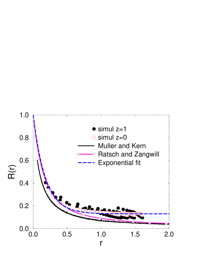
FIG. 2.: Shape factor $R(r)$ as a function of the aspect ratio $r$. The solid line has been obtained from the equation : $R(r)=0.13+0.87*\exp(-r/0.18)$. We have also compared our simulations with the predictions of Kern and Müller and Ratsch and Zangwill.

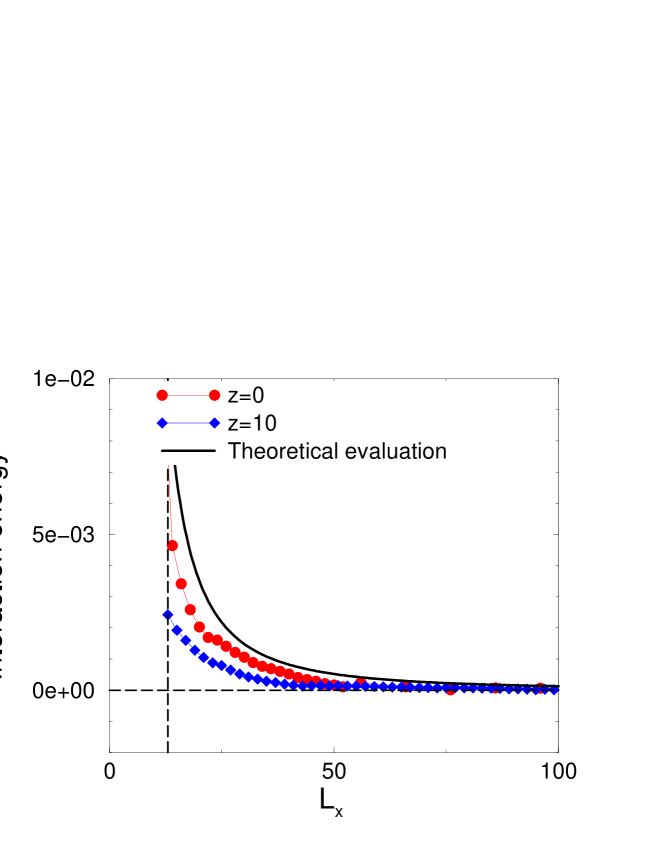
FIG. 3.: Interaction Energy between two islands as a function of the distance between islands. We have drawn two curves obtained by simulations for different heights of the wetting layer ($z=0$ and $z=10$), and the curve obtained from Eq. 12 without any adjustable parameter. The vertical dashed line corresponds to the two islands touching. Values of $n_{sub}$ used for the calculation of the curve are $n_{sub}=240$ for $z=0$ and $n_{sub}=90$ for $z=10$.

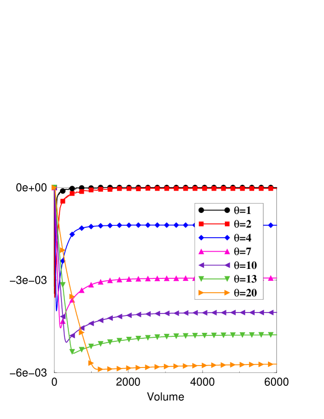
FIG. 4.: Variation of Energy per particle as a function of the volume for a given value of the coverage $\theta$. For each curve, only one point out of 50 has been precised in an aim to keep the figure clear.

FIG. 5.: Variation of the volume of the islands and of the distance between islands at the minimum of energy as a function of the coverage $\theta$.

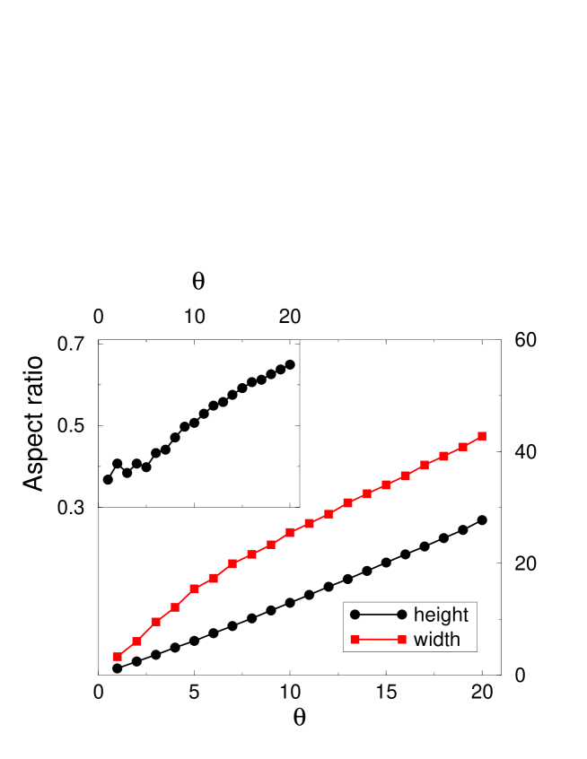
FIG. 6.: Variation of the island height and width at the minimum of energy as a function of the coverage $\theta$. In the inset, we plot the corresponding island aspect ratio as a function of $\theta$.

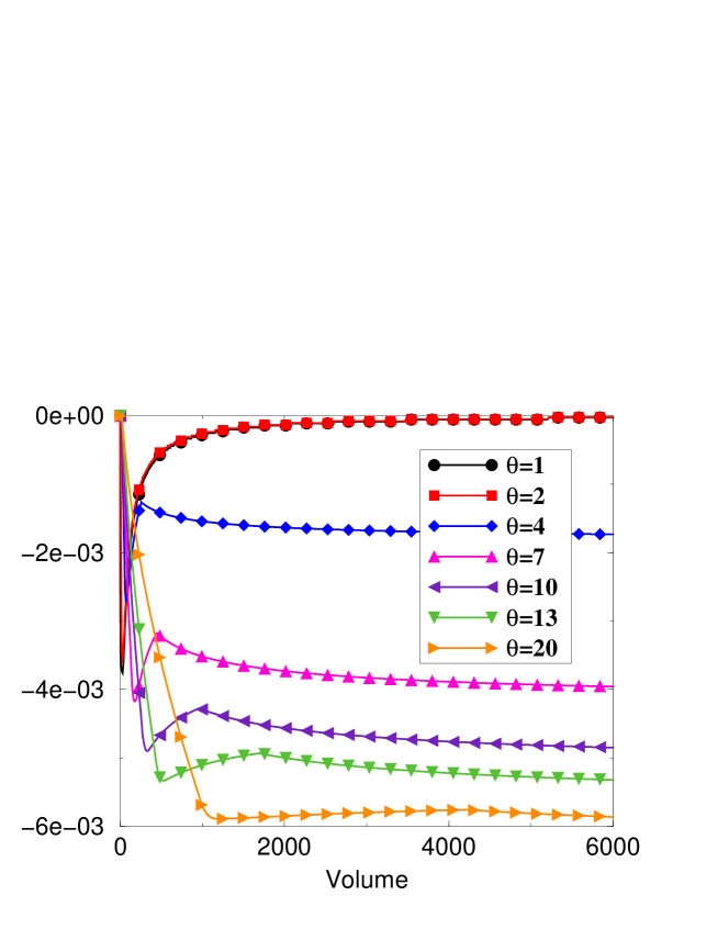
FIG. 7.: Variation of Energy per particle as a function of the volume for a given value of the coverage $\theta$ with $S(z)$ given by Eq. 31 and 32. For each curve, only one point out of 50 has been precised in an aim to keep the figure clear.

REFERENCES

- [1] B. G. Levi, Phys. Today 46 (1996) 22.
- [2] P. Venezuela, J. Tersoff, J. A. Floro, E. Chason, D. M. Follstaedt, F. Liu, and M. G. Lagally, Nature 397 (1999) 678.
- [3] S. Guha, A. Madhukar, and K. C. Rajkumar, Appl. Phys. Lett. 57 (1990) 2110.
- [4] Y. W. Mo, E. Savage, B. S. Swartzentruber, and M. G. Lagally, phys. Rev. Lett. 65 (1990) 1020.
- [5] R. Loo, D. Dentel, M. Goryll, P. Meunier-Beillard, D. Vanhaeren, L. Vescan, H. Bender, M. Caymax, and W. Vandervorst, J. Appl. Phys. (2001), accepted.
- [6] J. Tersoff and R. M. Tromp, Phys. Rev. Lett. 70 (1993) 2782.
- [7] V. A. Shchukin and D. Bimberg, Rev. Mod. Phys. 71 (1999) 1125.
- [8] M. A. Grinfeld, Dolk. Acad. Nauk SSSR 290 (1986) 1358, [Sov. Phys. Dolk. 31 (1986) 831].
- [9] D. J. Srolovitz, Acta metall. 37 (1989) 621.
- [10] B. J. Spencer, P. W. Voorhees, and S. H. Davis, Phys. Rev. Lett. 67 (1991) 3696.
- [11] F. M. Ross, R. M. Tromp, and M. C. Reuter, Science 286 (1999) 1931.
- [12] C. Priester and M. Lannoo, Phys. Rev. Lett. 75 (1995) 93.
- [13] L. G. Wang, P. Kratzer, M. Scheffler, and N. Moll, phys. Rev. Lett. 82 (1999) 4042.
- [14] P. R. Kratzer, M. Rabe, and F. Henneberger, Phys. Rev. Lett. 83 (1999) 239.
- [15] V. A. Shchukin, N. N. Ledentsov, P. S. Kop’ev, and D. Bimberg, Phys. Rev. Lett. 75 (1995) 2968.
- [16] J. Tersoff and F. K. Legoues, Phys. Rev. Lett. 72 (1994) 3570.
- [17] L. D. Landau and E. M. Lifshitz, Theory of elasticity (Pergamon Press, Oxford, 1986).
- [18] R. Kern and P. Müller, Surf. Sci. 392 (1997) 103.
- [19] P. Müller and R. Kern, J. Crystal Growth 193 (1998) 257.
- [20] C. Ratsch and A. Zangwill, Surf. Sci. 293 (1993) 123.
- [21] D. Wong and M. D. Thouless, J. Mater. Sci. 32 (1997) 1835.
- [22] P. Müller and R. Kern, Microsc. Microanal. Microstruct. 8 (1997) 229.
- [23] P. Müller and O. Thomas, Surf. Sci. 465 (2000) L764.
- [24] R. A. Bennett, S. Poulson, N. J. Price, J. P. Reilly, P. Stone, C. J. Barnes and M. Bowker, Surf. Sci. 433-435 (1999) 816.
- [25] M. PhanerGoutorbe, Y. Robach, P. Krapf, A. Solere, and L. Porte, Surf. Sci. 404 (1998) 268.
- [26] F. M. Ross, J. Tersoff, and R. M. Tromp, Phys. Rev. Lett. 80 (1998) 984.
- [27] J. Tersoff, Phys. Rev. B 39 (1998) 5566.
a)
b)