Impurity band in clean superconducting weak links

Abstract

Weak impurity scattering produces a narrow band with a finite density of states near the phase difference $\phi=\pi$ in the mid-gap energy spectrum of a macroscopic superconducting weak link. The equivalent distribution of transmission coefficients of various conducting quantum channels is found.

Effect of impurities on transport properties of superconducting nanostructures is one of the key issues in the physics of mesoscopic superconductors (see Beenakker/rev for a review). Recent advances in nanotechnology revived interest in quantum point contacts (see Lodder and references therein) and in other devices that employ quantum conductors connected to superconducting electrodes Pierre . SNS junctions and weak links consisting of two superconductors connected by a small orifice in a thin insulating layer (point contacts) are the simplest devices of interest. Though impurity effects in SNS junctions are well studied (the work began with Ref. Mitsai and still goes on, see for example Zhou ), the role of impurity scattering in superconducting point contacts remains not fully investigated.

As an example, consider a ballistic point contact between two superconductors assuming that the thickness $d$ of the insulating layer and the size of the orifice $a$ are shorter than the coherence length $\xi$ and the impurity mean free path $\ell$. As is well known Kulik ; KulikOmel there exist mid-gap states with the spectrum

$$\epsilon=\pm\epsilon_{0},\;\epsilon_{0}=|\Delta|\cos(\phi/2)$$ (1)

Here $\phi=\chi_{2}-\chi_{1}$, with $\chi_{1,2}$ being the order parameter phase on the left (right) from the orifice; the upper sign refers to particles moving to the right from region 1 into region 2 and vice versa. Impurities do not appear in Eq. (1) because the characteristic dimension is determined by the size of the constriction $d$ rather than by $\xi$, the parameter $d/\ell$ being assumed infinitely small. It is natural to expect however that the impurity scattering would modify this spectrum at an energy scale determined by the small parameter $d/\ell$, especially for low energies where the two branches of the spectrum for right- and left-moving particles cross. The same can be expected for a long ballistic SNS junction which has a mid-gap spectrum Mitsai ; Kulik consisting of many branches for right- and left-moving particles that cross at $\phi=\pi$.

In this Letter we consider both point contacts and long SNS junctions and show that a weak impurity scattering transforms their mid-gap spectra in such a way that a narrow band having a finite density of states and a width $\sim|\Delta|\sqrt{d/\ell}$ appears near each crossing point at the phase difference $\phi=\pi$. This impurity band is expected to have a dramatic effect on dynamic properties of weak links. In particular, it enhances the inelastic electron-phonon relaxation rate at low temperatures which would be otherwise nearly zero due to the energy conservation.

Impurity band in a point contact.–We consider first a ballistic point contact such that $a\sim d\ll\xi\ll\ell$. One has $\Delta_{1,2}=|\Delta|e^{i\chi_{1,2}}$ to the left (right) from the orifice, respectively (see Fig. 1 ). The quasiclassical Green functions (retarded or advanced) satisfy the normalization $g^{2}-ff^{\dagger}=1$ and obey the Eilenberger equations Eilenberger

$$-iv_{F}\frac{\partial g}{\partial s} = \frac{i}{2\tau}\left(f\left\langle f^{\dagger}\right\rangle-\left\langle f\right\rangle f^{\dagger}\right)$$ (2)

$$-iv_{F}\frac{\partial f}{\partial s}-2\epsilon f+2\Delta g = \frac{i}{\tau}\left(\left\langle g\right\rangle f-\left\langle f\right\rangle g\right),$$ (3)

$$iv_{F}\frac{\partial f^{\dagger}}{\partial s}-2\epsilon f^{\dagger}+2\Delta^{*}g = \frac{i}{\tau}\left(\left\langle g\right\rangle f^{\dagger}-\left\langle f^{\dagger}\right\rangle g\right)$$ (4)

where $s$ is the distance along the particle trajectory. We assume zero magnetic field. The right-hand sides of these equations describe the scattering by impurities. We use $\langle\ldots\rangle$ to denote an average over the Fermi surface. The standard technique of averaging over impurities is applicable because the number of impurities within the volume of the orifice is large. Indeed, the mean free time is $\tau^{-1}\sim N_{F}n_{{\rm imp}}|u|^{2}$ where $|u|\sim Up_{F}^{-3}$ is the Fourier transform of the impurity potential $U$, and $N_{F}$ is the normal single-spin density of states at the Fermi level. The number of impurities $n_{{\rm imp}}da^{2}\sim(d/\ell)(p_{F}a)^{2}(E_{F}/U)^{2}$ can be very large even for $U\sim E_{F}$ because of a macroscopic number of quantum channels in the orifice $(p_{F}a)^{2}\gg 1$.

For low energies $|\epsilon|\ll|\Delta|$ and close to $\phi=\pi$ the Green functions are localized near the orifice at distances $s\sim\xi$. We put $\phi=\pi+\delta$ where $\delta\ll 1$ so that $\Delta_{1}=-i|\Delta|e^{-i\delta/2},\;\Delta_{2}=i|\Delta|e^{i\delta/2}$. Following KrPe we write

$$f_{\pm}=\mp i\zeta_{\pm}\pm\eta_{\pm},\;f^{\dagger}_{\pm}=\mp i\zeta_{\pm}\mp\eta_{\pm}.$$ (5)

The upper sign is for right-moving particles, $p_{x}>0$, the lower sign is for left-moving particles, $p_{x}<0$. The $x$ axis is perpendicular to the insulating layer. We assume $\zeta^{2}\gg 1-\eta^{2}$ so that $g_{\pm}=i\zeta_{\pm}$. Equations (3, 4) become

$$v_{F}\frac{\partial\zeta_{\pm}}{\partial s}+2\zeta_{\pm}|\Delta|\cos(\delta/2){\rm sign}(s)=0,$$

$$v_{F}\frac{\partial\eta_{\pm}}{\partial s}-\left(2\epsilon\mp 2|\Delta|\sin(\delta/2)+i\sigma_{\pm}\right)\zeta_{\pm}=0,$$

where

$$\sigma_{\pm}=\tau^{-1}\left(\left\langle g\right\rangle\pm\left\langle f\right\rangle/2\pm\left\langle f^{\dagger}\right\rangle/2\right).$$ (6)

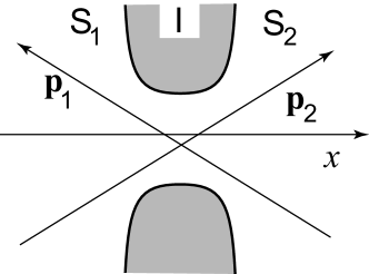
Figure 1: The point contact between two superconductors ($S_{1}$ and $S_{2}$) separated by an insulating layer (I). The $x$ axis is directed from the region where the order parameter phase is $\chi_{1}$ into the region where the phase is $\chi_{2}$.

The boundary conditions for $s\rightarrow\infty$ follow from the expressions for the Green functions in the bulk. For small $\delta$, the functions $\zeta_{\pm}\rightarrow 0$ and $\eta_{\pm}\rightarrow 1$. The solution is

$$\zeta_{\pm} = C_{\pm}\exp\left(-K\right),\;K=2|\Delta||s|/v_{F},$$

$$\eta_{\pm} = C_{\pm}v_{F}^{-1}\int_{0}^{s}e^{-K}\left(2|\Delta|E_{\pm}+i\sigma_{\pm}\right)\,ds,$$

$$C_{\pm} = \left[E_{\pm}+iv_{F}^{-1}\int_{0}^{\infty}\sigma_{\pm}\,ds\right]^{-1}.$$

Here $E_{\pm}=\epsilon/|\Delta|\mp\sin(\delta/2)$.

The averages $\left\langle g\right\rangle$, etc., are proportional to the solid angle at which the orifice is visible from the position point, they decrease quickly at distances $s\sim a$ from the orifice. Indeed, $g\left({\bf p},{\bf r}\right)=\mp f\left({\bf p},{\bf r}\right)=i\zeta\left(0\right)$ for trajectories that go through the orifice and $g\left({\bf p},{\bf r}\right)=f\left({\bf p},{\bf r}\right)=0$ otherwise because, for non-through trajectories, the Green functions are small as compared to $\zeta\gg 1$. For $s\sim a$ one has $K=0$. Moreover, using Eq. (5) we find

$$v_{F}^{-1}\int\sigma_{\pm}\,ds=\ell^{-1}\int ds\left\langle g(0)\right\rangle_{\mp}=\gamma g_{\mp}(0)$$

where $\left\langle g\right\rangle_{\pm}=(2\pi)^{-1}\int_{\pm p_{x}>0}g({\bf p},{\bf r})\,d\Omega_{{\bf p}}$, and $\gamma\sim d/\ell$ is a geometric factor depending on the shape of the contact and on the position of the trajectory with respect to the orifice. We neglect the latter dependence and consider a constant $\gamma$ for simplicity. Finally,

$$g_{\pm}^{R(A)}\left(s\right)=ie^{-K}\left[E_{\pm}+i\gamma g_{\mp}^{R(A)}\left(0\right)\right]^{-1}.$$ (7)

In the limit $\gamma\rightarrow 0$, the Green functions have poles at $E_{\pm}=0$ which is Eq. (1). The spectrum is shown in Fig. 2 by lines (1) for $p_{x}>0$ and (2) for $p_{x}<0$. However, as $E_{+}E_{-}$ approaches $\gamma$, the apparent pole-like behavior of Eq. (7) transforms into a more complicated dependence. To calculate the Green functions, we solve Eq. (7) for $g_{\pm}(0)$. If $0<E_{+}E_{-}<4\gamma$, i.e.,

$$\sin^{2}(\delta/2)<\epsilon^{2}/|\Delta|^{2}<4\gamma+\sin^{2}(\delta/2)$$ (8)

we find $g_{\pm}^{R}\left(s\right)=g_{\pm}^{R}\left(0\right)e^{-K}$ where

$$g_{\pm}^{R}\left(0\right)=\frac{E_{\mp}}{2\gamma}\left(i+\sqrt{\frac{4\gamma}{E_{+}E_{-}}-1}\right),$$ (9)

and $g^{A}=-[g^{R}]^{*}$. The radical is defined as an analytical function with the cuts along the borders of the region determined by Eq. (8) (shaded region in Fig. 2). The sign is chosen for $\epsilon$ within the upper part of the region. The normalized density of states $\nu_{\epsilon}(s)=\left[g^{R}\left(s\right)-g^{A}\left(s\right)\right]/2$ is nonzero within the energy interval of Eq. (8). The maximum half-width of the energy band $2\sqrt{\gamma}$ is reached for $\delta=0$. Inside the constriction

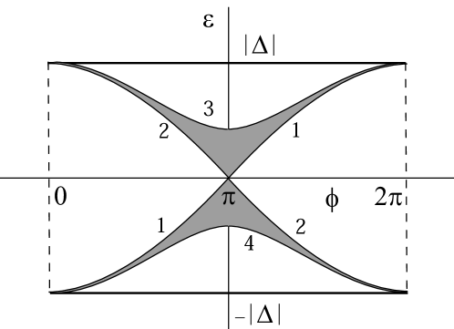
Figure 2: Lines 1, 2, 3, and 4 encompass the energy band with a finite density of states (shaded region). The maximum half-width of the band is $2\sqrt{\gamma}$. For a ballistic contact $\tau\rightarrow\infty$, the spectrum is given by Eq. (1) and follows lines 1 and 2. The entire pattern is $2\pi$-periodic in $\phi$.

$$\nu_{\epsilon\pm}(0)=\frac{E_{\mp}}{2\gamma}\sqrt{\frac{4\gamma}{E_{+}E_{-}}-1}$$ (10)

For a particle with a given sign of $p_{x}$ the density of states is nonzero near both $E_{-}=0$ and $E_{+}=0$: the scattering mixes states with positive and negative $p_{x}$. However, far from the crossing point, $|\epsilon|\gg|\Delta|\sqrt{\gamma}$, the ratio $\nu_{\pm}/\nu_{\mp}=E_{\mp}/E_{\pm}$ is large near the corresponding ballistic spectrum $E_{\pm}=0$: its magnitude is of the order $\epsilon^{2}/|\Delta|^{2}\gamma$.

Beyond the range of Eq. (8) $g^{R}$ and $g^{A}$ coincide and the density of states vanishes. For $E_{+}E_{-}>4\gamma$,

$$g_{\pm}^{R}(0)=g_{\pm}^{A}(0)=\frac{iE_{\mp}}{2\gamma}\left(1-\sqrt{1-\frac{4\gamma}{E_{+}E_{-}}}\right).$$

For $\gamma\ll|E_{+}E_{-}|$ one recovers the poles $g_{\pm}^{R(A)}\left(0\right)=i/E_{\pm}$ with the density of states $\nu=\pi|\Delta|\delta(\epsilon\mp\epsilon_{0})$. Obviously, Eq. (10) conserves the total number of states since $\int\nu_{\pm}\,d\epsilon=\pi|\Delta|$ for any $\phi$.

Long SNS bridge.– Consider now a normal bridge of a length $d\gg\xi$ that connects two massive superconductors. Its width is much shorter than $\xi$. We assume that it has specular walls. Irregularities on the walls can also be modelled by random impurities. Superconductors and the normal metal have the same Fermi velocities $v_{F}$. We take the $x$ axis along the bridge (see Fig. 3).

Figure 3: Normal bridge between two bulk superconductors.

Let $s=\pm s_{0}=\pm d/|\cos\theta|$ be the outlets of the normal bridge into the bulk superconductors. For $s<-s_{0}$ the solutions in the bulk are Mitsai ; Kulik

$$g_{\pm}=g_{\infty}+g_{\pm k}e^{k(s+s_{0})},~{}f_{\pm}=f_{\infty}+g_{\pm k}\beta_{k}e^{k(s+s_{0})}$$ (11)

where $f_{\infty}=\Delta/i\sqrt{|\Delta|^{2}-\epsilon^{2}}$, $g_{\infty}=\epsilon/i\sqrt{|\Delta|^{2}-\epsilon^{2}}$ while $k=2v_{F}^{-1}\sqrt{\left|\Delta\right|^{2}-\epsilon^{2}}$ and $\beta_{k}=\Delta/\left(\epsilon+iv_{F}k/2\right)$. The impurity scattering in the bulk can be neglected. The signs correspond to $\pm p_{x}>0$; the order parameter phase should be $\chi_{1}$ for $p_{x}>0$ and $\chi_{2}$ for $p_{x}<0$. For $s>s_{0}$

$$g_{\pm}=g_{\infty}+g_{\pm k}e^{-k(s-s_{0})},~{}f_{\pm}=f_{\infty}+g_{\pm k}\beta_{-k}e^{-k(s-s_{0})}.$$ (12)

Here the phase is $\chi_{2}$ for $p_{x}>0$ and $\chi_{1}$ for $p_{x}<0$.

We first outline the known solution Mitsai ; Kulik for states with not very low energies $v_{F}/d\ll\epsilon$ such that $d\gg\xi_{N}$ Here $\xi_{N}\sim v_{F}/T$. In the region inside the bridge where $\Delta=0$ Eqs. (2–4) yield $g^{2}\equiv g^{2}_{N}=const$ and

$$f=C\exp\left[i\left(2\epsilon+\frac{i}{\tau}\left\langle g_{N}\right\rangle\right)\frac{x}{v_{x}}\right]$$

where $v_{x}=v_{F}\cos\theta$ and $x=s\cos\theta$. We assumed that $\left\langle f\right\rangle=\left\langle f^{\dagger}\right\rangle=0$. Indeed, $f$ and $f^{\dagger}$ oscillate rapidly as functions of $\theta$ since $\epsilon d/v_{F}\gg 1$ and vanish after averaging over the angles. The continuity at the borders between the bridge and the bulk gives $g_{\pm k}=g_{\pm N}-g_{\infty}$ and

$$g_{\pm N}=\frac{\tan\alpha\pm ig_{\infty}}{g_{\infty}\tan\alpha\pm i}$$ (13)

where $\alpha=(d/v_{x})\left(2\epsilon+i\left\langle g_{N}\right\rangle/\tau\right)-\phi/2$. For $\left|\epsilon\right|<\left|\Delta\right|$, the function $g_{\pm N}$ has poles when $\alpha=\pm\arccos\left(\epsilon/\left|\Delta\right|\right)+\pi n$ or Mitsai ; Kulik

$$\epsilon+\frac{i}{2\tau}\left\langle g_{N}\right\rangle=\pm\omega_{x}\left[\frac{\phi}{2}+\pi\left(n+\frac{1}{2}\right)-\arcsin\left(\frac{\epsilon}{|\Delta|}\right)\right]$$

where $\omega_{x}=|v_{x}|/2d$. The state with $n=-1$ has $\epsilon=0$ for $\phi=\pi$. The spectrum for $\tau=\infty$ is shown in Fig. 4 by lines 1 and 2. For $\epsilon\gg v_{F}/d$, the poles are closely packed. As a result, the angular average collects contributions from many poles which givesMitsai $\left\langle g_{N}^{R\left(A\right)}\right\rangle=\pm 1$.

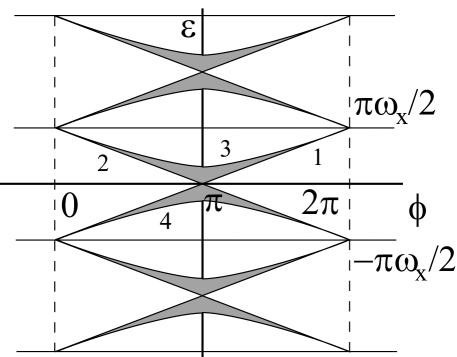
Figure 4: The energy bands (shaded regions) for a long SNS bridge. Lines 1 and 2 show the spectrum of a particle with $p_{x}>0$ and $p_{x}<0$, respectively, in a ballistic bridge $\ell\rightarrow\infty$. The pattern is $2\pi$-periodic in $\phi$.

For low energies $\epsilon\ll|\Delta|$, the term $g_{\infty}\tan\alpha\ll 1$ if $d\gg\xi$. Eq. (13) results in $g_{N}=\tan\alpha$. The Green function is large when $\alpha$ is close to $\pi/2+\pi n$, i.e., close to the points $\epsilon=\omega_{0}\pi m$ where the branches for $p_{x}>0$ and for $p_{x}<0$ cross. Consider these regions in more detail. We put $\epsilon=\epsilon^{\prime}+\omega_{0}\pi m$ and write the functions in the normal bridge as $f=\tilde{f}\exp(\pm i\pi mx/d)$, $f^{\dagger}={\tilde{f}}^{\dagger}\exp(\mp i\pi mx/d)$. We now express $\tilde{f}$ and ${\tilde{f}}^{\dagger}$ through $\eta$ and $\zeta$ according to Eq. (5) and assume $g_{N}=i\zeta$. The solution of Eqs. (3, 4) is $\zeta_{\pm}=A_{\pm}=const$ and

$$\eta_{\pm}=A_{\pm}v_{x}^{-1}\int_{0}^{x}\left(2\epsilon^{\prime}+i\sigma_{\pm}\right)\,dx.$$

Here $\sigma_{\pm}$ is determined by Eq. (6) where $f,\,f^{\dagger}$ are replaced with $\tilde{f},\,{\tilde{f}}^{\dagger}$. Note that now $K=0$. Matching this with Eqs. (11, 12) at $x=\pm d$ we obtain

$$g_{\pm N}=\frac{i\omega_{x}}{\epsilon^{\prime}+i\sigma_{\pm}/2\mp\omega_{x}\delta/2}$$ (14)

where $\phi=\pi+\delta$. Using Eq. (5) we find $\sigma_{\pm}=\left\langle g\right\rangle_{\mp}/\tau$.

The angle-resolved density of states is proportional to the averaged $g^{R}-g^{A}$. Calculating the average we obtain

$$\left\langle g_{N}\right\rangle_{\pm}=i\omega_{0}\int_{0}^{1}\frac{\mu\,d\mu}{\epsilon^{\prime}+i\left\langle g\right\rangle_{\mp}/2\tau\mp\mu\omega_{0}\delta/2}$$ (15)

where $\omega_{0}=v_{F}/2d$. We put $x=\delta/2\sqrt{\gamma},\;y=\epsilon^{\prime}/\omega_{0}\sqrt{\gamma},\;z_{\pm}=\sqrt{\gamma}\left\langle g_{N}\right\rangle_{\pm}$ where $\gamma=d/\ell$. Performing integration in Eq. (15) for $\delta\sim\sqrt{\gamma}$ and $\epsilon\sim\omega_{0}\sqrt{\gamma}$ we find

$$z_{\pm}=\mp\frac{i}{x}-\frac{i(y+iz_{\mp})}{x^{2}}\ln\left[\frac{y+iz_{\mp}\mp x}{y+iz_{\mp}}\right].$$ (16)

For small $x$ one has $z_{+}=z_{-}=\left[iy\pm\sqrt{2-y^{2}}\right]/2$ which is similar Eq. (9). For $y<\sqrt{2}$, the functions $\left\langle g^{R}\right\rangle=-\left\langle g^{A}\right\rangle^{*}$ are complex, thus the density of states is nonzero, $\left\langle\nu\right\rangle\sim 1/\sqrt{\gamma}$. For $y>\sqrt{2}$ solutions are imaginary, $\nu=0$. To find the limit where a nonzero density of states appears, we look for $z=ia$ and find conditions when there are no real solutions for $a$. We have

$$a_{\pm}=\mp\frac{1}{x}-\frac{y-a_{\mp}}{x^{2}}\ln\left[\frac{y-a_{\mp}\mp x}{y-a_{\mp}}\right].$$ (17)

For small $x$ we return to the previous result: the density of states vanishes for $y>\sqrt{2}$. However, if $\epsilon^{\prime}=y=0$ a real solution for $a$ exists for any $x$: the density of states is zero along the axis $\epsilon^{\prime}=0$ which agrees with Eq. (8). Next, we note that the density of states is singular at one of the borders of its region of existence. Thus, either $a_{+}$ or $a_{-}$ should go to infinity. Assume that $a_{+}\rightarrow\infty$. Then $a_{-}\rightarrow 0$ according to the second equation (17). In turn,

$$a_{+}=-\frac{1}{x}-\frac{y}{x^{2}}\ln\left[\frac{y-x}{y}\right].$$

Infinite values for $a_{+}$ are possible for $y=x$. Similarly, assuming $a_{-}\rightarrow\infty,\;a_{+}\rightarrow 0$ we finally find the borders of the region with a nonzero density of states, $y=\pm x$ or

$$|\epsilon^{\prime}|=\omega_{0}|\delta|/2.$$ (18)

Equation (18) gives the lower-$|\epsilon^{\prime}|$ limits shown in Fig. 4 by lines 1 and 2. The higher-energy limits (lines 3 and 4 in Fig. 4) are set by $|y|=\sqrt{2}$ for small $x$. For large $x$ and $y$ we expect that one of $a_{\pm}$ is large while the other is small. We then again obtain Eq. (18) as the asymptotic expression. Therefore, the two borders approach each other for large $x$ and $y$, as was also the case for a point contact. We thus expect that Eq. (10) provides a qualitatively correct representation for the averaged density of states of a long SNS junction, as well.

Discussion.–The results for point contacts and for long SNS bridges are qualitatively similar. To simplify the discussion we consider the impurity band in a point contact where an explicit equation for the density of states is available. It can be compared with the known mid-gap energy spectrumZaitsev ; Beenakker for a contact that has a tunnel barrier with a transmission probability $D$,

$$\epsilon=\pm\epsilon_{D},\;\epsilon_{D}=|\Delta|\sqrt{1-D\sin^{2}(\phi/2)}.$$ (19)

In Fig. 2 this spectrum follows lines (3) and (4) and has a gap with the half-width $|\Delta|\sqrt{R}$ at $\phi=\pi$ where $R=1-D$ is the reflection coefficient. The gap results from the mixing of right- and left-moving particles provided by the barrier. One can consider the impurity band Eq. (8) as a result of superposition of a large number of conduction channels with various transmission coefficients $D$ resulting from scattering of particles on different trajectories characterized by a given momentum. Superposition of states with different momenta due to scattering by impurities is also known to produce an impurity band in $d$-wave superconductors near the gap nodes GorkKal . To find the equivalent probability distribution $P(D)$ we write the total density of states for an energy $\epsilon$ in the form

$$\left\langle\nu\right\rangle_{+}+\left\langle\nu\right\rangle_{-}=\pi|\Delta|\int\left[\delta\left(\epsilon-\epsilon_{D}\right)+\delta\left(\epsilon+\epsilon_{D}\right)\right]P(D)\,dD.$$

The relevant values of $D$ are close to one. With help of Eqs. (10) and (19) we find

$$P(D)=\frac{1}{2\pi\gamma}\,\frac{\sqrt{4\gamma-R}}{\sqrt{R}},\;R<4\gamma.$$ (20)

The distribution is truncated at $R\geq 4\gamma$. For $\gamma\rightarrow 0$ one obtains $P(D)=\delta(R)$. The square-root singularity at $R=0$ in Eq. (20) resembles that of the universal distribution Dorokhov for diffusive normal conductors. The singularity ensures a finite density of states at $\phi=\pi$ which is $\nu=(1/\sqrt{\gamma})\sqrt{1-(\epsilon^{2}/4\gamma|\Delta|^{2})}$ according to Eq. (10). However, Eq. (20) is not universal: in contrast to its diffusive counterpart it depends on the geometry of the contact and on the quasiparticle mean free path.

The impurity band is expected to have a profound effect on dynamics of weak links. For example, it enhances the electron-phonon relaxation at low temperatures which otherwise would almost vanish due to the energy conservation. Indeed, the electron-phonon relaxation rate is proportional to the product of two electron densities of states $\nu_{\epsilon}$ and $\nu_{\epsilon_{1}}$, and the phonon density of states $N_{\rm ph}(\omega)$ where $\omega=\epsilon-\epsilon_{1}$. Since $N_{\rm ph}(\omega)\propto\omega^{2}$ the product vanishes if each electronic density of states is a delta function $\delta(\epsilon-\epsilon_{0})$ with only one state $\epsilon_{0}$ for a given phase $\phi$ and the sign of momentum $p_{x}$. It is the impurity scattering that broadens the density of states into a band thus making the electron-phonon relaxation possible.

I thank D. Averin, Yu. Barash, M. Feigel’man, and G. Volovik for instructive discussions. This work was supported by Russian Foundation for Basic Research.

References

(1) C. W. J. Beenakker, Rev. Mod. Phys. 69,
731 (1997).
(2) A. Lodder and Yu. V. Nazarov, Phys. Rev. B 58,
5783 (1998).
(3) F. Pierre, A. Anthore, H. Pothier, C. Urbina, and D. Esteve, Phys. Rev. Lett. 86, 1078 (2001).
(4) I. O. Kulik and Yu. N. Mitsai, Fiz. Nizk. Temp. 1, 906 (1975) [Sov. J. Low Temp. Phys. 1, 434 (1975)].
(5) F. Zhou and B. Spivak, Phys. Rev. Lett. 80, 5647
(1998).
(6) I. O. Kulik, Zh. Eksp. Teor. Fiz. 57, 1745 (1969)
[Sov. Phys. JETP 30, 944 (1970)].
(7) I. O. Kulik and A. N. Omel’yanchuk, Fiz. Nizk.
Temp. 3, 945 (1977) [Sov. J. Low Temp. Phys. 3, 459 (1977)].
(8) G. Eilenberger, Z. Phys. 214, 195 (1968).
(9) L. Kramer and W. Pesch, Z. Phys. 269, 59 (1974).
(10) W. Haberkorn, H. Knauer, and J. Richter, Phys. Status
Solidi, 47, K161 (1978); A. V. Zaitsev,
Zh. Eksp. Teor. Fiz. 86, 1742 (1984)
[Sov. Phys. JETP 59, 1015 (1984)].
(11) C. W. J. Beenakker, Phys. Rev. Lett. 67, 3836
(1991).
(12) L. P. Gor’kov and P. Kalugin, Pis’ma Zh. Eksp. Teor.
Fiz. 41, 208 (1985) [JETP Lett. 41, 253 (1985)].
(13) O. N. Dorokhov, Solid State Commun. 51, 381 (1984);
Yu. V. Nazarov, Phys. Rev. Lett. 73, 134 (1994).