Injected Power Fluctuations in Langevin Equation

Abstract

In this paper, we consider the Langevin equation from an unusual point of view, that is as an archetype for a dissipative system driven out of equilibrium by an external excitation. Using path integral method, we compute exactly the probability density function of the power (averaged over a time interval of length $\tau$) injected (and dissipated) by the random force into a Brownian particle driven by a Langevin equation. The resulting distribution, as well as the associated large deviation function, display strong asymmetry, whose origin is explained. Connections with the so-called “Fluctuation Theorem” are thereafter discussed. Finally, considering Langevin equations with a pinning potential, we show that the large deviation function associated with the injected power is completely insensitive to the presence of a potential.

Keywords: Fluctuation phenomena, random processes, noise and Brownian motion.

1 Introduction

Usually, works concerning out of equilibrium stationary systems deal with their local statistical properties, some assumptions of homogeneity and isotropy being reasonably assumed or understood: traditional theory of turbulence, which focuses on local correlations of the velocity field furnishes a good illustration of that. A rather new way to study such systems was recently proposed by some authors [1, 2, 3], who preferred concentrate their efforts to characterize the process of injection of energy, imperatively required to sustain the stationary state. To be more precise, in numbers of such situations, there exists a channel of energy injection, usually located at boundaries of the system (rotating blades driving a turbulent flow, heated plate in Rayleigh-Bénard convection, piston shaking granular matter at an edge of a vessel, etc…) together with a distinct channel of dissipation, often provided by a bulk dissipation mechanism, viscosity or inelastic collisions. This duality is explicitly expressed in the dynamical equation for the energy which can always be written in the form $\dot{E}=\mathcal{I}-\mathcal{D}$, where $\mathcal{D}$ is proportional to a coefficient of dissipation whereas $\mathcal{I}$ is entirely due to the injection process: for instance, the evolution of the kinetic energy of an uncompressible fluid is given by

$$\partial_{t}\left[\rho\int_{V}\mathbf{v}^{2}dV\right]=\int_{\partial V}(\eta v_{i}\sigma_{ij}n_{j}-(p+\rho\mathbf{v}^{2}/2)\mathbf{v.n})dS-\frac{\eta}{2}\int_{V}\sigma_{ij}\sigma_{ij}dV,$$ (1)

where one recognizes easily a surface injection term and a dissipative bulk term ($\sigma_{ij}=\partial_{i}v_{j}+\partial_{j}v_{i}$) . These two distinct “gates” lead to the establishment of a permanent flow of energy throughout the system, and is obviously a primordial feature amongst the stationary properties of the system. Thus, some experimental measurements [1, 2, 3] and numerical simulations [4] were performed to characterize the injection of energy (more easily reachable than the dissipation), or more precisely the probability density function (pdf) $\pi(\varepsilon)$ of $\varepsilon=\frac{1}{\tau}\int_{0}^{\tau}\mathcal{I}(t)dt$, the averaged injected power during a time interval of length $\tau$. In particular, in some works [4, 5, 6], the quantity

$$\rho(\varepsilon)=\frac{1}{\tau}\log\frac{\pi(\varepsilon)}{\pi(-\varepsilon)}$$ (2)

was measured, and it was noticed that, according to the conclusions of the so-called “Fluctuation Theorem” [7, 8], $\rho(\varepsilon)$ seemed to tend to a straight line for large $\tau$. These observations were quite surprising, for the Fluctuation Theorem was established for time-reversal systems, a property which is at the heart of the demonstration of the theorem. A convincing argument was recently proposed [4] to explain this seemingly universal behaviour: if one considers that the signal of $\mathcal{I}(t)$ has only finite correlations, large deviation theory predicts that $\log\pi(\varepsilon)\sim\tau f(\varepsilon)$ for large $\tau$. Consequently, $\rho(\varepsilon)=f(\varepsilon)-f(-\varepsilon)$; but for large $\tau$, it is extremely unprobable to observe large negative occurences of the averaged injected power (but not unpossible), since in average, the injected power in a dissipative system is positive. As a result, in concrete measurements of $\rho(\varepsilon)$, one can presumably only measure $\rho$ in a short vicinity of zero, for which $f(\varepsilon)-f(-\varepsilon)\approx 2f^{\prime}(0)\varepsilon$ with an excellent approximation: that is why a straight line behaviour is always measured in real or numerical experiments.

Nevertheless, there was a lack of a real example of a nonequilibrium dissipative model in which $\pi(\varepsilon)$ could be fully computed, in order to show that time-reversal symmetry is absolutely required for the Fluctuation Theorem “really” to hold. The initial aim of this paper was thus to provide a simple model, where the pdf $\pi(\varepsilon)$ is exactly computable, and which mimics as simply as possible the presence of two distinct channels for energy flow. One of the simplest (nontrivial) systems fulfilling these requirements is provided by the Langevin equation

$$\dot{v}+\gamma v =\psi(t)$$ (3)

$$<\psi(t)\psi(t^{\prime})> =2D\delta(t-t^{\prime})$$ (4)

where fluctuations $\psi(t)$ and dissipation $\gamma v$ are considered as two different sources of modification of energy :

$$\frac{d}{dt}\left(\frac{1}{2}v^{2}\right) =\underbrace{-\gamma v^{2}}_{\mbox{dissipation}}+\underbrace{\psi v}_{\mbox{injection}}$$ (5)

Note that in absence of $\psi$, the system is clearly dissipative and non time-reversal invariant, a property also shared by realistic hydrodynamic or granular systems.

This interpretation of the Langevin equation is clearly uncommon: deriving the Langevin equation as an evolution equation for a Brownian particle in a thermalized surroundings, it appears clearly that the dissipative term $-\gamma v$ and the fluctuating term $\psi$ are two different faces of the action of the reservoir on the particle; the fluctuation-dissipation relation $D=\gamma k_{B}T$ testifies this profund link. In the present case however, we consider the Langevin equation as a given evolution equation, irrespective of its physical origin, and interpret it as a dissipative system $\dot{v}+\gamma v=0$ shaked by a random gaussian force $\psi$; in particular, we will make in the following no reference to the fluctuation-dissipation relation just cited.

Thus, we compute in this paper the pdf of

$$\varepsilon=\frac{1}{\tau}\int_{0}^{\tau}dt^{\prime}\psi(t^{\prime})v(t^{\prime})$$ (6)

in the permanent regime using the path integral method (we compute also the pdf of the dissipated power). We show as expected that the function $\rho(\varepsilon)$ is in this case not a straight line (to prevent any confusion, it is worth noting that our result is not contradictory with that of Kurchan [9], who proved the Fluctuation Theorem for the power injected by an external operator acting on a Brownian particle: the physical situation considered here is by no means the same), though this nonlinear behaviour is extremely difficult to verify numerically.

But some other interesting and novel features emerge also from our study, which concern merely the large deviation function $f(\varepsilon)$ associated with $\pi(\varepsilon)$: we show that this function is not a regular function but displays a unexpected second order singularity; we discuss its physical origin and show that it is intimately associated with the permanent regime which allows rare initial fluctuations of the velocity which have deep consequences for the large deviation function.

Finally, we study also the effect of a pinning potential on this large deviation function and show that adding a potential does not have rigorously any consequence on the large deviation function. This “universality” confirms the relevance of considering the averaged injected power as a probe for extracting global features of energy flow into a nonequilibrium system.

2 Free Brownian motion

2.1 Characteristic functions

We consider a particle of mass $1$, velocity $v$, whose dynamics is given by (3), and want to compute the pdf of $\varepsilon$ in the permanent regime. To do that it is convenient to compute first its characteristic function

$$\widehat{\pi}(\lambda)=\left\langle e^{-\lambda\tau\varepsilon}\right\rangle$$ (7)

which is related to the Fourier transform of $\pi(\varepsilon)$ by $FT[\pi(\varepsilon)](k)=\widehat{\pi}(-ik/\tau)$. In some works [10], one computes already at this stage the asymptotic exponential dependence of the characteristic function: $\langle e^{-\lambda\tau\varepsilon}\rangle\sim e^{\tau g(\lambda)}$, and retrieves $f(\varepsilon)$ as the inverse Legendre transform of $g(\lambda)$: $f(\varepsilon)=g(\lambda)+\lambda\varepsilon,\ \ g^{\prime}(\lambda)=-\varepsilon$. We will see that this procedure is not appropriate here, for reasons which will be made clear later. One prefers thus compute first exactly $\widehat{\pi}(\lambda)$, what is here fortunately feasible.

Let us consider the stochastic equation (3). The propagator $P(v_{1},\tau|v_{0},0)$ can be easily expressed in terms of a path integral [11, 12, 13]:

$$P(v_{1},\tau|v_{0},0)=e^{\frac{\gamma}{2}\tau}\times\int_{v(0)=v_{0}}^{v(\tau)=v_{1}}[\mathcal{D}v]\exp\left(-\frac{1}{4D}\int_{0}^{\tau}dt\left(\dot{v}+\gamma v\right)^{2}\right)$$ (8)

From this formula, one can deduce the probability density associated with a given path:

$$\mathcal{P}([v(u),0\leqslant u\leqslant\tau])=\exp\left(\frac{\gamma\tau}{2}-\frac{1}{4D}\int_{0}^{\tau}dt\left(\dot{v}+\gamma v\right)^{2}\right)$$ (9)

As a result, one has

$$\widehat{\pi}_{v_{0}}(\lambda) \equiv\left\langle e^{-\lambda\tau\varepsilon}\right\rangle_{v_{0}}=\int_{-\infty}^{\infty}dv_{1}\int_{v(0)=v_{0}}^{v(\tau)=v_{1}}[\mathcal{D}v]\mathcal{P}([v])\exp\left(-\lambda\int_{0}^{\tau}v(\dot{v}+\gamma v)\right)$$ (10)

$$=e^{\frac{\gamma\tau}{2}}\int_{-\infty}^{\infty}\!\!\!\!\!dv_{1}e^{-\left(\frac{\lambda}{2}+\frac{\gamma}{4D}\right)(v_{1}^{2}-v_{0}^{2})}\int_{v(0)=v_{0}}^{v(\tau)=v_{1}}\!\!\!\!\!\!\![\mathcal{D}v]\exp\left(-\frac{1}{4D}\int_{0}^{\tau}[\dot{v}^{2}+(\gamma^{2}+4D\lambda\gamma)v^{2}]\right)$$ (11)

where $\langle\ldots\rangle_{v_{0}}$ designates an average over the realizations of $v$ such that $v(0)=v_{0}$. The path integral in (11) is well-known and its value can be exactly computed [11]:

$$\int_{v(0)=v_{0}}^{v(\tau)=v_{1}}\!\!\!\!\!\!\![\mathcal{D}v]\exp\left(-\frac{1}{4D}\int_{0}^{\tau}[\dot{v}^{2}+\alpha^{2}v^{2}]\right)=\\ \left(\pi\frac{4D}{\alpha}\sinh\alpha\tau\right)^{-1/2}\exp\left(-\frac{\alpha}{4D}\frac{(v_{1}^{2}+v_{0}^{2})\cosh(\alpha\tau)-2v_{0}v_{1}}{\sinh\alpha\tau}\right)$$ (12)

Thus, let us define

$$\widetilde{\gamma} =\gamma\tau$$ (13)

$$\widetilde{\lambda} =2D\lambda/\gamma$$ (14)

$$\eta =\sqrt{1+2\widetilde{\lambda}}$$ (15)

one has

$$\widehat{\pi}_{v_{0}}(\lambda) =e^{\widetilde{\gamma}/2}\left(\cosh\eta\widetilde{\gamma}+\frac{1+\widetilde{\lambda}}{\eta}\sinh\eta\widetilde{\gamma}\right)^{-1/2}\times\exp\left(\frac{v_{0}^{2}\gamma}{2D}\frac{\widetilde{\lambda}^{2}/2}{\eta\coth\eta\widetilde{\gamma}+1+\widetilde{\lambda}}\right)$$ (16)

To get $\widehat{\pi}(\lambda)$, one has to average over $v_{0}$ with a probability $\propto\exp(-v_{0}^{2}\gamma/2D)$, since it is the distribution of $v(t)$ in the permanent regime:

$$\widehat{\pi}(\lambda) =\sqrt{\frac{\gamma}{2D\pi}}\int dv_{0}\ e^{-v_{0}^{2}\gamma/2D}\left\langle e^{-\lambda\tau\varepsilon}\right\rangle_{v_{0}}$$ (17)

$$=e^{\widetilde{\gamma}/2}\left(\cosh\eta\widetilde{\gamma}+\frac{1+\widetilde{\lambda}-\widetilde{\lambda}^{2}/2}{\eta}\sinh\eta\widetilde{\gamma}\right)^{-1/2}$$ (18)

The calculation leading to (16) and (18) assumes a priori $\lambda>0$, but it is useful to study the properties of the analytical continuations of these formulae. First, one remarks that the square root in the definition of $\eta$ does not induce any breaking of analyticity, for it appears always in quantities such $\cosh(\eta\widetilde{\gamma})$ or $\sinh(\eta\widetilde{\gamma})/\eta$ which are entire functions of $\lambda$. Thus, one will assume in the following that $\eta=x+iy$ has positive real part.

Let us first look at $\widehat{\pi}_{v_{0}}(\lambda)$ for $v_{0}=0$ (the exponential term will not modify the analytical properties of $\widehat{\pi}_{v_{0}}(\lambda)$). It is astute to write it as

$$\left\langle e^{-\lambda\tau\varepsilon}\right\rangle_{0} =e^{(1-\eta)\widetilde{\gamma}/2}\left(\frac{1+e^{-2\eta\widetilde{\gamma}}}{2}\right)^{-1/2}\times\left(1+\frac{1}{2}\left(\eta+\frac{1}{\eta}\right)\tanh\eta\widetilde{\gamma}\right)^{-1/2}$$ (19)

and assume again a cut in the negative real semi-axis for the definition of the square root. Breaks in analyticity can arise if only one of the two terms of (19) (separated by “$\times$”) is not defined (a superposition of two cuts restores the analyticity, since they are associated with a square root). The last term is not defined for $\eta=x+iy$ such that

$$x=0\ \ \text{and}\ \ 1<\frac{1}{2}\left(y-\frac{1}{y}\right)\tan\widetilde{\gamma}y$$ (20)

This induces in the $\widetilde{\lambda}$-space a dashed half cut localized in the negative real axis, beginning at the value $\widetilde{\lambda}_{-}$ of $\widetilde{\lambda}$ less but closest to $-\frac{1}{2}$ such that

$$1=\frac{1}{2}\left(\sqrt{|1+2\widetilde{\lambda}_{-}|}-\frac{1}{\sqrt{|1+2\widetilde{\lambda}_{-}|}}\right)\tan\widetilde{\gamma}\sqrt{|1+2\widetilde{\lambda}_{-}|}$$ (21)

As $\widetilde{\gamma}\propto\tau$, it is clear that $\widetilde{\lambda}_{-}\rightarrow-\frac{1}{2}$ when $\tau\rightarrow\infty$.

The first term $e^{(1-\eta)\widetilde{\gamma}/2}\sqrt{2/(1+e^{-2\eta\widetilde{\gamma}})}$ , as a function of $\eta$, is analytical in the region $x\geqslant 0$ (except at points $x=0,y\equiv\frac{\pi}{2}[\pi]$). But if one considers it now as a function of $\widetilde{\lambda}$, it appears cuts in the $\widetilde{\lambda}$-space due to the prescription $x=\text{Re}(\eta)>0$. It is easy to verify that these cuts are defined by

$$(1+2\widetilde{\lambda})\in\frac{1}{\widetilde{\gamma}}[-(3\pi/2+2k\pi)^{2},-(\pi/2+2k\pi)^{2}],\ \ \text{for $k\in{\mathbb{N}}$}$$ (22)

and again are located in the $\widetilde{\lambda}<-\frac{1}{2}$ half axis.

To summarize, $\widehat{\pi}_{v_{0}}(\lambda)$ continued on the whole complex plane (as a function of $\lambda$) has a cut, dashed line shaped and localized on the negative real axis. It begins at a value $\widetilde{\lambda}_{-}$ less than $-\frac{1}{2}$, but tends to $-\frac{1}{2}$ for large $\tau$.

For $\widehat{\pi}(\lambda)$, the situation is similar, and gives also this dashed negative cut. But there is a fundamental discrepancy, for the “second term” $[1+(1+\widetilde{\lambda}-\widetilde{\lambda}^{2}/2)\tanh(\eta\widetilde{\gamma})/2\eta]^{-1/2}$ gives here a novel cut, plain and localized on the positive real axis, and beginning at a value $\widetilde{\lambda}_{+}$ solution of

$$\left(\left[\sqrt{1+2\widetilde{\lambda}_{+}}\right]^{3}-6\sqrt{1+2\widetilde{\lambda}_{+}}-\frac{3}{\sqrt{1+2\widetilde{\lambda}_{+}}}\right)\times\tanh\widetilde{\gamma}\sqrt{1+2\widetilde{\lambda}_{+}}=8$$ (23)

When $\tau\rightarrow\infty$, one has simply $\widetilde{\lambda}_{+}\rightarrow 4$. One has summarized these analytical properties on figure 1; it is worth noticing that the extra cut of $\widehat{\pi}(\lambda)$ has deep consequences on the shape of the large deviation function, as we show in the following.

Figure 1: Cuts of functions (a): $\widehat{\pi}_{v_{0}}(\lambda)$ and (b): $\widehat{\pi}(\lambda)$ in the complex $\widetilde{\lambda}$ plane (see text for details).

2.2 Pdf of injected power and large deviation functions

Why did we study analytical properties of $\widehat{\pi}_{v_{0}}(\lambda)$ and $\widehat{\pi}(\lambda)$ ? A priori, we could have remarked that $\widehat{\pi}_{v_{0}}(\lambda)$, as well as $\widehat{\pi}(\lambda)$ (we will use henceforth the notation $\widehat{\pi}_{(v_{0})}(\lambda)$ to designate both $\widehat{\pi}_{v_{0}}(\lambda)$ and $\widehat{\pi}(\lambda)$) are such that

$$\widehat{\pi}_{(v_{0})}(\lambda) {\displaystyle\mathop{\sim}_{\tau\rightarrow\infty}}\exp\left[\tau g(\lambda)\right]$$ (24)

$$\text{with}\ \ \ g(\lambda) =\frac{\gamma}{2}\left(1-\sqrt{1+2\widetilde{\lambda}}\right)$$ (25)

(where “$\sim$” means an equivalence between logarithms [10]), and using a traditional recipe, obtain the large deviation function of $\pi_{(v_{0})}(\varepsilon)$ as the inverse Legendre transform of $g(\lambda)$. This is actually correct for $\pi_{v_{0}}(\varepsilon)$, but gives wrong results for $\pi(\varepsilon)$, because the above mentioned procedure neglects completely the presence of the extra cut in $\pi(\varepsilon)$, whose origin is the prefactor of the exponential leading term.

Thus, it is more suited to first express the Fourier inversion of $\widehat{\pi}_{(v_{0})}(\lambda)$ properly, and only thereafter extract the associated large deviation function from a saddle point expansion [14].

Let us define $\tilde{\varepsilon}=\varepsilon/D$ the dimensionless injected power. One has

$$\pi_{(v_{0})}(\tilde{\varepsilon}) \equiv D\times\pi_{(v_{0})}(\varepsilon)$$ (26)

$$=\frac{\widetilde{\gamma}}{4i\pi}\int_{-i\infty}^{i\infty}d\widetilde{\lambda}\ \ \widehat{\pi}_{(v_{0})}(\gamma\widetilde{\lambda}/2D)\exp\left(\frac{\widetilde{\gamma}}{2}\tilde{\varepsilon}\widetilde{\lambda}\right)$$ (27)

The leading exponential term in this integral is $\exp[\tau h(\widetilde{\lambda})]$ with $h(\widetilde{\lambda})=\frac{\gamma}{2}(\tilde{\varepsilon}\widetilde{\lambda}+1-\sqrt{1+2\widetilde{\lambda}})$. The saddle point expansion method requires to distort the usual path of integration $\widetilde{\lambda}\in i{\mathbb{R}}$ in such a way that $h(\widetilde{\lambda})$ be always real. Let us parametrize $\sqrt{1+2\widetilde{\lambda}}=x+iy$ (with $x\geqslant 0$). Two paths ensure $\text{Im}h(\widetilde{\lambda})=0$; they are

$$\widetilde{\lambda}_{1}(x) =\frac{x^{2}-1}{2}\ ,\ \ \ (x\in[0,\infty[)\ \ \ \text{and}$$ (28)

$$\widetilde{\lambda}_{2}(y) =\frac{1}{2}\left(\frac{1}{\tilde{\varepsilon}^{2}}-y^{2}-1\right)+i\frac{y}{\tilde{\varepsilon}}\ ,\ \ \ (y\in]-\infty,+\infty[)$$ (29)

Figure 2: Paths $\widetilde{\lambda}_{1}$ and $\widetilde{\lambda}_{2}$ where equation $\mbox{Im}[g(\widetilde{\lambda})]=0$ is verified for $\tilde{\varepsilon}>0$. One indicates also the schematic behaviour of $\mbox{Re}[g]$ along these paths : if it grows to $\infty$ (“up”) or decreases to $-\infty$ (“down”). The saddle is located at the crossing of the two paths. Note that $\widetilde{\lambda}_{2}$ does no longer exist if $\tilde{\varepsilon}\leqslant 0$, but in that case $\widetilde{\lambda}_{1}$ vanishes at infinity.

(see figure 2) and give $h(\widetilde{\lambda}_{1}(x))=\frac{\gamma}{2}[\frac{\tilde{\varepsilon}}{2}(x^{2}-1)+1-x]$ and $h(\widetilde{\lambda}_{2}(y))=-\frac{\gamma}{2}[\frac{\tilde{\varepsilon}}{2}y^{2}+\frac{1}{2\tilde{\varepsilon}}(\tilde{\varepsilon}-1)^{2}]$ respectively.

Owing to the prescription $\text{Re}\sqrt{1+2\widetilde{\lambda}}\geqslant 0$, the path $\widetilde{\lambda}_{2}$ does exist only if $\tilde{\varepsilon}>0$. The next step consists in choosing the right path of integration. From now, the computations for $\pi_{v_{0}}(\varepsilon)$ and $\pi(\varepsilon)$ differ.

For $\pi_{v_{0}}(\tilde{\varepsilon})$, the situation is relatively simple, since neither $\widetilde{\lambda}_{1}$ nor $\widetilde{\lambda}_{2}$ crosses the cut-off of $\widehat{\pi}_{v_{0}}$. In the following, we give details only for $v_{0}=0$ because it simplifies a bit the computation; we postpone remarks concerning the incidence of a non-zero initial velocity.

It is easy to see that $\widetilde{\lambda}_{2}$ is a valid integration path if $\tilde{\varepsilon}>0$ (in particular, the prefactors of the exponential do not cause problems of convergence). If $\tilde{\varepsilon}\leqslant 0$, the path $\widetilde{\lambda}_{2}$ is not defined, but using a semicircular contour, one shows easily that (evidently) $\pi_{0}(\tilde{\varepsilon})=0$ strictly in this case. To summarize, and after some calculations, the pdf $\pi_{0}(\tilde{\varepsilon})$ of the dimensionless injected power $\tilde{\varepsilon}=\frac{1}{D\tau}\int_{0}^{\tau}dt\psi(t)v(t)$, knowing that the initial velocity $v_{0}$ is zero, is given by

$$\pi_{0}(\tilde{\varepsilon}) =\left\{\begin{array}[]{ll}I(\tilde{\varepsilon})\times e^{-\frac{\widetilde{\gamma}}{4\tilde{\varepsilon}}(\tilde{\varepsilon}-1)^{2}}&\text{if $\tilde{\varepsilon}>0$}\\ 0&\text{if $\tilde{\varepsilon}\leqslant 0$}\end{array}\right.$$ (32)

with

$$I(\tilde{\varepsilon}) \equiv\frac{\widetilde{\gamma}}{4i\pi}\times\int_{\sigma-i\infty}^{\sigma+i\infty}d\eta\ \eta\ e^{\frac{\widetilde{\gamma}\tilde{\varepsilon}}{4}(\eta-\tilde{\varepsilon}^{-1})^{2}}\left(\frac{1+e^{-2\eta\widetilde{\gamma}}}{2}\right)^{-1/2}\times\left(1+\frac{1}{2}\left(\eta+\frac{1}{\eta}\right)\tanh\eta\widetilde{\gamma}\right)^{-1/2}$$ (33)

($\sigma$ is any positive number). It is quite difficult to simplify this prefactor. In the large $\tau$ limit, it is equivalent to

$$I(\tilde{\varepsilon}){\displaystyle\mathop{\sim}_{\tau\rightarrow\infty}}\sqrt{\frac{\widetilde{\gamma}}{\pi}}\frac{1}{\tilde{\varepsilon}(\tilde{\varepsilon}+1)},$$ (34)

but this equivalence is not uniformly valid for all $\tilde{\varepsilon}$. In particular, for fixed $\tau$, the large $\tilde{\varepsilon}$ values give a $\tilde{\varepsilon}^{-3/2}$ regression instead (a regime which arises for $\tilde{\varepsilon}\gtrsim\widetilde{\gamma}$).

From (32) one gets the following large deviation function

$$f_{0}(\tilde{\varepsilon}) =-\frac{\gamma}{4\tilde{\varepsilon}}(\tilde{\varepsilon}-1)^{2}\times\theta(\tilde{\varepsilon})$$ (35)

($\theta$ is the Heaviside function), what matches the rapid evaluation above mentioned.

How are modified these results if $v_{0}\neq 0$ ? Essentially, an “energetic” initial condition gives rise to a small interval of possible negative power injection. To be precise, if $v_{0}\neq 0$, the probability $\pi_{v_{0}}(\varepsilon)$ is no longer zero if $\varepsilon\in]-|v_{0}|/2\tau,0[$ (of course the positive part of the pdf is also slightly modified). But these modifications are minor, and in particular, they are unable to affect the associated large deviation function (the negative window vanishes when $\tau\rightarrow\infty$).

Let us now look at $\pi(\varepsilon)$. As the function $h$ is the same for both $\pi_{v_{0}}(\varepsilon)$ and $\pi(\varepsilon)$, the paths $\widetilde{\lambda}_{1}$ and $\widetilde{\lambda}_{2}$ are similarly defined. The essential difference comes from the positive cut in the analyticity of $\widehat{\pi}(\lambda)$, which can cross the steepest descent paths $\widetilde{\lambda}_{1}$ and $\widetilde{\lambda}_{2}$ (see figure 3).

Figure 3: Sketch of different real paths, according to the values of $\tilde{\varepsilon}$. The positive real cut fixes the location of the saddle at his extremity $\widetilde{\lambda}_{+}$ as soon as $\tilde{\varepsilon}<1/3$.

If $\tilde{\varepsilon}>1/3$, the path $\widetilde{\lambda}_{2}$ avoids the cuts and can be chosen as a valid integration path (fig. 3 (a)). On the contrary, if $0<\tilde{\varepsilon}<1/3$, it crosses the positive real cut and a portion of the cut must be crawled along to close the path (see fig. 3 (b)). If $\varepsilon<0$, the parabola $\widetilde{\lambda}_{2}$ does no longer exist, but $\widetilde{\lambda}_{1}$ is valid (more precisely a U-shaped path sticked on each side of the cut – see fig. 3 (c)) and leads to a non zero result for the probability. After some computations, one can deduce the following result:

$$\pi(\varepsilon) =\left\{\begin{array}[]{ll}J(\tilde{\varepsilon})\times e^{-\frac{\widetilde{\gamma}}{4\tilde{\varepsilon}}(\tilde{\varepsilon}-1)^{2}}&\text{if $\tilde{\varepsilon}>1/3$}\\ J(\tilde{\varepsilon})\times e^{-\frac{\widetilde{\gamma}}{4\tilde{\varepsilon}}(\tilde{\varepsilon}-1)^{2}}+K(\tilde{\varepsilon})\times e^{\widetilde{\gamma}(2\tilde{\varepsilon}-1)}&\text{if $0<\tilde{\varepsilon}\leqslant 1/3$}\\ K(\tilde{\varepsilon})\times e^{\widetilde{\gamma}(2\tilde{\varepsilon}-1)}&\text{if $\tilde{\varepsilon}\leqslant 0$}\end{array}\right.$$ (39)

with

$$J(\tilde{\varepsilon}) \equiv\frac{\widetilde{\gamma}}{4i\pi}\int_{\sigma-i\infty}^{\sigma+i\infty}\!\!\!\!\!\!\!\!\!\!d\eta\ \eta\ e^{\frac{\widetilde{\gamma}\tilde{\varepsilon}}{4}(\eta-\tilde{\varepsilon}^{-1})^{2}}\left(\frac{1+e^{-2\eta\widetilde{\gamma}}}{2}\right)^{-\frac{1}{2}}\times\left(1-\frac{1}{8\eta}\left(\eta^{4}-6\eta^{2}-3\right)\tanh\eta\widetilde{\gamma}\right)^{-\frac{1}{2}}$$ (40)

$$K(\tilde{\varepsilon}) \equiv e^{-\frac{3\widetilde{\gamma}}{4}(3\tilde{\varepsilon}-2)}\frac{\widetilde{\gamma}}{2\pi}\int_{x_{+}}^{1/\text{Max}(0,\tilde{\varepsilon})}\!\!\!\ dx\ x\ e^{\frac{\widetilde{\gamma}}{2}[\frac{\tilde{\varepsilon}}{2}x^{2}-x]}\left(\frac{1+e^{-2x\widetilde{\gamma}}}{2}\right)^{-\frac{1}{2}}\times\left(\frac{1}{8x}\left(x^{4}-6x^{2}-3\right)\tanh x\widetilde{\gamma}-1\right)^{-\frac{1}{2}}$$ (41)

where $x_{+}$ is positive, defined by $\lambda_{+}=(x_{+}^{2}-1)/2$ (note $x_{+}\rightarrow 3$ for large $\tau$). For large values of $\tau$, one can simplify a bit these formulæ:

$$J(\tilde{\varepsilon}) {\displaystyle\mathop{\sim}_{\tau\rightarrow\infty}}\frac{\widetilde{\gamma}}{i\pi}\int_{\sigma-i\infty}^{\sigma+i\infty}\!\!\!\!\!\!\!\!\!\!d\eta\ \eta\ e^{\frac{\widetilde{\gamma}\tilde{\varepsilon}}{4}(\eta-\tilde{\varepsilon}^{-1})^{2}}\sqrt{\frac{\eta}{(3-\eta)(\eta+1)^{3}}}$$ (42)

$$K(\tilde{\varepsilon}) {\displaystyle\mathop{\sim}_{\tau\rightarrow\infty}}\frac{2\widetilde{\gamma}}{\pi}\int_{0}^{1/\text{Max}(0,\tilde{\varepsilon})-3}\frac{dx}{\sqrt{x}}\ \left(\frac{x+3}{x+4}\right)^{\frac{3}{2}}\ e^{\frac{\widetilde{\gamma}}{2}[\frac{\tilde{\varepsilon}}{2}x^{2}-x(1-3\tilde{\varepsilon})]}$$ (43)

but, as for $I$, the latter simplification for $J$ is not uniformly valid for all concerned values of $\tilde{\varepsilon}$.

It is easy to verify that neither $J$ nor $K$ have an exponential leading term; thus, the large deviation function is easily computed as

$$f(\tilde{\varepsilon}) =\left\{\begin{array}[]{ll}\displaystyle-\frac{\gamma}{4\tilde{\varepsilon}}(\tilde{\varepsilon}-1)^{2}&\text{if $\tilde{\varepsilon}\geqslant 1/3$}\\ \gamma(2\tilde{\varepsilon}-1)&\text{if $\tilde{\varepsilon}\leqslant 1/3$}\end{array}\right.$$ (46)

This bipartite shape of the large deviation function is closely related to the location of the saddle of the integration path, which remains fixed in the complex plane as soon as $\tilde{\varepsilon}<1/3$ (see figure 3). These results are successfully compared with numerical simulations, see fig. 4.

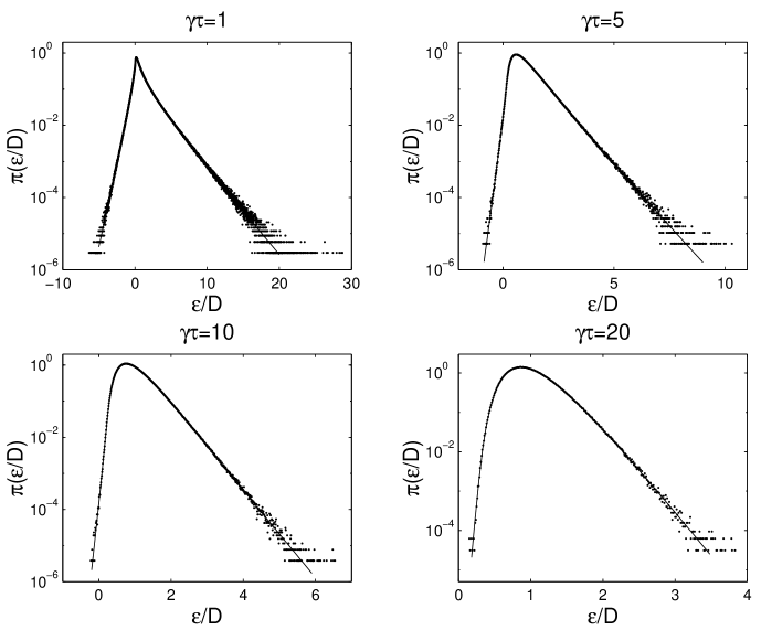
Figure 4: Semilog plots of the pdf of injected power $\pi(\tilde{\varepsilon})$ for several values of $\widetilde{\gamma}=\gamma\tau$. One plots together formula (39) (line) and results of numerical simulation (dots).

2.3 Discussion

These results address naturally some questions, in particular concerning the surprising structure of $f(\tilde{\varepsilon})$: this function displays a second order singularity located at a odd $\tilde{\varepsilon}=1/3$ value.

Let us first give some remarks on the shape of $\pi(\tilde{\varepsilon})$ (we restrict the discussion henceforth to situations where $\tau\gg\gamma^{-1}$). This pdf is a rather asymmetric curve, what can appear at first sight surprising : as the renewal of the noise $\psi$ is independent of the particle velocity $v$, occurrences of positive or negative instantaneous power injection $\psi v$ are completely equiprobable. Actually, the long time interval during which the mean is performed is of crucial importance and is responsible for the peculiar shape of the pdf; to understand this, let us consider an occurrence of a (rare) large positive fluctuation of injected power: this occurrence understands that a favourable sampling of the noise is realized, so that very often the noise gives energy to the particle. Consequently, during the process, the energy has a global tendency to increase, as well as typical values of the velocity (despite the always acting dissipation); as the injected power is directly proportional to the velocity, one sees that the direct effect of the positive injection of energy is to enhance typical values of $v$ implied in the evaluation of $\varepsilon$: this favourable feedback makes finally the occurrence of the considered fluctuation more likely, since less efficiency of the noise is globally required to generate the fluctuation.

On the contrary, let us consider a (large) negative fluctuation: the scenario is here inverted, since the typical velocity will certainly decrease during the mean process : to ensure the large expected value of power ceded back to the bath, one is then compelled to begin the motion with a large kinetic energy, what is exponentially unprobable : the feedback is here clearly unfavourable, and diminishes comparatively the frequency of such occurrences.

This primordial role of the initial energy on the negative power injection mechanism gives actually also the explanation for the presence of the negative tail in the large deviation function of $\pi(\tilde{\varepsilon})$: each fixed initial velocity is surely relaxed within a characteristic time $\propto\gamma^{-1}$, but this time is longer the higher initial velocity $v_{0}$; thus, when this velocity is statistically distributed according a Gaussian, rare large initial velocities construct the negative tail of the distribution as well as the associated large deviation function, which precisely characterizes rare events. It is worth to note that the specific negative tail due to the thermalization of $v_{0}$ begins actually at the value $1/3$, and thus affects substantially also the positive part of the distribution.

This singularity of the large deviation function can be interpreted as a phase transition, if one writes $\widehat{\pi}(\lambda)$ as a functional integral over the realizations of the noise $\psi$. Integration on $v_{0}$ gives

$$\widehat{\pi}(\lambda) \propto\int\mathcal{D}\psi\exp\left(-\frac{1}{4}\int_{0}^{\tau}\psi^{2}-\frac{\lambda D}{2}\int_{0}^{\tau}dt\ dt^{\prime}\ \psi(t)\psi(t^{\prime})e^{-\gamma|t-t^{\prime}|}+\frac{(\lambda D)^{2}}{2\gamma}\left[\int_{0}^{\tau}dt\ \psi(t)e^{-\gamma t}\right]^{2}\right)$$ (47)

and this expression can be viewed as a configurational partition function of an unidimensional line $\psi(t)$ of length $\tau$ confined in a quadratic potential $\mathcal{V}[\psi]\propto\int\psi^{2}$, with short range homogenous interactions (second term) and an additional local destabilization term (third term), which is a direct consequence of the thermalization of $v_{0}$. If $\lambda$ is positive and too large, the combined effects of the short range interaction term and the third term –which can be viewed more or less as an inverted parabolic potential acting in the vicinity of the $t=0$ end of the chain only– destabilizes the chain which is no longer confined by $\mathcal{V}$.

We would like to make here a little mathematical digression. One can compute the characteristic function from the preceding formula. This leads to the following formal expression

$$\widehat{\pi}(\lambda)=\exp\left(-\frac{1}{2}\sum_{n=1}^{\infty}\log\left(1+\frac{2\widetilde{\lambda}}{1+x_{n}^{2}}\right)\right.\\ \left.-\frac{1}{2}\log\left(1-4\widetilde{\lambda}^{2}\sum_{n=1}^{\infty}\frac{x_{n}^{2}}{1+x_{n}^{2}}\frac{1}{2+\widetilde{\gamma}(1+x_{n}^{2})}\frac{1}{1+2\widetilde{\lambda}+x_{n}^{2}}\right)\right)$$ (48)

where $x_{n}$ is solution of the implicit equation $\widetilde{\gamma}x_{n}+2\text{Atan}x_{n}=n\pi$. That this involved expression is exactly the simple formula (18) is quite amazing, and one can derive some nontrivial mathematical relations from this connection; to mention but a few, one has for instance

$$\sum_{n=1}^{\infty}\frac{1}{1+x_{n}^{2}}=\frac{\widetilde{\gamma}}{2}$$ (49)

a relation which is easily checked for $\widetilde{\gamma}\rightarrow 0$ ($x_{1}\sim\sqrt{2/\widetilde{\gamma}}$) and $\widetilde{\gamma}\rightarrow\infty$ (the sum becomes a Riemanian sum).

To conclude this paragraph, it is important to note that, in contradiction with intuition, initial conditions can have deep consequences on the shape of large deviations functions, even if the process displays finite time correlations, provided that these initial conditions are statistically distributed over an unbounded interval, what is almost always the case if for instance stationary processes are considered.

2.4 Dissipated Power

The pdf of dissipated power can also be computed along the same line of reasoning. One gets for the characteristic function of the stationary process:

$$\left\langle\exp-\lambda\gamma\int_{0}^{\tau}dt\ v^{2}(t)\right\rangle =e^{\widetilde{\gamma}/2}\left(\cosh\eta\widetilde{\gamma}+\eta\sinh\eta\widetilde{\gamma}\right)^{-\frac{1}{2}}$$ (50)

and one sees that there is not any positive cut in that case. As a result, the large deviation function of the stationary dissipated power $\delta=\frac{1}{\tau}\int_{0}^{\tau}\gamma v^{2}$ is easily derived as $f_{dissip}(\delta)=f_{0}(\delta)$. Consequently, one expects the pdf of dimensionless injected and dissipated power to be (in the large $\tau$ limit) similar but in the zero injection (or dissipation) region. This is effectively the case, as shown on figure 5.

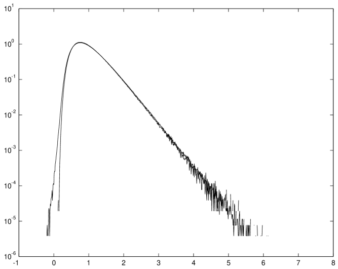
Figure 5: Injected and dissipated power pdf for the free Brownian motion ($\gamma\tau=10,D=1$). The two distributions are very similar but in the vicinity of zero, partly due to the constraint $\gamma v^{2}\geqslant 0$, whereas $\psi v\gtrless 0$.

2.5 Note on the Fluctuation Theorem

As explained in the introduction, our model is a good system to test the possible universality of the conclusions of the (Evans-Cohen-Morris) fluctuation theorem, since the exact result is at hand. From (46), one has

$$\rho(\tilde{\varepsilon})\equiv\frac{1}{\tau}\log\frac{\pi(\tilde{\varepsilon})}{\pi(-\tilde{\varepsilon})} {\displaystyle\mathop{\sim}_{\tau\rightarrow\infty}}\left\{\begin{array}[]{ll}\displaystyle 4\gamma\tilde{\varepsilon}&\mbox{if $\tilde{\varepsilon}<1/3$}\\ \displaystyle\frac{7}{4}\gamma\tilde{\varepsilon}+\frac{3}{2}\gamma-\frac{\gamma}{4\tilde{\varepsilon}}&\mbox{if $\tilde{\varepsilon}>1/3$}\end{array}\right.$$ (53)

This function is clearly not a straight line, as it would be if the FT held here (not even the slope at $\tilde{\varepsilon}=0$ is in accordance with the FT, which would predict $\rho(\tilde{\varepsilon})=\gamma\tilde{\varepsilon}$). Thus we exhibit here an example where the conclusions of the theorem are not verified (due to the simple fact that the situation considered here does not fulfill the hypotheses required for the Fluctuation Theorem to hold). On this “negative” result can we make two comments: first, it is not contradictory with those of Kurchan [9]. One looks for the power injected by a random fluctuation in a dissipative system, whereas the Fluctuation Theorem established by Kurchan considers the power injected by an external operator in a system in equilibrium with a thermostat. We already noticed that the first situation is much more appropriate to describe realistic systems driven far from equilibrium. Second, formula (53) illustrates well the fact that Fluctuation Theorem seems to hold in so large a number of experimental situations, as explained in [4]: in the vicinity of $\tilde{\varepsilon}=0$, $\rho(\tilde{\varepsilon})$ must always have a straight line behaviour, as a consequence of the large deviation law; on the other hand, as large negative values of $\tilde{\varepsilon}$ are extremely unprobable when $\tau$ is large, it becomes practically unpossible even to only measure $\rho(\tilde{\varepsilon})$ for large $\tilde{\varepsilon}$ and large $\tau$ with enough statistical resolution: possible deviations from the straight line are just even not measurable. In our case, crossover occurs for $\tilde{\varepsilon}=1/3$ and for this value, $\pi\propto\exp(-5\gamma\tau/3)$ which is of order $10^{-8}$ only if $\gamma\tau=10$…Our model is thus a good illustration in favour of arguments given in [4] against an universal applicability of conclusions of the Fluctuation Theorem.

Figure 6: Function $\tau^{-1}\log[{\pi}(\tilde{\varepsilon})/\pi(-\tilde{\varepsilon})]$ for $\gamma\tau=8$. Circles come from numerics with two millions points of statistics, and stop before the crossover of the theoretical curve (solid) due to the lack of negative points with large absolute value.

3 Confined Brownian Motion

The reasoning concerning the asymmetry of $\pi(\tilde{\varepsilon})$ suggests that certain characteristics of this pdf seem —in the limit of large $\tau$ only— to be independent of the details of the particle dynamics, since it is based only on considerations on energy and its conservative character. These observations led us to infer a possible insensivity of $\pi$ with respect to other microscopic times than $\gamma^{-1}$ ($\gamma^{-1}$ itself cannot be neglected, since this time plays a role in the process of dissipation of energy; and indeed, the curves for different $\gamma$ have different and non superposable shapes), in cases where the initial system would have been complexified. Thus, we considered several confined Langevin systems:

$$\ddot{x}+\gamma\dot{x}+V^{\prime}(x) =\psi(t)$$ (54)

$$<\psi(t)\psi(t^{\prime})> =2D\delta(t-t^{\prime})$$ (55)

where we used for $V(x)$ an harmonic potential $V(x)=\frac{1}{2}\omega^{2}x^{2}$, a non linear “hard” potential $V(x)=\frac{1}{2}\omega^{2}x^{2}+\frac{\alpha}{4}x^{4}$ ($\alpha>0$), a non linear asymmetric “soft” potential $V(x)=\omega^{2}(\alpha^{2}e^{-x/\alpha}+\alpha x)$, and also a bistable $\varphi^{4}$ potential $V(x)=V_{b}(x^{2}-1)^{2}$. We numerically calculated for all these potentials (as well as again the free case for comparison) the pdf $\pi(\tilde{\varepsilon})$, for large values of $\tau$ ($\gamma=1$ for convenience).

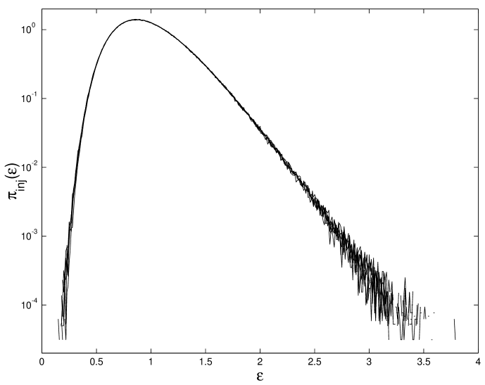
Figure 7: Injected power pdf for several trapped Langevin particles with $D=1$, $\tau=20$ and $\gamma=1$ : three harmonic potentials (free motion $\omega=0$, $\omega=1$ and $\omega=10$), hard and soft nonlinear potentials ($\omega=1$,$\alpha=3$ in both cases), bistable $\varphi^{4}$-potential with $V_{b}=1$ (strong anharmonicity is explored in this case – see details in text).

The results (see fig. 7) are extraordinarily surprising, since one cannot distinguish the different curves from each other! One must keep in mind the fact that the dynamical behaviour of $x(t)$ is completely different in all these cases: fully isochronic or anisochronic oscillatory, overdamped, bistable, diffusive, these different Brownian motions lead all to apparently the same curve, a coincidence which goes beyond all expectations.

To understand this phenomenon, let us look at the characteristic function $\widehat{\pi}_{\mathbf{r_{0}}}(\lambda)$, where $\mathbf{r_{0}}=(x_{0},v_{0})$ designates the initial conditions. Of course, one cannot compute it exactly, since in general the dynamics is nonlinear. Nevertheless, it is possible to express it in a fruitful form.

From [13], one can derive the path integral representation of the solution of the Kramers equation:

$$P_{\gamma}(\mathbf{r_{1}},\tau|\mathbf{r_{0}},0) =e^{\widetilde{\gamma}/2}\times\int_{\mathbf{r}(0)=\mathbf{r_{0}}}^{\mathbf{r}(\tau)=\mathbf{r_{1}}}[\mathcal{D}x]\exp\left(-\frac{1}{4D}\int_{0}^{\tau}dt\ [\ddot{x}+\gamma\dot{x}+V^{\prime}(x)]^{2}\right)$$ (56)

(the index $\gamma$ recalls the value of the damping). As before, one gets from this

$$\widehat{\pi}_{\mathbf{r_{0}}}(\lambda)=\int d\mathbf{r_{1}}\int_{\mathbf{r}(0)=\mathbf{r_{0}}}^{\mathbf{r}(\tau)=\mathbf{r_{1}}}[\mathcal{D}x]\exp\left(\frac{\widetilde{\gamma}}{2}-\frac{1}{4D}\int_{0}^{\tau}dt\ [\ddot{x}+\gamma\dot{x}+V^{\prime}(x)]^{2}-\lambda\int_{0}^{\tau}\dot{x}[\ddot{x}+\gamma\dot{x}+V^{\prime}(x)]\right)$$ (57)

After some simple manipulations, one can recast this into

$$\widehat{\pi}_{\mathbf{r_{0}}}(\lambda)=e^{\frac{\widetilde{\gamma}}{2}(1-\eta)}\int d\mathbf{r_{1}}P_{\gamma\eta}(\mathbf{r_{1}},\tau|\mathbf{r_{0}},0)\times\exp\left(-\frac{\gamma}{2D}(\widetilde{\lambda}+1-\sqrt{1+2\widetilde{\lambda}})(E_{1}-E_{0})\right)$$ (58)

where $E_{i}=\frac{1}{2}\dot{x}_{i}^{2}+V(x_{i})$ (we recall $\widetilde{\lambda}=2D\lambda/\gamma,\eta=\sqrt{1+2\widetilde{\lambda}}$). This formula is useful, since the propagator $P_{\eta\gamma}$ goes exponentially fast to the equilibrium value $P_{eq}(\mathbf{r_{1}})=\sqrt{\gamma\eta/(2\pi D)}U_{\eta}^{-1}\exp(-\gamma\eta E_{1}/D)$ where $U_{\alpha}\equiv\int dx_{0}\exp(-\gamma\alpha V(x_{0})/D)$ is the configurational partition function. Consequently, for each fixed value of $\mathbf{r_{0}}$, one has the true equivalence

$$\widehat{\pi}_{\mathbf{r_{0}}}(\lambda) \sim\sqrt{\frac{\gamma\eta}{2\pi D}}U_{\eta}^{-1}e^{\frac{\widetilde{\gamma}}{2}(1-\eta)}\int d\mathbf{r_{1}}\exp\left(-\frac{\gamma}{2D}[(\widetilde{\lambda}+1+\eta)E_{1}-(\widetilde{\lambda}+1-\eta)E_{0}]\right)$$ (59)

and one sees that there is no problem of convergence in the integral for any real value of $\widetilde{\lambda}$ such that $\widetilde{\lambda}>-1/2$ (for $\widetilde{\lambda}<-1/2$ there is always a cut due to the presence of a square root in $\eta$). Thus, one extracts exactly the leading exponential term from the preceding formula as

$$\log\widehat{\pi}_{\mathbf{r_{0}}}(\lambda) \sim\frac{\widetilde{\gamma}}{2}(1-\eta)$$ (60)

and shows in the same time that the large deviation function of $\pi_{\mathbf{r_{0}}}(\tilde{\varepsilon})$ is

$$f_{\mathbf{r_{0}}}(\tilde{\varepsilon})=-\frac{\gamma}{4\tilde{\varepsilon}}(\tilde{\varepsilon}-1)^{2}\times\theta(\tilde{\varepsilon})$$ (61)

irrespective of the precise form of the potential.

Let us now look at $\pi(\tilde{\varepsilon})$: its characteristic function can be written

$$\widehat{\pi}(\lambda)=\sqrt{\frac{\gamma}{2\pi D}}\frac{e^{\frac{\widetilde{\gamma}}{2}(1-\eta)}}{U_{1}}\int d\mathbf{r_{0}}d\mathbf{r_{1}}P_{\gamma\eta}(\mathbf{r_{1}},\tau|\mathbf{r_{0}},0)\times\exp\left(-\frac{\gamma}{2D}[(\widetilde{\lambda}+1-\eta)E_{1}-(\widetilde{\lambda}-1-\eta)E_{0}]\right)$$ (62)

A priori, one must take care of the fact that the equivalence $P(\mathbf{r_{1}},\tau|\mathbf{r_{0}},0)\sim P_{eq}(\mathbf{r_{1}})$ is not reached uniformly with respect to $\mathbf{r_{0}}$, as already noticed. But, if one inspects the free Brownian case, for which the exact result is computed, this replacement is finally equivalent to neglect exponentially small corrections (terms like $\tanh\eta\widetilde{\gamma}$ replaced by $1$ for instance); this is precisely this approximation which leads to formulæ (42,43) from (40,41): the only limitation is that the resulting formulæ  are not uniformly valid in the $\tilde{\varepsilon}$ space. But the associated large deviation function is unaffected by these corrections.

We can assume that this scenario is still correct in the general case, an assumption which is very reasonable indeed. Thus, up to exponentially vanishing factors, one has

$$\widehat{\pi}(\lambda) \sim\frac{\gamma\sqrt{\eta}}{2\pi D}\times\frac{e^{\frac{\widetilde{\gamma}}{2}(1-\eta)}}{U_{1}U_{\eta}}\int d\mathbf{r_{0}}d\mathbf{r_{1}}\exp\left(-\frac{\gamma}{2D}[(\widetilde{\lambda}+1+\eta)E_{1}-(\widetilde{\lambda}-1-\eta)E_{0}]\right)$$ (63)

$$=\sqrt{\frac{4\eta}{(\eta+1)^{2}-\widetilde{\lambda}^{2}}}\times e^{\frac{\widetilde{\gamma}}{2}(1-\eta)}\times\frac{U_{(\widetilde{\lambda}+1+\eta)/2}U_{(\eta+1-\widetilde{\lambda})/2}}{U_{1}U_{\eta}}$$ (64)

and it is easily seen that, again, the $\mathbf{r_{0}}$ integral diverges when $\widetilde{\lambda}$ approaches $\widetilde{\lambda}_{+}=4$, pointing out the probable beginning of a real cut, already encountered when $V=0$. Noticing that the leading exponential term is $\exp(\frac{\widetilde{\gamma}}{2}(1-\eta))$, also insensitive to the presence of a pinning potential, one deduces that also in this case the large deviation function is given by (46). Of course, fully mathematical precision is not given here, but we think that convincing arguments are nevertheless given in favour of our result.

Concerning the prefactor of the large deviation function, it is interesting to mention that it keeps in general a dependence on the form of the pinning potential, through the functions $U$. In fact, formulas like (42,43) can themselves be simplified; for instance

$$J(\tilde{\varepsilon})\sim\left(\frac{4\widetilde{\gamma}}{\pi(3\tilde{\varepsilon}-1)(\tilde{\varepsilon}+1)^{3}}\right)^{\frac{1}{2}}$$ (65)

(we did not propose this equivalence previously, for it is not correct in the vicinity of $\tilde{\varepsilon}=1/3$, unlike formula (42)…). For the general case with a potential $V$, this “supersimplification” gives

$$J(\tilde{\varepsilon})\sim\left(\frac{4\widetilde{\gamma}}{\pi(3\tilde{\varepsilon}-1)(\tilde{\varepsilon}+1)^{3}}\right)^{\frac{1}{2}}\times\frac{U_{(\tilde{\varepsilon}^{-1}+1)^{2}/4}U_{(3-\tilde{\varepsilon}^{-1})(1+\tilde{\varepsilon}^{-1})/4}}{U_{1}U_{\tilde{\varepsilon}^{-1}}}$$ (66)

Thus, the pdf associated with different potentials do not exactly coincide at large $\tau$, except at the value $\tilde{\varepsilon}=1$. But, at the level of the large deviation function, the universality of $f(\tilde{\varepsilon})$ is reached. The combination of these two points explains probably the remarkable coincidence of the different curves on the figure 7.

4 Conclusion

In this paper, we considered the Langevin equation as a dynamical evolution of a simple dissipative system driven by an external forcing, and computed the probability density function of the time-averaged injected power in the permanent and non permanent regimes. We showed that the associated large deviation functions are different, in particular a negative tail exists only in the permanent regime. We explained the origins of this discrepancy and highlighted the role of the rare but very energetic initial conditions; we showed also that the system considered here does not verify the so-called Fluctuation Relation $f(\tilde{\varepsilon})-f(-\tilde{\varepsilon})=\gamma\tilde{\varepsilon}$, even in the vicinity of $\tilde{\varepsilon}=0$, indicating thence that any attempt to enlarge careless the applicability of the conclusions of the Fluctuation Theorem to dissipative systems is vain.

We considered thereafter Langevin equations with pinning potential, and showed that the associated large deviation functions are completely insensitive to the potential (but not the pdf itself): this result appears to be a good indication that large deviation functions could be an appropriate tool to characterize well general properties of systems beyond some peculiar irrelevant details which faded away through the process of averaging. In our case, the function $f$ tells us something global associated with the energy transfer throughout the Brownian particle, irrespective to the precise dynamics of each geometrical configuration.

A natural extension will be to consider stochastic coloured dynamics, i.e. noises with time correlation. We want to test the “solidity” of $f$ with respect to correlations arising in the external forcing. Moreover, we can address the question of the generality of the observed non-analyticity of the large deviation function in systems in permanent regime where the velocity field is unbounded: from our analysis of the Langevin system, we think that such anomalies could be widely encountered in dissipative far-from-equilibrium systems. An interesting perspective is besides to consider extremely correlated noises, in order to check in this context the ideas exposed in [15, 16], where some conjectures are made on the limiting behaviours of the pdf of global variables in highly correlated systems.

5 Acknowledgments

I am much indebted to S.Fauve, R.Labbé, S.Aumaître, F.Pétrelis, R.Berthet, N.Mujica, R.Wunenburger and B.Derrida for fruitful discussions. I acknowledge also a referee for having suggested me an alternative and fruitful technical approach of the computation.

References

• [1] R.Labbรฉ, J.F.Pinton, S.Fauve, J.Phys. II France, 6 (1996) 1099.
• [2] S.Aumaรฎtre, S.Fauve, J. Chim. Phys., 96 (1999), 1038.
• [3] S.Aumaรฎtre, S.Fauve, J.F.Pinton, Eur. Phys. J. B., 16 (2000), 563.
• [4] S.Aumaรฎtre, S.Fauve, S.McNamara, P.Poggi, Eur. Phys. J. B, 19 (2001), 449.
• [5] S.Ciliberto, C.Laroche, J. Phys. IV (France), 8, Pr6-215 (1998).
• [6] S.I. Sasa, cond-mat/0010026.
• [7] D.J.Evans, E.G.D. Cohen, G.P.Morris, Phys. Rev. Lett., 71 (1993), 2041.
• [8] G.Gallavotti, E.G.D. Cohen, Phys. Rev. Lett., 74 (1995), 2694.
• [9] J.Kurchan, J.Phys. A,31 (1998), 3719.
• [10] B. Derrida & C. Appert, J. Stat. Phys., 94, 1 (1999). B.Derrida & J.L.Lebowitz, Phys. Rev. Lett., 80, 209 (1998).
• [11] F.W. Wiegel, Introduction to Path-Integral Methods in Physics and Polymer Science, World Scientific.
• [12] R.P. Feynman, Statistical Mechanics, Frontiers in Physics, Benjamin/Cummings.
• [13] J. Zinn-Justin, Quantum Field Theory and Critical Phenomena, Oxford University Press.
• [14] C.M. Bender & S.A. Orszag, Advanced Mathematical Methods for Scientists and Engineers, Springer.
• [15] S.T. Bramwell, P.C.W. Holdsworth, J.F. Pinton, Nature, 396, 552 (1998).
• [16] S.T. Bramwell, K. Christiensen, J.Y. Fortin, P.C.W. Holdsworth, H.J. Jensen, S. Lise, J. Lรณpez, M. Nicodemi, J.F. Pinton, M. Sellitto, Phys. Rev. Lett., 84, 3744 (2000).