Heavy Quasi-Particles in the Two-Orbital Hubbard Model

1 Introduction

Strongly correlated electron systems, such as the high-$T_{\rm c}$ superconductors ${}^{\hbox{\immediate{\bf{?}})}}$ and the heavy fermion compounds ,${}^{\hbox{\immediate{\bf{?}})}}$ have attracted much interest. In order to deal with electron correlations, the single-orbital Hubbard model ${}^{\hbox{\immediate{\bf{?}},\penalty 1000\hskip 0.91003pt plus 0.70004pt minus 0.70004pt{\bf{?}},\penalty 1000\hskip 0.91003pt plus 0.70004pt minus 0.70004pt{\bf{?}})}}$ has been studied extensively with various analytical and numerical methods. Among others, dynamical mean field theory (DMFT) ${}^{\hbox{\immediate{\bf{?}})}}$ enables us to systematically investigate strong correlation effects. By using DMFT characteristic properties related to the Mott transition has been described successfully for the single orbital case.${}^{\hbox{\immediate{?})}}$

In real materials such as the transition metal oxides,${}^{\hbox{\immediate{?})}}$ orbital degeneracy plays an important role, giving rise to a wide variety of interesting phenomena. In such cases the Hund coupling and the orbital splitting are the additional key parameters to discuss electron correlations. It is thus desirable to study the orbitally degenerate Hubbard model in order to better understand strongly correlated electron systems. Recently, a number of theoretical studies on the orbitally degenerate Hubbard model have been done by using the slave-boson mean field approximation ,${}^{\hbox{\immediate{\bf{?}},\penalty 1000\hskip 0.91003pt plus 0.70004pt minus 0.70004pt{\bf{?}},\penalty 1000\hskip 0.91003pt plus 0.70004pt minus 0.70004pt{\bf{?}})}}$ the quantum Monte Carlo method ${}^{\hbox{\immediate{\bf{?}})}}$ and DMFT .${}^{\hbox{\immediate{\bf{?}},\penalty 1000\hskip 0.91003pt plus 0.70004pt minus 0.70004pt{\bf{?}},\penalty 1000\hskip 0.91003pt plus 0.70004pt minus 0.70004pt{\bf{?}},\penalty 1000\hskip 0.91003pt plus 0.70004pt minus 0.70004pt{\bf{?}},\penalty 1000\hskip 0.91003pt plus 0.70004pt minus 0.70004pt{\bf{?}})}}$

In this paper, we systematically study electron correlations for the two-orbital Hubbard model with particular emphasis on the interplay of the Hubbard interaction, the Hund coupling and the orbital splitting. By employing DMFT combined with the non-crossing approximation (NCA), we compute the one-particle spectral function and the optical conductivity. We discuss how the heavy quasi-particle behavior shows up in a metallic state close to the Mott insulator with orbital degeneracy. We find that the origin of heavy quasi-particles can be different between quarter filling and half filling. In particular, we point out that the Hund coupling plays an essential role to form a heavy quasi-particle band in the vicinity of half filling.

This paper is organized as follows. In the next section, we briefly describe the model and the method, and then in §3 we show the results obtained for the one-particle spectral function and the optical conductivity. A brief summary is given in §4.

2 Model and Method

2.1 Two-Orbital Hubbard Hamiltonian

We study the Hubbard model with two orbitals. The Hamiltonian is given by

$$H = \sum_{<i,j>}\sum_{m,m^{\prime},\sigma}t^{mm^{\prime}}_{ij}c^{{\dagger}}_{im\sigma}c_{jm^{\prime}\sigma}+\frac{\Delta}{2}\sum_{i,\sigma}(n_{i1\sigma}-n_{i2\sigma})$$ (2.1)

$$+ U^{\prime}\sum_{i,m}n_{im\uparrow}n_{im\downarrow}+U\sum_{i,\sigma}n_{i1\sigma}n_{i2\bar{\sigma}}$$

$$+ (U-J)\sum_{i,\sigma}n_{i1\sigma}n_{i2\sigma}$$

$$- J\sum_{i}(c^{{\dagger}}_{i1\uparrow}c_{i1\downarrow}c^{{\dagger}}_{i2\downarrow}c_{i2\uparrow}+h.c.),$$

where $c_{im\sigma}(c^{{\dagger}}_{im\sigma})$ is the annihilation (creation) operator of electrons with the orbital $m(=1,2)$ and spin $\sigma(=\uparrow,\downarrow)$ at the site $i$ and $\Delta$ represents the energy splitting between the two orbitals. Here, $U^{\prime}(U)$ is the Coulomb repulsion between electrons in the same (different) orbital and $J$ is the ferromagnetic Hund coupling. When the two orbital-levels are degenerate ($\Delta=0$), the system is rotationally invariant with respect to the spin and orbital degrees of freedom, leading to the condition, $U^{\prime}=U+J$. We use this relation and assume that the hopping is diagonal with respect to the orbital indices ($t^{mm^{\prime}}_{ij}=-t\delta_{mm^{\prime}}$). We shall deal with a paramagnetic metallic phase close to the Mott insulator in this paper.

2.2 Dynamical Mean Field Theory

It is known that DMFT is justified in the limit of large spatial dimensions ${}^{\hbox{\immediate{\bf{?}},\penalty 1000\hskip 0.91003pt plus 0.70004pt minus 0.70004pt{\bf{?}})}}$ and gives a rather good approximation even in three dimensions. In this method, a lattice electron problem is replaced by the corresponding impurity one embedded in an effective medium determined self-consistently. The effective local Hamiltonian is given by

$$H_{\rm eff} = H_{\rm loc}+H_{\rm med},$$ (2.2)

$$H_{\rm loc} = \sum_{m,\sigma}E_{fm}n_{m\sigma}+U^{\prime}\sum_{m}n_{m\uparrow}n_{m\downarrow}$$ (2.3)

$$+ U\sum_{\sigma}n_{1\sigma}n_{2\bar{\sigma}}+(U-J)\sum_{\sigma}n_{1\sigma}n_{2\sigma}$$

$$- J(c^{{\dagger}}_{1\uparrow}c_{1\downarrow}c^{{\dagger}}_{2\downarrow}c_{2\uparrow}+h.c.),$$

$$H_{\rm med} = \sum_{km\sigma}(V_{km\sigma}a^{{\dagger}}_{km\sigma}c_{m\sigma}+h.c.)$$ (2.4)

$$+ \sum_{km\sigma}\epsilon_{k}a^{{\dagger}}_{km\sigma}a_{km\sigma},$$

where the impurity level in the reduced problem is

$$E_{{f}m}=\left\{\begin{array}[]{cc}E_{f}+\Delta/2&({\rm orbital\,1})\\ E_{f}-\Delta/2&({\rm orbital\,2})\end{array}\right.$$ (2.7)

Here, $V_{km\sigma}$ represents the hybridization between the impurity site and an effective medium.

Let us first introduce the so-called cavity Green function and the full Green function, which are defined respectively as

$${\cal G}_{0m\sigma}(\omega) = [\omega+{\rm i}\delta+\mu-E_{fm}-\Delta_{m\sigma}(\omega)]^{-1}$$ (2.8)

$$G_{m\sigma}(\omega) = [{\cal G}_{0m\sigma}^{-1}(\omega)-\Sigma_{m\sigma}(\omega)]^{-1}$$ (2.9)

where $\mu$ is the chemical potential. Here $\Delta_{m\sigma}(\omega)$ represents the hybridization function given by

$$\Delta_{m\sigma}(\omega)=\frac{1}{N}\sum_{k}\frac{|V_{km\sigma}|^{2}}{\omega+{\rm i}\delta-\epsilon_{k}}.$$ (2.10)

In DMFT, the self-consistency equation is given by

$$G_{m\sigma}(\omega)=$$

$$[\omega+{\rm i}\delta+\mu-E_{fm}-\Sigma_{m\sigma}(\omega)-\frac{D^{2}}{4}G_{m\sigma}(\omega)]^{-1},$$ (2.11)

where we have employed the semi-elliptic density of states for non-interacting electrons, $N_{0}(\epsilon)=2/(\pi D^{2})\sqrt{D^{2}-\epsilon^{2}}$ with the bandwidth $D$.

In order to solve the effective impurity problem, we further use NCA,${}^{\hbox{\immediate{\bf{?}},\penalty 1000\hskip 0.91003pt plus 0.70004pt minus 0.70004pt{\bf{?}},\penalty 1000\hskip 0.91003pt plus 0.70004pt minus 0.70004pt{\bf{?}},\penalty 1000\hskip 0.91003pt plus 0.70004pt minus 0.70004pt{\bf{?}},\penalty 1000\hskip 0.91003pt plus 0.70004pt minus 0.70004pt{\bf{?}},\penalty 1000\hskip 0.91003pt plus 0.70004pt minus 0.70004pt{\bf{?}},\penalty 1000\hskip 0.91003pt plus 0.70004pt minus 0.70004pt{\bf{?}})}}$ which is known to provide rather reliable results in agreement with the quantum Monte Carlo calculation ${}^{\hbox{\immediate{?})}}$ for the single-orbital case. We first diagonalize the local Hamiltonian $H_{\rm loc}$,

$$H_{\rm loc}=\sum^{16}_{\alpha=1}E_{\alpha}|\alpha\rangle\langle\alpha|,$$ (2.12)

where $|\alpha\rangle$ and $E_{\alpha}$ denote the spin-orbital eigenstate and the corresponding energy for the isolated ionic system. Using these eigenstates, the fermionic annihilation operator is represented as

$$c_{m\sigma} = \sum_{\alpha,\alpha^{\prime}}D^{m\sigma}_{\alpha\alpha^{\prime}}|\alpha\rangle\langle\alpha^{\prime}|,$$ (2.13)

$$D^{m\sigma}_{\alpha\alpha^{\prime}} = \langle\alpha|c_{m\sigma}|\alpha^{\prime}\rangle.$$ (2.14)

We now introduce the ionic resolvent and its self-energy, which are represented in terms of the basis set $|\alpha\rangle$ as,

$$R_{\alpha}(\omega) =[\omega-E_{\alpha}-\Sigma_{\alpha}(\omega)]^{-1},$$

$$\Sigma_{\alpha}(\omega) =\sum_{m\sigma}\sum_{\alpha^{\prime}}(|D^{m\sigma}_{\alpha\alpha^{\prime}}|^{2}+|D^{m\sigma}_{\alpha^{\prime}\alpha}|^{2})$$

$$\times\int^{\infty}_{\infty} {\rm d}\epsilon\,f(\eta_{\alpha\alpha^{\prime}}\epsilon)\Delta_{m\sigma}(\epsilon)R_{\alpha^{\prime}}(\omega+\eta_{\alpha\alpha^{\prime}}\epsilon),$$ (2.16)

with the Fermi distribution function $f(\epsilon)$, where $\eta_{\alpha\alpha^{\prime}}$ takes $1(-1)$ if the particle number of the state $|\alpha\rangle$ is larger (smaller) than that of $|\alpha^{\prime}\rangle$. In eq.(2.16), we have neglected the vertex corrections, as often done in the treatment of DMFT. The full Green function is now given by

$$G_{m\sigma}(\omega)=\sum_{\alpha\alpha^{\prime}}|D^{m\sigma}_{\alpha\alpha^{\prime}}|^{2}{\tilde{G}}_{\alpha\alpha^{\prime}}(\omega),$$ (2.17)

where ${\tilde{G}}_{\alpha\alpha^{\prime}}(\omega)$ is written in terms of the ionic resolvents,

$${\tilde{G}}_{\alpha\alpha^{\prime}}(\omega)=\frac{1}{Z}\int{\rm d}\epsilon\,{\rm e}^{-\beta\epsilon}$$ (2.18)

$$\times [\rho_{\alpha}(\epsilon)R_{\alpha^{\prime}}(\omega+\epsilon)-\rho_{\alpha^{\prime}}(\epsilon)R_{\alpha}(\epsilon-\omega)]$$

and

$$Z=\sum_{\alpha}\int{\rm d}\epsilon\,{\rm e}^{-\beta\epsilon}\rho_{\alpha}(\epsilon).$$ (2.19)

In eq. (2.18) and (2.19), $\rho_{\alpha}(\omega)=-1/\pi{\rm Im}(R_{\alpha}(\omega))$ is the spectral function of the ionic resolvent.

This completes the self-consistent procedure for DMFT with NCA.

3 Numerical Results

We numerically iterate the procedure in the previous section until the calculated quantities converge within desired accuracy. In the following discussions, the bandwidth $D$ is taken to be unity for simplicity.

3.1 Heavy quasi-particles near quarter filling

Let us start with a metallic system close to quarter filling ($n_{\rm tot}\sim 1$). We calculate the one-particle spectral function defined by

$$\rho_{m\sigma}(\omega)=-\frac{1}{\pi}{\rm Im}\,G_{m\sigma}(\omega)$$ (3.1)

for several different values of the Hubbard interaction $U$. We first discuss the case in the absence of the Hund coupling, $J=0$. The results are shown in Fig.1.

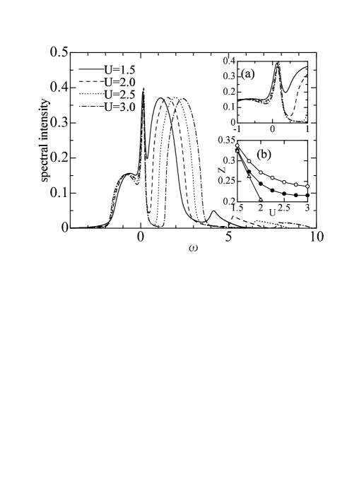
Fig.  1: One-particle spectral function $\rho_{m\sigma}(\omega)$ at $T=0.1$ for $J=0$ and $\Delta=0$. The electron density per site is $n_{\rm tot}=0.96$ (i.e. close to quarter filling). The energy is measured from the Fermi level $\omega=0$, and the bandwidth $D$ is taken to be unity. The inset (a) shows the magnification of the low-frequency part, while (b) shows the quasi-particle renormalization factor $Z$ as a function of $U$ for $n_{\rm tot}=0.96$ (open circles), $n_{\rm tot}=0.98$ (filled circles) and $n_{\rm tot}=1.00$ (triangles).

As the Hubbard interaction increases, a sharp peak structure appears and gets narrower around the Fermi level, which is caused by the formation of heavy quasi-particles.${}^{\hbox{\immediate{?},\penalty 1000\hskip 0.91003pt plus 0.70004pt minus 0.70004pt{?},\penalty 1000\hskip 0.91003pt plus 0.70004pt minus 0.70004pt{\bf{?}})}}$ At the same time, it is seen that a pseudo-gap structure develops just above the Fermi level because the Hubbard interaction suppresses the charge fluctuation while enhances the spin fluctuation near quarter filling. This behavior is similar to that expected for the hole-doped Hubbard model with single orbital. The other peaks are easily identified with the singly, doubly and triply occupied states, respectively. The intensity of the fully occupied state is too small to observe in this figure.

The formation of a heavy quasi-particle band is more clearly seen in the quasi-particle renormalization factor shown in the inset (b) of Fig.1, which is defined by

$$Z={\biggl{[}}1-\frac{\partial\Sigma(\omega)}{\partial\omega}{{\hbox{$\left|\vbox to0.0pt{}\right.\n@space$}}}_{\omega=0}{\biggr{]}}^{-1}.$$ (3.2)

Since the mass enhancement factor of quasi-particles is inversely proportional to the renormalization factor, it is confirmed that the mass of the renormalized band indeed increases as the Hubbard interaction $U$ increases.

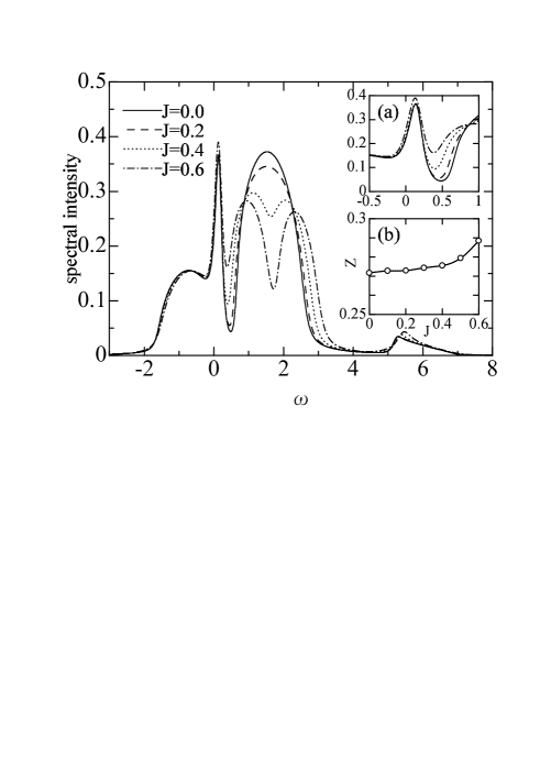
Fig.  2: One particle spectral function for various $J$ at $T=0.1$ and $U=2$. The electron concentration is $0.96$. The insets (a) and (b) show the magnification of the low-frequency behavior and the renormalization factor.

In Fig. 2, we show how the Hund coupling $J$ affects the spectral properties near quarter filling. Although the spectral weight for the doubly occupied state splits into two parts as $J$ increases, the quasi-particle spectrum near the Fermi level is not so much affected by weak or intermediate $J$. In particular, for the strong Hubbard interaction, the Hund coupling hardly affects the quasi-particle mass although it modifies the spectrum in the high energy regime.

Similarly, even when the splitting between two orbitals is introduced, the formation of quasi-particles is not so much affected, as seen from Fig. 3.

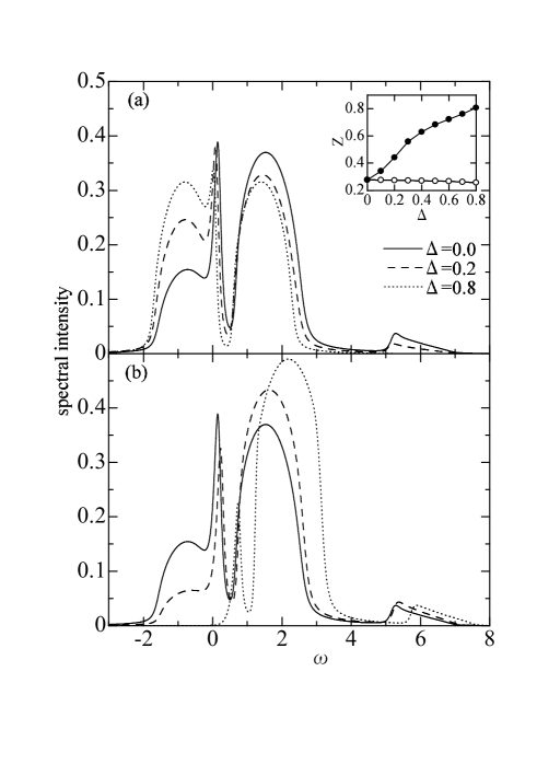
Fig.  3: One particle spectral function for $U=2$, $J=0$ and $T=0.1$: (a) lower band and (b) upper band. The electron concentration is $n_{\rm tot}=0.96$. The inset shows the renormalization factor for lower band (open circles) and upper band (filled circles).

For the lower band, the spectral weight is gradually transferred from the doubly and triply occupied states to the singly occupied state as $\Delta$ increases, while for the upper band, the weight for the singly occupied state decreases, as should be expected. Note that a quasi-particle band always exists in the lower band irrespective of $\Delta$. We can check that the renormalization factor for the lower band is almost unchanged as a function of $\Delta$. (Fig. 3, inset) For sufficiently large $\Delta$, the spectrum of the lower band is reduced to that of the single-orbital model near half filling, which is indeed seen in the case of $\Delta=0.8$.

Summarizing, the formation of heavy quasi-particles near quarter filling is caused by the Hubbard interaction, as is the case for the single-orbital model. In particular, a heavy quasi-particle band and a pseudo-gap structure are almost always formed for reasonably large $U$, irrespective of the strength of the orbital splitting and the Hund coupling. As we will see momentarily, this is not the case for the formation of heavy quasi-particles near half filling.

3.2 Heavy quasi-particles near half filling

We now turn to a metallic system close to half-filling ($n_{\rm tot}\sim 2$). Let us first discuss the system without orbital splitting. Fig.4 shows the one-particle spectrum as a function of the Hund coupling $J$.

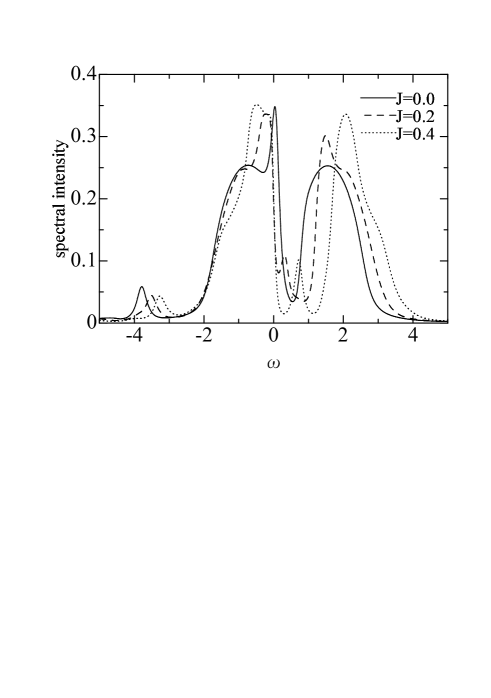
Fig.  4: One particle spectral function near half filling, $n_{\rm tot}=1.90$: $U=2$, $\Delta=0$ and $T=0.1$.

As mentioned above, a heavy quasi-particle band exists around the Fermi level for $U=2$. In contrast to the quarter filling case, the spectrum near the Fermi level is considerably affected by the Hund coupling, since the energy eigenvalues of two-particle configuration are quite sensitive to the strength of the Hund coupling. With the increase of $J$, the heavy quasi-particle band disappears and the charge excitation gap develops around the Fermi level. This implies that the Hund coupling has a tendency to drive the system to the Mott insulator together with the Hubbard interaction ,${}^{\hbox{\immediate{?})}}$ in contrast to the quarter-filling case.

We next discuss how the orbital splitting $\Delta$ affects the formation of heavy quasi-particles near half filling. We present the results for the spectral function near half-filling in Fig. 5.

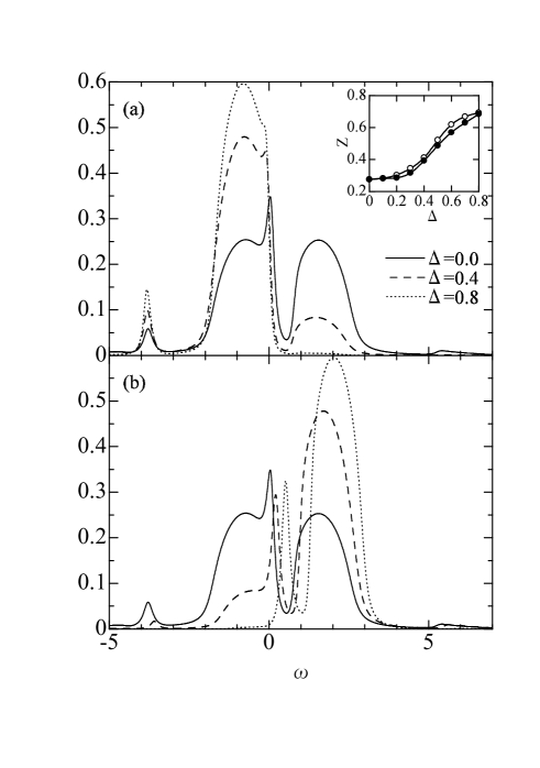
Fig.  5: One-particle spectral function for various values of $\Delta$: $U=2$, $J=0$ and $T=0.1$. The system is close to half filling, $n_{\rm tot}=1.90$. (a) and (b) represent the spectrum for the lower band and the upper band, respectively. The inset shows the renormalization factor for lower band (open circles) and upper band (filled circles).

The overall structure in the spectrum has the shape expected naively. Namely, with the increase of $\Delta$, the weight of the middle peak (doubly occupied state) gets larger and that of the top peak (triply occupied state) becomes smaller in the lower band case (a), while in the upper band case (b), the opposite behavior is observed. It should be noted here that the quasi-particle band disappears gradually with the increase of $\Delta$ and is absorbed into the doubly occupied state. This tendency is different from that observed for quarter filling. Near half-filling, both of the spin fluctuation and the charge fluctuation are suppressed in the presence of $\Delta$, since the lower band is almost fully occupied by electrons of spin singlet. As a result, the system behaves like a renormalized band insulator with both of the spin and charge gaps. Therefore, the formation of heavy electrons is suppressed by $\Delta$ in a metallic phase close to half filling.

The Hund coupling, however, gives rise to a dramatic change in the spectrum in this case. Fig. 6 shows the spectral function for $\Delta=0.8$ in the presence of the Hund coupling.

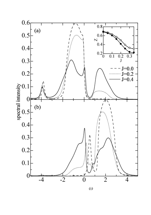
Fig.  6: One-particle spectral function at $U=2$, $\Delta=0.8$ and $T=0.1$. The electron concentration is 1.90 (near half filling). (a) and (b) represent the spectrum for the lower band and the upper band, respectively. The inset shows the renormalization factor for lower band (open circles) and upper band (filled circles).

Although a quasi-particle band around the Fermi level is almost invisible in the absence of the Hund coupling ($J=0$), it is enhanced again with the increase of $J$ in both (a) and (b). In the absence of the Hund coupling, each lattice site is mostly occupied by two electrons of spin singlet in the same orbital. When the Hund coupling is introduced, the energy of the spin-triplet state is lowered, and can be degenerate with the singlet state. This induces the large spin fluctuation, enhancing the quasi-particle mass to form a heavy quasi-particle band. This tendency is clearly seen in the renormalization factor shown in Figs. 5 and 6. As seen in the inset of Fig. 5, when the orbital splitting increases, the renormalization factor for both of the lower (open triangle) and upper bands (filled triangle) increases, while in the inset of Fig. 6 the introduction of the Hund coupling again reduces the renormalization factor. These results imply that the spin fluctuation caused by the Hund coupling enhances the quasi-particle mass in a metallic state near half filling, which is not observed near quarter filling.

3.3 Optical Conductivity

In order to further investigate the dynamical response, we calculate the optical conductivity. We employ the following formula for the optical conductivity,

$$\sigma(\omega)=\pi\sum_{m,\sigma}\int_{-\infty}^{\infty}{\rm d}\epsilon^{\prime}\int_{-\infty}^{\infty}{\rm d}\epsilon\,N_{0}(\epsilon)$$ (3.3)

$$\times A_{m\sigma}(\epsilon,\epsilon^{\prime})A_{m\sigma}(\epsilon,\omega+\epsilon^{\prime})\frac{f(\epsilon^{\prime})-f(\epsilon^{\prime}+\omega)}{\omega},$$

$$A_{m\sigma} (\epsilon,\omega)=-\frac{1}{\pi}{\rm Im}{{\hbox{$\left(\vbox to0.0pt{}\right.\n@space$}}}\frac{1}{\omega+{\rm i}\delta-\epsilon+\mu-\Sigma_{m\sigma}(\omega)}{{\hbox{$\left)\vbox to0.0pt{}\right.\n@space$}}},$$ (3.4)

where the vertex correction is neglected, which is justified in the limit of large dimensions .${}^{\hbox{\immediate{?},\penalty 1000\hskip 0.91003pt plus 0.70004pt minus 0.70004pt{\bf{?}},\penalty 1000\hskip 0.91003pt plus 0.70004pt minus 0.70004pt{?})}}$ The computed results are shown in Fig. 7.

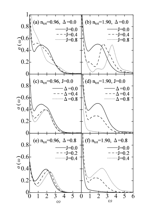
Fig.  7: Optical conductivity $\sigma(\omega)$ for (a) $\Delta=0$ and $n_{\rm tot}=0.96$, (b) $\Delta=0$ and $n_{\rm tot}=1.90$, (c) $J=0$ and $n_{\rm tot}=0.96$, (d) $J=0$ and $n_{\rm tot}=1.90$, (e) $\Delta=0.8$ and $n_{\rm tot}=0.96$, and (f) $\Delta=0.8$ and $n_{\rm tot}=1.90$. The other parameters are $U=2$ and $T=0.10$.

In contrast to the one-particle spectrum, the overall structure of the optical conductivity is not so sensitive to the parameters employed. Nevertheless, we can see some distinct behaviors near quarter filling and half filling. We first discuss the orbitally degenerate case ($\Delta=0$) near quarter filling and half filling shown in Fig. 7 (a) and (b). It is clearly seen both in (a) and (b) for $J=0$ that the optical conductivity consists of the Drude-like part ($\omega\sim 0$) and the interband part. With the increase of $J$ in (a), the weight for the interband absorption gradually shifts to the lower-energy regime, reflecting the splitting of the doubly occupied state due to the Hund coupling, as already shown in Fig. 2 (a). On the other hand in (b) the Drude-like part gets narrower and the interband absorption shifts to the higher-energy part with increase of $J$. This result in (b) reflects that the Hund coupling has a tendency to enhance the charge excitation gap ,${}^{\hbox{\immediate{?})}}$ which is different from the case near quarter filling.

We next discuss the effect of the orbital splitting by observing Fig. 7 (c) and (d), where we assume that the Hund coupling is absent for simplicity. As seen from (c), near quarter filling, the amplitude of the conductivity becomes smaller with the increase of $\Delta$ although the overall structure is almost unchanged. For sufficiently large $\Delta$, the amplitude becomes about half of the case of $\Delta=0$ since the lower band corresponds to that of the single-band model and the upper one exists above the Fermi level ${}^{\hbox{\immediate{?})}}$ (see Fig. 3). On the other hand, the Drude-like peak in (d) becomes narrower while the interband-absorption weight gets smaller as $\Delta$ increases because both of the charge and spin fluctuations are suppressed for large $\Delta$ near half filling, as seen in Fig. 5. Therefore, a slight hole-doping into half-filled band brings about the sharp Drude-like absorption peak in the low energy part.

Finally, we discuss the interplay of the Hund coupling and the orbital splitting. As seen in Fig. 7 (e), the conductivity does not change its characteristic behavior except that the interband absorption slightly shifts to the higher energy regime with the increase of $J$. This is because the Hund coupling hardly affects the low-energy spectrum for large $\Delta$ near quarter filling, since the lower band is reduced to that of the single-band Hubbard model as mentioned in Fig. 5. Near half filling (Fig. 7(f)), however, a rather drastic change occurs in the conductivity: the Drude-like part gets wider and the interband absorption is induced again as $J$ increases, reflecting the appearance of a quasi-particle state near the Fermi level as shown in Fig. 6.

4 Summary and Discussions

We have studied how the interplay of the Hubbard interaction, the Hund coupling and the orbital splitting affects the formation of heavy quasi-particles in the two-orbital Hubbard model. In order to investigate dynamical quantities in the whole energy region, we have exploited dynamical mean field theory with the non-crossing approximation. We have discussed the one-particle spectral function and the optical conductivity for a metallic system in the vicinity of the Mott insulator. In particular, similarity and difference in the formation of heavy quasi-particles between quarter filling and half filling have been clarified. Near quarter filling, hole-doping into the Mott insulator leads to the formation of the heavy quasi-particle band, which is slightly renormalized by the Hund coupling or the orbital splitting. On the other hand, near half filling the orbital splitting prevents the formation of heavy particles, driving to the system to a correlated band-type insulator, for which a heavy quasi-particle band is not formed by hole doping. If the Hund coupling is switched on, however, heavy quasi-particles appear again due to the enhanced spin fluctuation.

In connection with the experimental results for transition metal oxides such as ${\rm La_{1-{\it x}}Sr_{\it x}TiO_{3}}$, ${}^{\hbox{\immediate{?})}}$ the quarter-filled model ($n_{\rm tot}\sim 1$) has been studied extensively. ${}^{\hbox{\immediate{\bf{?}},\penalty 1000\hskip 0.91003pt plus 0.70004pt minus 0.70004pt{\bf{?}},\penalty 1000\hskip 0.91003pt plus 0.70004pt minus 0.70004pt{\bf{?}})}}$ A heavy quasi-particle band studied here was pointed out in a different method, and the overall structure of the one-particle spectrum was quantitatively discussed in comparison with the photoemission experiments,${}^{\hbox{\immediate{\bf{?}})}}$ although a sharp quasi-particle band in the spectrum was not clearly observed experimentally. On the other hand, the half-filled Hubbard model with two orbitals has not been studied systematically thus far in comparison with the quarter-filled model. A possible example in transition metal oxides relevant for this case ($n_{\rm tot}\sim 2$) may be ${\rm La_{1-{\it x}}Sr_{\it x}VO_{3}}$ ${}^{\hbox{\immediate{\bf{?}},\penalty 1000\hskip 0.91003pt plus 0.70004pt minus 0.70004pt{?})}}$ with electron configuration of $3d^{2}$ in V ions. In this material, the Hund coupling forms the $S=1$ spin at each site, resulting in the antiferromagnetic ground state at half filling. According to the results in §3.2 (Fig.4), when holes are doped into this system to realize a paramagnetic metal, a heavy quasi-particle band may not be observed${}^{\hbox{\immediate{?})}}$ because of a rather large Hund-coupling. Nevertheless, we think that for related materials where the orbital splitting due to a crystalline field becomes comparable to the Hund coupling, a heavy quasi-particle formation may be more easily observed experimentally, reflecting the interplay of the above two effects, as pointed out in Fig.6.

References

- [1] M. Imada, A. Fujimori and Y. Tokura: Rev. Mod. Phys. 70 (1998) 1039
- [2] A. C. Hewson: The Kondo Problem to Heavy Fermions (Cambridge Univ. Press, Cambridge 1993)
- [3] M. C. Gutzwiller: Phys. Rev. Lett. 10 (1963) 159
- [4] J. Kanamori: Prog. Theor. Phys. 30 (1963) 235
- [5] J. Hubbard: Proc. Roy. Soc. (London), Ser. A 281 (1964) 401
- [6] W. Metzner and D. Vollhartdt: Phys. Rev. Lett. 62 (1989) 324
- [7] E. Mller-Hartmann: Z. Phys. B 74 (1989) 507; ibid B 76 (1989) 211
- [8] A. George, G. Kotliar, W. Krauth and M. J. Rozenberg: Rev. Mod. Phys. 68 (1996) 13
- [9] Th. Pruschke, D. L. Cox and M. Jarrell: Phys. Rev. B 47 (1993) 3553
- [10] H. Hasegawa: J. Phys. Soc. Jpn. 66 (1997) 1391
- [11] R. Frsard and G. Kotliar: Phys. Rev. B 56 (1997) 12909
- [12] A. Klejnberg and J. Spalek: Phys. Rev. B 57 (1998) 12041
- [13] Y. Motome and M. Imada: J. Phys. Soc. Jpn. 67 (1998) 3199
- [14] G. Kotliar and H. Kajueter : Phys. Rev. B 54 (1996) R14211
- [15] M. J. Rozenberg: Phys. Rev. B 55 (1997) R4855
- [16] J. E. Han, M. Jarrell and D. L. Cox: Phys. Rev. B 58 (1998) R4199
- [17] T. Momoi and K. Kubo: Phys. Rev. B 58 (1998) R567
- [18] P. Lombardo and G. Albinet: cond-mat/0009253
- [19] H. Keiter and J. C. Kimball: Phys. Rev. Lett. 25 (1970) 672
- [20] Y. Kuramoto: Z. Phys. B 53 (1983) 37
- [21] P. Coleman: Phys. Rev. B 29 (1984) 3035
- [22] E. Mller-Hartmann: Z. Phys. B 57 (1984) 281
- [23] N. E. Bickers: Rev. Mod. Phys. 59 (1987) 845
- [24] Th. Pruschke and N. Grewe: Z. Phys. B 74 (1989) 439
- [25] F. J. Ohkawa: J. Phys. Soc. Jpn. 58 (1989) 4156
- [26] A. Khurana: Phys. Rev. Lett. 64 (1990) 1990
- [27] V. I. Anisimov, A. I. Poteryaev, M. A. Korotin, A. O. Anokhin and G. Kotliar: J. Phys.: Condens. Matter 9 (1997) 7359
- [28] M. B. Zlfl, Th. Pruschke, J. Keller, A. I. Poteryaev, I. A. Nekrasov and V. I. Anisimov: Phys. Rev. B 61 (2000) 12810
- [29] I. A. Nekrasov, K. Held, N. Blmer, A. I. Poteryaev, V. I. Anisimov and D. Vollhardt: Euro. Phys. J. B 18 (2000) 55
- [30] A. Fujimori, I. Hase, H. Namatame, Y. Fujishima, Y. Tokura, H. Eisaki, S. Uchida, K. Takegahara and F. M. F. de Groot: Phys. Rev. Lett. 69 (1992) 1796
- [31] F. Inaba, T. Arima, T. Ishikawa, T. Katsufuji and Y. Tokura: Phys. Rev. B 52 (1995) R2221