Critical temperature of SF bilayers Critical temperature of superconductor/ferromagnet bilayers Ya. V. Fominov, N. M. Chtchelkatchev, and A. A. Golubov Fominov, Chtchelkatchev, Golubov 8 June 2001*

Critical temperature of superconductor/ferromagnet bilayers

Abstract

Superconductor/ferromagnet bilayers are known to exhibit nontrivial dependence of the critical temperature $T_{c}$ on the thickness $d_{f}$ of the ferromagnetic layer. We develop a general method for investigation of $T_{c}$ as a function of the bilayer’s parameters. It is shown that interference of quasiparticles makes $T_{c}(d_{f})$ a nonmonotonic function. The results are in good agreement with experiment. Our method also applies to multilayered structures.

74.50.+r, 74.80.Dm, 75.30.Et

Recently, much attention has been paid to properties of hybrid proximity systems containing superconductors (S) and ferromagnets (F); new physical phenomena were predicted and observed in these systems [1, 2, 3, 4]. One of the most striking effects in SF layered structures is highly nonmonotonic dependence of the critical temperature $T_{c}$ of the system on the thickness $d_{f}$ of the ferromagnetic layers. Experiments exploring this nonmonotonic behavior have been performed previously on SF multilayers such as Nb/Gd [5], Nb/Fe [6], V/V-Fe [7], and Pb/Fe [8] but the results (and, in particular, comparison between the experiments and theories) were not conclusive.

To perform reliable experimental measurements of $T_{c}(d_{f})$, it is essential to have $d_{f}$ large compared to the interatomic distance; this situation can be achieved only in the limit of weak ferromagnets. Active experimental investigations of SF bilayers and multilayers based on Cu-Ni dilute ferromagnetic alloys are carried out by the group of Ryazanov [9]. In SF bilayers, they observed highly nonmonotonic dependence $T_{c}(d_{f})$. While the reason for this effect in multilayers can be the $0$–$\pi$ transition [3], in a bilayer system with a single superconductor this mechanism is irrelevant and the cause of the effect is quasiparticle interference specific to SF structures.

In the present paper, motivated by the ROP experiment [9] we study theoretically the critical temperature of SF bilayers. Previous theoretical investigations of $T_{c}$ in SF structures were concentrated on systems with thin or thick S(F) layers [compared to the coherence length of the superconductor (ferromagnet)]; with SF boundaries having very low or very high transparency; besides, the exchange energy was often assumed to be much larger then the critical temperature [3, 7, 8, 10, 11, 12, 13]. The parameters of the ROP experiment do not correspond to any of these limiting cases. In the present paper we develop an approach giving opportunity to investigate not only the limiting cases of parameters, but also the intermediate region. Using our method, we find different types of nonmonotonic behavior of $T_{c}$ as a function of $d_{f}$ such as minimum of $T_{c}$ and even reentrant superconductivity [14]. Comparison of our theoretical predictions with the experimental data shows good agreement.

We assume that dirty-limit conditions are fulfilled, and calculate the critical temperature of the bilayer within the framework of the linearized Usadel equations for S and F layers (the domain $0<x<d_{s}$ is occupied by the S metal, $-d_{f}<x<0$ — by the F metal, see Fig.1). Near $T_{c}$ the normal Green function is $G=\operatorname{sgn}\omega_{n}$, and the Usadel equations for the anomalous function $F$ take the form:

$$\xi_{s}^{2}\,\pi T_{cs}\frac{d^{2}F_{s}}{dx^{2}}-|\omega_{n}|F_{s}+\Delta=0,\quad 0<x<d_{s};$$ (1)

$$\xi_{f}^{2}\,\pi T_{cs}\frac{d^{2}F_{f}}{dx^{2}}-(|\omega_{n}|+iE_{\mathrm{ex}}\operatorname{sgn}\omega_{n})F_{f}=0,$$ (2)

$$-d_{f}<x<0;$$

$$\Delta\ln\frac{T_{cs}}{T}=\pi T\sum_{\omega_{n}}\left(\frac{\Delta}{|\omega_{n}|}-F_{s}\right),$$ (3)

where $\xi_{s}=\sqrt{D_{s}/2\pi T_{cs}}$, $\xi_{f}=\sqrt{D_{f}/2\pi T_{cs}}$, $\omega_{n}=\pi T(2n+1)$ with $n=0,\pm 1,\pm 2,\ldots$ are the Matsubara frequencies, $E_{\mathrm{ex}}$ is the exchange energy, and $T_{cs}$ is the critical temperature of the S layer. $F_{s(f)}$ denotes the function $F$ in the S(F) region.

Equations (1)-(3) must be supplemented with the boundary conditions at the outer surfaces of the bilayer:

$$\frac{dF_{s}(d_{s})}{dx}=\frac{dF_{f}(-d_{f})}{dx}=0,$$ (4)

as well as at the SF boundary:

$$\xi_{s}\frac{dF_{s}(0)}{dx}=\gamma\xi_{f}\frac{dF_{f}(0)}{dx}, \gamma=\frac{\rho_{s}\xi_{s}}{\rho_{f}\xi_{f}},$$ (5)

$$\xi_{f}\gamma_{b}\frac{dF_{f}(0)}{dx}=F_{s}(0)-F_{f}(0), \gamma_{b}=\frac{R_{b}{\cal A}}{\rho_{f}\xi_{f}}.$$ (6)

Here $\rho_{s,f}$ are the normal state resistivities of the S and F metals, $R_{b}$ is the total resistance of the SF boundary, and ${\cal A}$ is its area. The Usadel equation in the F layer is readily solved:

$$F_{f}=C(\omega_{n})\cosh\left(k_{f}(x+d_{f})\right),$$ (7)

$$\text{with }k_{f}=\frac{1}{\xi_{f}}\sqrt{\frac{|\omega_{n}|+iE_{\mathrm{ex}}\operatorname{sgn}\omega_{n}}{\pi T_{cs}}},$$ (8)

and the boundary condition at $x=0$ can be written in closed form with respect to $F_{s}$:

$$\xi_{s}\frac{dF_{s}(0)}{dx}=\frac{\gamma}{\gamma_{b}+B_{f}(\omega_{n})}F_{s}(0),$$ (9)

where $B_{f}(\omega_{n})=\left[k_{f}\xi_{f}\tanh(k_{f}d_{f})\right]^{-1}$.

This boundary condition is complex. In order to rewrite it in real form, we do the usual trick and go over to the functions $F^{\pm}=F(\omega_{n})\pm F(-\omega_{n})$. The symmetric properties of $F^{+}$ and $F^{-}$ are trivial, so we will treat only positive $\omega_{n}$. The self-consistency equation is expressed only via the symmetric function $F_{s}^{+}$:

$$\Delta\ln\frac{T_{cs}}{T}=\pi T\sum_{\omega_{n}>0}\left(\frac{2\Delta}{\omega_{n}}-F_{s}^{+}\right),$$ (10)

and the problem of determining $T_{c}$ can be formulated in closed form with respect to $F_{s}^{+}$. This is done as follows. The Usadel equation for $F_{s}^{-}$ does not contain $\Delta$, hence it can be solved analytically. After that we exclude $F_{s}^{-}$ from the boundary condition (9) and arrive at the effective boundary conditions for $F_{s}^{+}$:

$$\xi_{s}\frac{dF_{s}^{+}(0)}{dx}=W(\omega_{n})F_{s}^{+}(0),\qquad\frac{dF_{s}^{+}(d_{s})}{dx}=0,$$ (11)

where

$$W=\gamma\frac{A_{s}(\gamma_{b}+\Real B_{f})+\gamma}{A_{s}|\gamma_{b}+B_{f}|^{2}+\gamma(\gamma_{b}+\Real B_{f})},$$ (12)

$$A_{s}=k_{s}\xi_{s}\tanh(k_{s}d_{s}),\quad\text{with }k_{s}=\frac{1}{\xi_{s}}\sqrt{\frac{\omega_{n}}{\pi T_{cs}}}.$$

The self-consistency equation (10), the boundary conditions (11)-(12) together with the Usadel equation for $F_{s}^{+}$:

$$\xi_{s}^{2}\,\pi T_{cs}\frac{d^{2}F_{s}^{+}}{dx^{2}}-\omega_{n}F_{s}^{+}+2\Delta=0$$ (13)

will be used below to find the critical temperature of the bilayer.

The Green function (in mathematical sense) of the problem (11)–(13) can be expressed via solutions $v_{1}$, $v_{2}$ of Eq. (13) without $\Delta$, satisfying the boundary conditions at $x=0$ and $x=d_{s}$, respectively:

$$G(x,y;\omega_{n})=\frac{k_{s}\xi_{s}/\omega_{n}}{\sinh(k_{s}d_{s})+a\cdot\cosh\left(k_{s}d_{s}\right)}\times\\ \times\left\{\begin{aligned} v_{1}(x)v_{2}(y),&&x\leq y\\ v_{2}(x)v_{1}(y),&&y\leq x\end{aligned}\right.,$$ (14)

where $a=W(\omega_{n})/k_{s}\xi_{s}$ and

$$v_{1}(x) =\cosh(k_{s}x)+a\cdot\sinh(k_{s}x),$$

$$v_{2}(x) =\cosh\left(k_{s}(x-d_{s})\right).$$ (15)

Having found $G(x,y;\omega_{n})$, we can write the solution of Eqs. (11)–(13) as

$$F_{s}^{+}(x;\omega_{n})=2\int_{0}^{d_{s}}G(x,y;\omega_{n})\Delta(y)dy.$$ (16)

Substituting this into the self-consistency equation (10), we obtain

$$\Delta(x)\ln\frac{T_{cs}}{T_{c}}=\\ =2\pi T_{c}\sum_{\omega_{n}>0}\left[\frac{\Delta(x)}{\omega_{n}}-\int_{0}^{d_{s}}G(x,y;\omega_{n})\Delta(y)dy\right].$$ (17)

This equation can be expressed in symbolic form: $\Delta\ln(T_{cs}/T_{c})=\hat{L}\Delta$. Then $T_{c}$ is determined from the condition

$$\det\left(\hat{L}-\hat{1}\ln\frac{T_{cs}}{T_{c}}\right)=0$$ (18)

that Eq. (17) has a nontrivial solution with respect to $\Delta$. Numerically, we put our problem (17)–(18) on the spatial grid so that the linear operator $\hat{L}$ becomes a finite matrix.

Equations (14)–(18) are our central result; substituting the concrete parameters of the system we can easily find the critical temperature numerically and in certain cases analytically. (The models considered previously [3, 7, 8, 10, 11, 12, 13] correspond to the limiting cases of our theory.)

We apply our method to fit the ROP experimental data [9]; the result is presented in Fig.2. Estimating the parameters $d_{s}=11$ nm, $T_{cs}=7$ K, $\rho_{s}=7.5$ $\mu\Omega$ cm, $\xi_{s}=8.9$ nm, $\rho_{f}=60$ $\mu\Omega$ cm, $\xi_{f}=7.6$ nm, $\gamma=0.15$ from the experiment and fitting only $E_{\mathrm{ex}}$ and $\gamma_{b}$, we find good agreement between our theoretical predictions and the experimental data. The fitting procedure was the following: first, we determine $E_{\mathrm{ex}}\approx 130$ K from the position of the minimum of $T_{c}(d_{f})$; second, we find $\gamma_{b}\approx 0.3$ from fitting the vertical position of the curve. The deviation of our curve from the experimental points is small; it is most pronounced in the region of small $d_{f}$ corresponding to the initial decrease of $T_{c}$. This is not unexpected because when $d_{f}$ is of the order of a few nanometers, the thickness of the F film may vary significantly along the film (which is not taken into account in our theory) and the thinnest films can even be formed by an array of islands rather then by continuous material. At the same time, we note that the minimum of $T_{c}$ takes place at $d_{f}\approx 5$ nm, when with good accuracy the F layer has uniform thickness.

The position of the minimum of $T_{c}(d_{f})$ can be estimated from qualitative arguments based on interference of quasiparticles in the ferromagnet. Let us consider a point $x$ inside the F layer. According to Feynman’s interpretation of quantum mechanics [15], the quasiparticle wave function [we are interested in anomalous wave function of correlated quasiparticles, which characterizes the superconductivity; this function is equivalent to the anomalous Green function $F(x)$] may be represented as a sum of the wave amplitudes over all classical trajectories; the wave amplitude for a given trajectory equals $\exp(iS)$, where $S$ is the classical action along this trajectory. To obtain our anomalous wave function we must sum over trajectories that (i) start and end at the point $x$, (ii) change the type of the quasiparticle (i.e., convert an electron into a hole or vice versa). There are four kinds of trajectories which should be taken into account (see Fig.1). Two of them (denoted 1 and 2) start in the direction toward the SF interface (as an electron and as a hole), experience the Andreev reflection and return to the point $x$. The other two trajectories (denoted 3 and 4) start in the direction away from the interface, experience normal reflection at the outer surface of the F layer, move toward the SF interface, experience the Andreev reflection there, and finally return to the point $x$. The main contribution is given by the trajectories normal to the interface. The corresponding actions are $S_{1}=-S_{2}=-Qx$ and $S_{3}=-S_{4}=-Q(2d_{f}+x)$ (note that $x<0$), where $Q$ is the difference between the wave numbers of the electron and the hole. To make our arguments more clear, we assume that the ferromagnet is strong, the SF interface is ideal, and consider the clean limit first: in this case $Q=k_{e}-k_{h}=\sqrt{2m(E+E_{\mathrm{ex}}+\mu)}-\sqrt{2m(-E-E_{\mathrm{ex}}+\mu)}\approx 2E_{\mathrm{ex}}/v$, where $E$ is the quasiparticle energy, $\mu$ is the Fermi energy, and $v$ is the Fermi velocity. Thus the anomalous wave function of the quasiparticles is $F(x)\propto\sum_{n=1}^{4}\exp(iS_{n})\propto\cos(Qd_{f})\cos(Q(d_{f}+x))$. The suppression of $T_{c}$ by the ferromagnet is determined by the value of the wave function at the SF interface: $F(0)\propto\cos^{2}(Qd_{f})$. The minimum of $T_{c}$ corresponds to the minimal value of $F(0)$ which is achieved at $d_{f}=\pi/2Q$. In the dirty limit the above expression for $Q$ is replaced by $Q=\sqrt{E_{\mathrm{ex}}/D_{f}}$, hence the minimum of $T_{c}(d_{f})$ takes place at

$$d_{f}^{\rm(min)}=\frac{\pi}{2}\sqrt{\frac{D_{f}}{E_{\mathrm{ex}}}}.$$ (19)

In the case of the ROP bilayer [9] we obtain $d_{f}^{\rm(min)}\approx 7$ nm, whereas the experimental value is $5$ nm (Fig.2); thus our qualitative estimate appears to be reasonable.

The method developed in this paper applies directly to multilayered SF structures (in particular, to trilayers) in the $0$-state, where an SF bilayer can be considered as an elementary cell of the system. A generalization can be made, which allows to take account of possible superconductive and/or magnetic $\pi$-states.

In conclusion, we have developed a method for calculating the critical temperature of a SF bilayer as a function of parameters of the junction. The approach developed here gives an opportunity to evaluate $T_{c}$ in wide range of parameters. We demonstrate that there is good agreement between the experimental data and our theoretical predictions. Qualitative arguments are given, which explain the nonmonotonic behavior of the function $T_{c}(d_{f})$. Extensive details of our study will be published elsewhere [14].

We thank V. V. Ryazanov and M. V. Feigel’man for stimulating discussions and useful comments on the manuscript. We are especially indebted to V. V. Ryazanov for communicating the experimental result of his group to us prior to the detailed publication. Also we are grateful to M. Yu. Kupriyanov and Yu. Oreg for enlightening comments. Ya.V.F. acknowledges financial support from the Russian Foundation for Basic Research (RFBR), project No. 01-02-17759, and from Forschungszentrum Jülich (Landau Scholarship). The research of N.M.C. was supported by the RFBR, project No. 01-02-06230, by Forschungszentrum Jülich (Landau Scholarship), by the Netherlands Organization for Scientific Research (NWO), and by the Swiss National Foundation.

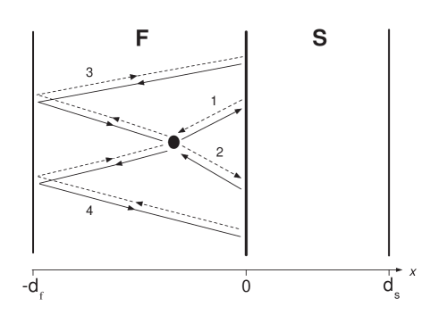
Figure 1:

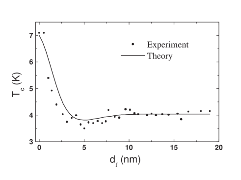
Figure 2:

Fig.1. The SF bilayer. The F and S layers occupy the regions $-d_{f}<x<0$ and $0<x<d_{s}$, respectively. The four types of trajectories contributing (in Feynman path integral sense) to the anomalous wave function of correlated quasiparticles are shown in the ferromagnetic region. The solid lines correspond to electrons, the dashed lines — to holes; the arrows indicate the direction of the velocity.

Fig.2. Theoretical fit to ROP’s experimental data [9]. In the experiment, Nb was the superconductor (with $d_{s}=11$ nm, $T_{cs}=7$ K) and Cu_0.43Ni_0.57 was the weak ferromagnet. From our fit we estimate $E_{\mathrm{ex}}\approx 130$ K and $\gamma_{b}\approx 0.3$.

References

- [1] V. V. Ryazanov, V. A. Oboznov, A. Yu. Rusanov et al., Phys. Rev. Lett. 86, 2427 (2001); V. V. Ryazanov, V. A. Oboznov, A. V. Veretennikov et al., cond-mat/0103240.
- [2] T. Kontos, M. Aprili, J. Lesueur et al., Phys. Rev. Lett. 86, 304 (2001).
- [3] Z. Radović, M. Ledvij, Lj. Dobrosavljević–Grujić et al., Phys. Rev. B 44, 759 (1991).
- [4] L. R. Tagirov, Phys. Rev. Lett. 83, 2058 (1999).
- [5] J. S. Jiang, D. Davidović, D. H. Reich et al., Phys. Rev. Lett. 74, 314 (1995).
- [6] Th. Mühge, N. N. Garif’yanov, Yu. V. Goryunov et al., Phys. Rev. Lett 77, 1857 (1996).
- [7] J. Aarts, J. M. E. Geers, E. Brück et al., Phys. Rev. B 56, 2779 (1997).
- [8] L. Lazar, K. Westerholt, H. Zabel et al., Phys. Rev. B 61, 3711 (2000).
- [9] V. V. Ryazanov, V. A. Oboznov, A. S. Prokof’ev et al., to be published.
- [10] A. I. Buzdin, B. Vujičić, and M. Yu. Kupriyanov, Zh. Eksp. Teor. Fiz. 101, 231 (1992) [Sov. Phys. JETP 74, 124 (1992)].
- [11] E. A. Demler, G. B. Arnold, and M. R. Beasley, Phys. Rev. B 55, 15174 (1997).
- [12] Yu. N. Proshin and M. G. Khusainov, Zh. Eksp. Teor. Fiz. 113, 1708 (1998) [Sov. Phys. JETP 86, 930 (1998)]; 116, 1887 (1999) [89, 1021 (1999)].
- [13] L. R. Tagirov, Physica C 307, 145 (1998).
- [14] Ya. V. Fominov, N. M. Chtchelkatchev, and A. A. Golubov, in preparation.
- [15] R. P. Feynman and A. R. Hibbs, Quantum Mechanics and Path Integrals (McGraw-Hill, New York, 1965).