Theory of the Quantum Hall Smectic Phase, II: Microscopic Theory

Abstract

We present a microscopic derivation of the hydrodynamic theory of the Quantum Hall smectic or stripe phase of a two-dimensional electron gas in a large magnetic field. The effective action of the low energy is derived here from a microscopic picture by integrating out high energy excitations with a scale of the order the cyclotron energy. The remaining low-energy theory can be expressed in terms of two canonically conjugate sets of degrees of freedom: the displacement field, that describes the fluctuations of the shapes of the stripes, and the local charge fluctuations on each stripe.

I Introduction

It is by now generally accepted that electron correlations in a 2DEG at sufficiently high Landau levels, are responsible for the large anisotropies in the transport properties observed in recent experiments on extremely high mobility samples in large magnetic fieldsLilly ; du ; subsequent . Analyzing fluctuations around a Hartree-Fock stripe state platzman ; fogler ; chalker ; tudor , and exploiting an analogy with the stripe related phases of other strongly correlated electron systemsnature , Fradkin and Kivelson proposed FK that the ground states of Quantum Hall Systems with partially filled Landau levels with $N\geq 2$ are predominantly electronic liquid crystalline.

In a separate paper, coauthored with S. A. Kivelson and V. Oganesyan BFKO , hereafter referred to as paper I, we proposed an effective low-energy theory for the Quantum Hall Smectic described in terms of the Goldstone modes of the broken translation and rotation symmetry. The effective low energy Lagrangian for this state is given by

$${\cal L}=\frac{eB}{\lambda}u\partial_{t}\phi-\frac{\kappa_{\parallel}}{2}(\partial_{x}\phi)^{2}-\frac{\kappa_{\perp}}{2}(\partial_{y}u)^{2}-\frac{Q}{2}(\partial_{x}^{2}u)^{2}.$$ (1)

where we have assumed that the stripes run along the $x$ direction. Here $u(x,y)$ is the displacement field, the Goldstone mode of the broken translation symmetry, representing the transverse displacements of the stripes (i. e. along the $y$ direction); $\phi$ is the Luttinger field, representing the charge fluctuations on each stripe; $\lambda$ is the wavelength of the stripe state; $\kappa_{\parallel}$, $\kappa_{\perp}$ and $Q$ are elastic constants.

In this paper we give a physically intuitive microscopic derivation of the effective low-energy theory of Eq. 1. The approach that we will use here is based on a microscopic theory which focuses on the role of dynamical shape fluctuations in the quantum Hall stripe state and to their coupling with the charge fluctuations in this state. Thus, we will pay special attention to the role played by the displacement field $u$, as well as to its coupling to the charge fluctuations on each stripe represented by the Luttinger field $\phi$.

The construction that we use here is partially inspired by the picture of the quantum Hall smectic suggested by Hartree-Fock calculationsplatzman ; fogler ; chalker ; tudor ; fertig ; fertig-stability ; fertig-cote . Koulakov and coworkersfogler and Moessner and Chalkerchalker found that the stripe state can be viewed as a set of $N$ filled Landau levels, with a charge modulation due to the electrons in the partially filled Landau level (see figure 1). For fully polarized (“spinless”) fermions at a static level this state looks like an array of strips of charge, corresponding to regions with an effective filling factor $N+1$, surrounded by regions with filling factor $N$. Thus, the electrons arrange themselves in a state which locally mimics a gapped integer Hall state. If this charge-modulated state was due to an imposed external potential, inside these regions the electron fluid would be incompressible and only the excitations at their “edges” would remain gapless. Hence, at a static level, the state looks like an array of fixed chiral Luttinger liquids, the edges of integer quantum Hall stripes, a picture advocated by Fradkin and Kivelson FK , and by MacDonald and FisherMF (see also ref. EFKL ; carpentier ). This, however, is not the full story since this charge modulated state is a self-consistent ground state, and not the result on any externally applied potential.

In an insightful paper, MacDonald and Fisher investigated the properties of the quantum Hall smectic viewed as an array of coupled chiral Luttinger liquids subject to constraints imposed by the requirement of global rotational invariance. One of the issues raised in ref. MF is how many independent degrees of freedom does the quantum Hall smectic actually have. Fradkin and KivelsonFK had advocated a picture in which both charge and shape degrees of freedom although coupled were both part of the physical picture. Direct inspection of the effective action of Eq. 1 shows that the displacement field $u$, which embodies the shape fluctuations, and the Luttinger field $\phi$ of charge fluctuations are canonically conjugate dynamical variable much as coordinates and momenta are in Classical Mechanics. This connection is a direct manifestation of the Lorentz force, crucial for the dynamics of charged particles in magnetic fields. Thus, although shape and charge are both useful descriptions of the physics, we find that they are not truly independent degrees of freedom, in agreement with the point of view of MacDonald and Fisher.

A simple change of basis relates the quantum smectic picture, which uses as degrees of freedom the displacement field $u$ and the Luttinger field $\phi$, and the picture of an array of coupled chiral Luttinger liquids:

$$u \to \partial_{x}\phi^{+}+\partial_{x}\phi^{-}$$ (2)

$$\phi \to \phi^{+}-\phi^{-}$$ (3)

In the chiral Luttinger liquid basis the effective Lagrangian of Eq. (1) theory takes the same form as in the effective theory of MacDonald and FisherMF .

Figure 1: Schematic representation of the quantum Hall smectic state as a set of stripes, running along the vertical $x$ axis. Here $N+\nu^{*}$ is the total filling factor, $\lambda$ is the period of the stripe, $\phi(y)$ is the effective local potential and $\mu$ is the effective chemical potential. The arrows represent the internal chiral edge states.

In Hartree-Fock theories of the stripe statefogler ; chalker ; fertig ; fertig-cote ; fertig-stability ; tudor , the stripe state is derived by balancing the energy density of the Hartree contribution, which favors phase separation, against the energy density of the Fock contribution which, as an exchange driven effect favors the spreading out of the charge. In these calculations, Landau level mixing is taken into account in the form of an effective interaction for electrons in a partially filled Landau level but it is otherwise ignored.The resulting stripe state is structure with a fairly short wavelength $\lambda$. For Landau level index $N=2$, Hartree-Fock calculations yield a wavelength $\lambda\sim 3\ell$, where $\ell$ is the magnetic length, whereas for $N\gg 1$, Moessner and Chalker find chalker $\lambda\sim\textrm{const.}\;\sqrt{N}\ell$, where the constant factor is a number of order $3$. At the level of these calculations fogler ; chalker dynamics is ignored. Dynamics is incorporated later on, at the level of a time-dependent Hartree-Fock approximation, as in the extensive work of Fertig and coworkers fertig-cote ; fertig-stability . Using these methods Fertig and coworkers calculated the spectrum of collective modes, and studied the problem of the stability of the stripe state with respect to a possible stripe crystal. However, while Hartree-Fock theories have been very successful in predicting a smectic state and in studying some of its important properties, they do not yield a transparent picture of the role of the quantum fluctuations of the edges of the charge stripes. Conceptually, this is an undesirable feature since the displacement fields of these edges are the Goldstone bosons of the spontaneously broken translation symmetry.

The main purpose of this paper is to construct an effective theory in which the effects and the dynamics of the displacement field $u$, the Goldstone boson of the broken translation symmetry of the quantum Hall smectic, and of the Luttinger field $\phi$, is made explicit. Although it is possible to derive the effective theory by a detailed analysis of a Hartree-Fock calculation, as was done by Lopatnikova and coworkersbert recently and independently from this work, here we will introduce instead an alternative approach based on the intuitive picture of the stripe state as an array of regions of integer quantum Hall states separated by dynamical edges. For simplicity we will consider the case of short range interactions with a pair potential given in Eq. 11, instead of a long range Coulomb interaction. Although long range interactions change the behavior of the charged collective modes, their precise form are not central neither to the existence of the stripe state itself nor to much (but not all) of the qualitative physics.

We begin by constructing an effective local potential by means of a decoupling of the microscopic density-density interactions in terms of a Hubbard-Stratonovich field $\varphi$, and then proceeding to (formally) integrating out the fermionic degrees of freedom. At the level of a static approximation, the field $\varphi$ plays essentially the role of a scalar (Hartree) potential self-consistently generated by the electron-electron interactions. For a system of electrons in a fixed area, the Hartree term leads to a phase-separation instability. As we pointed out above, the exchange effects of the Fock term stabilize a stripe structure. We will show here that it is possible to stabilize the stripe state instead by the quantum fluctuations of the edge states and by a suitable choice of boundary conditions. Below we construct an effective action which includes the effects of the Hartree contributions and of the quantum fluctuations of the edge states and show that this action leads to a stable stripe solution provided we choose boundary conditions with a fixed number of stripe wavelengths. The resulting stripe state that we find has a wavelength comparable in scale to the wavelength found by Hartree-Fock calculations fogler ; chalker , but the ground state energy is not as good. (Naturally, it is possible to compute the effects of the Fock terms.) Nevertheless, the approach use here leads to an effective action parametrized instead by the geometry of the stripe states, i. e. the positions of the stripes (or “internal edges”), and by the local charge fluctuations on each stripe. Furthermore, we also find that the elastic constants of the effective theory are physically sensible.

The next step is to construct the stripe ground state as a solution of the saddle-point (self-consistent) equations derived from an effective action as described above. We will assume that the stripe state locally looks like regions of a integer quantum Hall states separated by edges. We then construct the stripe solution with a fixed integer number $n$ of periods of wavelength $\lambda$ for the stripe for a geometry of width $L_{y}=n\lambda$. We will then compute the total energy of this state with a fixed number of periods. This total energy has two contributions: (a) a piece coming from the “bulk regions” and (b) a piece coming from the “edges”. We will then find the optimal solution by minimizing the total energy as the period $\lambda$ is varied while keeping the number of periods $n$ fixed.

The saddle-point solution thus constructed, $\varphi_{sp}$, is a smooth differentiable function of the coordinate $y$ normal to the stripe orientation. It varies periodically in space about an average value which plays the role of the Fermi energy. The plane is thus split into two types of regions: (a) regions in which the field $\varphi_{sp}$ is nearly constant and far from the Fermi energy, (b) and regions in which $\varphi_{sp}$ crosses the Fermi energy. In the former, the system behaves as a perturbed Landau level problem with a full gap in the single particle spectrum. Inside these regions we can approximate the effective action for slow time and space dependent fluctuations of $\varphi$ by means a gradient expansion of the fermionic determinant. In other terms, we will keep field configurations which vary slowly on the scale of the cyclotron gap and are smooth on scales long compared with the cyclotron length. This procedure is safe away from edge states. However, wherever $\varphi_{sp}$ crosses the Fermi level, the system has gapless fermionic excitations. In these regions it behaves like an edge state with a definite Fermi velocity determined by the slope of the stripe solution. These edge states regions must be taken into account explicitly in order stabilize the stripe state. (These approximations are very accurate if the wavelength of the stripe state is long compared to the cyclotron length. However, for reasonable interactions it is not the case. Nonetheless we will work within this approximation since it yields qualitatively correct answers.)

Thus, instead of regarding the edges as quasi-static structures, the quantum Hall smectic is a theory of fermions moving on fluctuating stripes. This motion of the stripes is physically due to the fact that the position of the stripes is defined arbitrarily (up to a displacement by an integer number of wavelengths). This arbitrariness is due to the fact that the translation symmetry normal to the stripe is spontaneously broken in this state. Since this is a continuous symmetry, there should be a Goldstone boson associated with it, which we will parametrize by the displacement field $u$ of the stripe position. In other terms, a correct quantum theory of this state requires that these collective modes be quantized correctly. We will do this by parametrizing the physically important configurations as deformed stripe solutions $\varphi_{sp}$ of the form

$$\varphi_{sp}=\varphi_{sp}\left(y\sqrt{1-\frac{1}{2}(\partial_{x}u)^{2}}+u\right)$$ (4)

where $u=u(x,y,t)$ is the displacement field. Hence, we will describe the fluctuations of the quantum hall smectic in terms of two sets of degrees of freedom: (a) the “internal” chiral fermions and (b) the shape fluctuations represented by a dynamical displacement field. Nevertheless, we will see below that these degrees of freedom are not independent from each other and that they are related in a manner dictated entirely by the quantum mechanics of a charged fluid in a magnetic field.

This paper is organized as follows. In Section II we present the derivation of the effective action for the stripe state. Here we construct an effective action for $\varphi$ in the “bulk regions” and at long wavelengths, and show how it couples to the edge modes. These in turn will be written in terms of a set of chiral edge bosons. We will use this effective action to find the optimal stripe solution of the saddle-point equations, which is presented in Section III. In this section, and in Appendix A, we discuss how the (Hartree) stripe solution is stabilized by quantum edge fluctuations. It turns out that the results that follow from the solution that we will derive here has the same physical properties and it is for all practical purposes equivalent to the results of the Hartree-Fock theories. In Section IV we analyze the effect of quantum fluctuations around the saddle-point. Here we derive the coupling between the displacement field $u$ and the non-chiral Luttinger field $\phi$. In this section we give an estimate of the elastic constants entering in Eq. (1). Finally, in Section V we discuss our results and present our conclusions. In the Appendices we give technical details of the derivations discussed in the text.

II Effective action for the quantum Hall stripe state

In this section we will derive an effective action well suited for description of an inhomogeneous state such as a stripe state. Thus we will begin with a microscopic theory of interacting electrons in a large magnetic field and identify the degrees of freedom needed to construct a stripe state. In section III we will find the optimal stripe solution by means of a variational approach.

The generating functional of two-dimensional (non-relativistic) interacting fully spin-polarized electrons in a perpendicular magnetic field is

$$Z[{\tilde{A}}_{\mu}]=\int{\cal D}\psi^{*}{\cal D}\psi~{}e^{iS(\psi,{\tilde{A}}_{\mu})}$$ (5)

where

$$S = \int d^{3}z~{}\left[\psi^{*}(z)[iD_{0}-\mu]\psi(z)+\frac{1}{2m}\left|{\bf D}\psi(z)\right|^{2}\right]$$ (6)

$$- \frac{e^{2}}{2}\int d^{3}zd^{3}z^{\prime}~{}|\psi(z)|^{2}V(z-z^{\prime})|\psi(z^{\prime})|^{2}$$

and

$$D_{\mu}=\partial_{\mu}+ieA_{\mu}+ie{\tilde{A}}_{\mu}$$ (7)

is the covariant derivative. Here $\vec{\nabla}\times\vec{A}={\vec{B}}$ is the external uniform magnetic field, $V(x-y)$ is a two-body interaction potential and ${\tilde{A}}_{\mu}$ are small electromagnetic perturbations introduced to probe the system.

We can decouple the quartic interaction term by means of a Hubbard-Stratonovich (HS) transformation, and introduce a new field $\varphi$. The generating functional now takes the form,

$$Z[{\tilde{A}}_{\mu}]=\int{\cal D}\psi^{*}{\cal D}\psi{\cal D}\varphi~{}e^{iS[\psi,{\tilde{A}}_{\mu},\varphi]}$$ (8)

with

$$S = \int d^{3}z~{}\left[\psi^{*}(z)[iD_{0}-\mu-\varphi]\psi(z)+\frac{1}{2m}\left|{\bf D}\psi(z)\right|^{2}\right]$$ (9)

$$+ \frac{1}{2}\int d^{3}z\int d^{3}z^{\prime}~{}\varphi(z)V^{-1}(z-z^{\prime})\varphi(z^{\prime})$$

where $V^{-1}$ is the inverse of the instantaneous pair potential operator $V(z-z^{\prime})$. Much of what we will discuss here can be done for any pair potential. However, to be able to find an explicit analytic solution we will work with a short range interaction with coupling constant $g$ and range $a$. In any event at this level the physics will not depend too much on the details of the pair interaction. In particular, there exists a choice of short range pair interactions for which the contribution of the interaction term to the action reduces to the following local expression:

$$\frac{1}{2}\int\;d^{3}x\int\;d^{3}x^{\prime}\;\varphi(x)V^{-1}(x-x^{\prime})\varphi(x^{\prime})$$ (10)

$$\equiv\int d^{3}x\;\left(\;{\frac{a^{2}}{2g}}\left(\nabla\varphi(x)\right)^{2}+{\frac{1}{2g}}\varphi(x)^{2}\right)$$

provided that $V(\vec{x})$ is the short ranged interaction potential

$$V({\vec{x}})={\frac{g}{2\pi a^{2}}}K_{0}\left({\frac{|{\vec{x}}|}{a}}\right)$$ (11)

where $K_{0}(z)$ is the modified Bessel function.

The fermionic action is now quadratic and, formally, the fermionic path integral can be carried out obtaining

$$Z({\tilde{A}}_{\mu})=\int{\cal D}\varphi e^{iS_{\rm eff}[{\tilde{A}}_{\mu},\varphi]}$$ (12)

where $S_{\rm eff}({\tilde{A}}_{\mu}\varphi)$ is given by

$$S_{\rm eff} = -i{\rm Tr}\ln\left[iD_{0}-\mu-\varphi+\frac{1}{2m}{\bf D}^{2}\right]$$ (13)

$$+ \frac{1}{2}\int d^{3}zd^{3}z^{\prime}~{}\varphi(z)V^{-1}(z-z^{\prime})\varphi(z^{\prime})$$

This effective action is well defined provided the fermion determinant does not have any zero eigenvalues. However, even for fairly general smooth configurations of the field $\varphi$ there can be zero modes in the fermion determinant. To see this, let us consider configurations in which $\varphi$ varies very slowly. In this case, the main effect of the field $\varphi$ is to shift the single particle energies of the electrons, i. e. the energies of the Landau levels will vary from point to point but sufficiently slowly so that Landau level mixing can be ignored to a first approximation. Thus, at least locally in space, the electrons fill up an integer number $N$ of Landau levels. Clearly, the Hubbard-Stratonovich field $\varphi$ plays the role of an effective local chemical potential. Thus, almost everywhere in space, for these field configurations there is a gap in the fermionic spectrum of the order of the cyclotron energy, $\hbar\omega_{c}$. In this case, the fermion determinant is well behaved. It is well known that, for such regular configurations, the effective action, $S_{\rm bulk}$, is a local functional of $\varphi$ and its derivativessakita ; hosotani ; salam ; LF ; BLA . However, where $\varphi$ crosses the Fermi energy, i.e. where the number of filled Landau levels changes from $N$ to $N-1$, the gap vanishes, there are fermion zero modes, and hence the fermion determinant is badly behaved. The points of the plane where, at fixed time $t$, $\varphi$ crosses the chemical potential define a set of instantaneous curves (or “strings”). These curves are internal “edges” that enclose regions with a given integer filling factor.

Therefore, instead of blindly integrating out all the fermionic modes, we will integrate out all modes with energy greater than or of order $\hbar\omega_{c}$. For a system with filling factor $\nu=N+\nu^{*}$, where $\nu^{*}$ is the effective filling factor of the partially filled Landau level, we can indeed integrate out all fermionic states without difficulty except for those states on the $N$-th Landau level with support on the “strings”. Thus we will treat these states separately. We will see below that these states will play a crucial role in the dynamics of the quantum Hall stripe state. Thus, the full system can be described in terms of an effective action of the form

$$S_{\rm eff}[\varphi,\tilde{\psi}]=S_{\rm bulk}[\varphi]+S_{\rm string}[\varphi,\tilde{\psi}]$$ (14)

where $S_{\rm bulk}[\varphi]$ is the effective action of the of the field $\varphi$ due to both the bulk regions and to the filled Landau levels. In eq. 14, $S_{\rm string}$ is the contribution to the action due to the low energy (chiral) fermion modes, $\tilde{\psi}$, localized in the neighborhood of the strings, which have not been integrated out. Note that both the position of the strings and the effective edge-potential seen by the chiral fermions are implicit functions of the field configuration, $\varphi$. In general the strings are dynamical, with a non trivial time dependence which has to be included explicitly in the path-integral. In addition, although at the level of the bare Hamiltonian the field $\varphi$ is a space and time-dependent field with no independent dynamics of its own, the fluctuations of the bulk regions, i. e. the regions where the filling factor is constant, induce non-trivial dynamics for the field $\varphi$. We will show below and in Appendix C that the necessity of retaining the chiral fermion zero modes along the strings (and much about the form of $S_{\rm string}$) could be deduced, even were we have blindly integrated out all the fermionic modes, from the requirements of gauge invariance.

By definition, the effective action $S_{\rm bulk}[\varphi]$ can be constructed perturbatively as the sum of all the one-particle irreducible correlation functions of the field $\varphi$ (see for instance book ). The procedure outlined in Eq. 13 yields the one-loop approximation to $S_{\rm bulk}[\varphi]$, i. e. this is the Hartree approximation with RPA corrections. To lowest order, the one-loop approximation yields the contribution to the effective action from particle-hole fluctuations between the topmost occupied Landau level and the first unoccupied Landau level. This is the contribution with the leading residue at long wavelengths. There are other one-loop contributions but have smaller residue and larger energy denominators. Thus, in the leading order in $1/B$, in which Landau level mixing is not taken into account, only the term with the leading residue are important. In this paper we will only keep the contributions from the leading residue since they are the largest and play and saturate the sum rules (at low momenta). The typical form of these terms can be found, for instance, in ref. LF . There it is shown that, in momentum space, these terms have residue proportional to $\vec{q}^{2}$, dictated by current conservation, multiplied by a Laguerre polynomial of the variable $\vec{q}^{2}/B$, and an energy pole at the cyclotron frequency. In this paper we will make the (crude) approximation of setting both the energy denominator and the Laguerre polynomial at their zero frequency and zero momentum values. The approximate form of the effective action that results is accurate for long wavelengths and for slowly varying excitations. We will find below that the wavelength of the stripe state is a actually not long (in fact about 3 magnetic lengths) and hence this approximation is not accurate. Nevertheless it does yield a number of qualitatively correct results. We have checked, for instance, that including the full frequency dependence does not appreciably change our results. Thus, for the sake of simplicity we will use the long wavelength, low frequency approximation. However, this approximation does include the effects of the quantum fluctuations of the “internal edges” which will play an important role here.

In principle it is straightforward, but tedious, to add further corrections to $S_{\rm bulk}[\varphi]$, such as the Fock or exchange correction, which plays a crucial role in stabilizing the stripe solutionfogler ; chalker ; bert . However we will find in section III that by a suitable choice of boundary conditions it is possible to stabilize the stripe state with the contributions from the quantum fluctuations of the “internal edges”, without including the Fock terms. Although energetically the results found at this level of approximation are not as good energetically as in Hartree-Fock the solution, this procedure turns out to yield a state which, at least qualitatively, has very similar properties to the one found in Hartree-Fock. Thus, for instance, we will find that the wavelength of the stripe state is very close to the Hartree-Fock results fogler . In the remainder of this paper we will use the one-loop approximation to $S_{\rm bulk}[\varphi]$.

II.1 Contributions from incompressible regions

The form of $S_{\rm bulk}$ can be computed quite easily. It has essentially the same formsakita ; LF ; BLA as the effective action for weak and slowly varying electromagnetic perturbations in the integer quantum Hall effect:

$$S_{\rm bulk}=S_{\varphi}+S_{A}$$ (15)

where $S_{\varphi}$ is the one-loop effective action for the Hubbard-Stratonovich field $\varphi$

$$S_{\varphi} = \int d^{3}x\left\{\frac{\gamma^{2}(\varphi)}{4\pi\omega_{c}}\frac{3}{8eB}\left(\nabla^{2}\varphi\right)^{2}+\left(\frac{\gamma(\varphi)}{4\pi\omega_{c}}+\frac{a^{2}}{2g}\right)\left(\nabla\varphi\right)^{2}\right.$$ (16)

$$+ \frac{\varphi^{2}(x)}{2g}+\left.\frac{e}{2\pi}B\gamma(\varphi)\varphi(x)-\frac{e^{2}}{4\pi m}\gamma^{2}(\varphi)B^{2}\right\}.$$

The coupling to a weak electromagnetic perturbation ${\tilde{A}}_{\mu}$ yields the additional term in the effective action:

$$S_{A}=\int d^{3}x~{}\left\{\frac{e^{2}}{2\pi}\gamma(\varphi){\tilde{A}}_{0}B+\frac{e^{2}}{4\pi}\gamma(\varphi)\epsilon^{\mu\nu\rho}{\tilde{A}}_{\mu}\partial_{\nu}{\tilde{A}}_{\rho}\right.$$

$$+\left.\frac{e^{2}\gamma(\varphi)}{4\pi\omega_{c}}{\bf\cal E}^{2}-\frac{e^{2}\gamma^{2}(\varphi)}{4\pi m}{\bf\cal B}^{2}+\frac{e\gamma(\varphi)}{2\pi}{\bf\cal B}\varphi+\frac{e\gamma(\varphi)}{2\pi\omega_{c}}\vec{\cal E}\cdot\vec{\nabla}\varphi\right\}$$

(17)

In Eq. 16 and Eq. 17 we have neglected terms higher in derivatives and higher powers of the gauge field. These terms are functions of higher powers (and higher derivatives) of ${\cal E}$, ${\cal B}$ and $\varphi$. The coefficients of these terms are suppressed by higher powers of $1/B$ (see Ref. LF ). In Eq. 16 and Eq. 17 we have denoted by $\gamma(\varphi)$ the integer-valued function given by

$$\gamma(\varphi)=\sum_{n=0}^{\infty}\Theta\left(\mu+\varphi-(n+\frac{1}{2})\omega_{c}\right)$$ (18)

where $\Theta(x)$ is the step function. Here $\gamma(\varphi)$ is an integer-valued function of the field $\varphi$, and counts the number of filled Landau levels. It jumps by one unit wherever $\varphi$ crosses the Fermi energy. Eq. (17) represents the action of the small electromagnetic perturbations. The first term (linear in the perturbation) yields the constraint between the total charge density and the magnetic field ($\rho\propto B$). The other terms, quadratic in the electromagnetic perturbation, are Maxwell-Chern-Simons terms with a local Hall conductance for a system with an integer number of completely filled landau levels, given here by $\gamma(\varphi)$, an effective local dielectric constant $\varepsilon=e^{2}\gamma(\varphi)/(2\pi\omega_{c})$, and an effective local magnetic permeability $\chi=e^{2}\gamma^{2}(\varphi)/(2\pi m)$.

The effective action of Eq. 16 gives an accurate description of the physics at distances long compared with the magnetic length and for frequencies low compared with the cyclotron frequency $\omega_{c}$. Thus, as it stands, this effective action does not describe the Kohn mode. To restore the effects of this collective mode it is necessary to consider the full density- density correlation function, which contains all even powers in the frequencyLF . We will ignore these effects since the degrees of freedom involved in the stripe state are concentrated at energies much less that $\hbar\omega_{c}$ and are decoupled from the Kohn mode.

II.2 Contributions from internal edges

As a consequence of gauge invariance, the action Eq. 16 does not contain terms with an explicit dependence on the time derivative of $\varphi$. Thus it may seem that the field $\varphi$ has no independent dynamics in this approximation. However, the dynamics of $\varphi$ arises from the non-trivial physics associated with the strings defined by the discontinuities of $\gamma(\varphi)$.

More specifically, we are interested in the case in which the system has $N$ completely filled Landau levels and the $N$-th Landau level is only partially filled. Then, on the points of the plane where

$$\varphi(x,y,t)=\left(N+\frac{1}{2}\right)\omega_{c}-\mu$$ (19)

the gap collapses. Notice that Eq. 19 is just the argument of the function $\gamma(\varphi)$. Eq. 19 defines a generic time-dependent curve, $\vec{R}_{n}(s,t)$, where $n$ labels the string and $s$ is the arclength along the string.

As discussed in Appendix B, for a general field configuration, $\varphi$, $S_{\rm string}$ is very complicated. However, to the extent that the relevant configurations of $\varphi$ are quasi-static and smooth, this problem looks very similar to the standard edge state problem. The main difference is that in the problem we are interested in here the electric field which generates the “edge” is itself a dynamical field. It is well known from the theory of edge statesedgestates in the IQHE, that in order to define a consistent, gauge-invariant, effective action for this system, it is necessary to add to the bulk action Eq. (15), the action of one-dimensional chiral fermions (or its bosonized version) with support at the edgewen ; frohlich ; Kao ; dror . For an array of parallel static straight edges (i.e. for at a smectic saddle-point configuration, $\varphi_{sp}$, the bosonized effective action is wen

$$S_{\rm string}[\varphi_{sp},\phi]=\sum_{n}\int\frac{dsdt}{4\pi}~{}\left\{\partial_{t}\phi_{n,\pm}\partial_{s}\phi_{n}\mp v\partial_{s}\phi_{n}\partial_{s}\phi_{n}\right\}$$ (20)

where $v$ is the velocity of the chiral Bose fields $\phi_{\pm}$. The velocity $v$ is the sum of two contributions: (a) the drift velocity $c|{\vec{\nabla}}\varphi|/B$, where ${\vec{\nabla}}\varphi$ is the effective electric field normal to the edge, and (b) a finite renormalization due to the forward scattering interactions among the edge fermions. For a system with many edges there is also a host of possible forward scattering interactions that mix the edge statesMF . We will discuss these interaction below. The sign $\pm$ in Eq. 20 is the chirality of each edge.

It is also relatively straightforward, as shown in Appendix B, to treat field configurations which represent small fluctuations about $\varphi_{sp}$. Between two nearby edges the quantum Hall fluid is incompressible. Thus, as the field $\varphi$ fluctuates it induces a charge redistribution at the edges. Physically this means that the edge fermions (and the equivalent chiral bosons) feel an effective dynamical longitudinal electric field due to the fluctuating geometry of the edges induced by the fluctuations of $\varphi$. The result is, to leading order in $|\varphi-\varphi_{sp}|$,

$$S_{I} [\varphi,\phi] \equiv S_{\rm string}[\varphi,\phi]-S_{\rm string}[\varphi_{sp},\phi]$$ (21)

where

$$S_{I} = \sum_{n}\int dsdt~{}\left\{\varphi_{n,\pm}\;\partial_{s}\phi_{n,\pm}\right.$$ (22)

$$+ \frac{1}{v}\left(\partial_{s}R_{ni}\partial_{t}^{2}R_{ni}\pm v\partial_{s}^{2}R_{ni}\partial_{t}R_{ni}\right)_{\pm}\;\partial_{s}\phi_{n,\pm}$$

$$+ \left({\tilde{A}}_{0}+{\tilde{A}}_{i}\left[\partial_{s}R_{ni}\pm\partial_{t}R_{ni}\right]\right)_{\pm}\partial_{s}\phi_{n,\pm}\left.\right\}$$

where $n$ labels the stripe, $\pm$ are the right and left moving edges of each stripe, and $i=1,2$ are the components of the displacement vector $\vec{R}$. The first line of Eq. 22 is the coupling of the instantaneous charge fluctuations with the local potential. Here $\varphi_{n}$ represents the fluctuating component of the Hubbard-Stratonovich field at the $n$-th stripe. The main effect of this term is to generate the conventional density-density interactions. The second line in Eq. 22 is the geometrical coupling due to the time dependence of the position on the $n$-th stripe $\vec{R}_{n}(s,t)$, or rather its displacement away from the static mean field configuration. The last line represents the coupling of the $n$-th dynamical edge to an external electromagnetic perturbation. Notice that the coupling to the fluctuating geometry of the stripe has the same form as the coupling to a gauge field.

The relation between the stripe displacement field $\vec{R}_{n}(s,t)$ and the Hubbard-Stratonovich field $\varphi$ can be found by differentiating Eq. 19 with respect to $s$ and $t$:

$$\frac{\partial\vec{R}}{\partial s}\cdot\vec{\nabla}\varphi = 0$$ (23)

$$\frac{\partial\vec{R}}{\partial t}\cdot\vec{\nabla}\varphi = -\frac{\partial\varphi}{\partial t}$$ (24)

The interpretation of these equations is simple: Eq. (23) tells us that, since the curve $\vec{R}(s,t)$ is an equipotential, then $\vec{\nabla}\varphi$ is normal to the edge direction $\partial\vec{R}/\partial s$. Eq. 24 implies that the time variation of $\varphi$ produces a variation of $\vec{R}$ perpendicular to the curve.

In what follows we will be interested primarily in the long wavelength fluctuations of the shapes of the stripes. In this regime, we need to keep track only of the fluctuations of ${\vec{R}}_{n}$ normal to the stripe (which will be considered to be straight on average). We will denote the normal component of ${\vec{R}}_{n}$ by the displacement field $u_{n}$. We will show in Section IV that the natural parametrization of the long wavelength fluctuations of the smectic phase by has the form

$$\varphi=\varphi_{sp}[u]+\delta\varphi$$ (25)

where $\varphi_{sp}[u]$ is a solution of the saddle point equations locally deformed (for the $n$-th stripe ) by the displacement field $u_{n}(x)$, and $\delta\varphi$ are the fluctuations of the gapped degrees of freedom. We will also find that the only role of the geometric couplings of Eq. 22 is to renormalize the effective couplings. In contrast, the first term of Eq. 22 is ultimately responsible for the dynamics of the smectic phase. From now on we will refer to $u_{n}$ as the displacement field of the $n$-th stripe. A key property of the action $S_{\rm eff}[\varphi,\{\phi\}]$ is the way gauge invariance is realized in this phase: neither $S_{\rm bulk}$ nor $S_{\rm stripe}$ are separately gauge invariant, but their sum isKao ; dror ; CH ; Haldane . This mechanism for cancelation of anomalies is discussed in detail in Appendix C.

III The saddle-point equation and the stripe solution

In the last section we constructed an effective action suitable for a stripe state. The effective action has two contributions: a “bulk” piece and an “edge” piece. In section II we gave a simple, quadratic local expression for the “bulk” contribution, valid at the one-loop level and for short range interaction. As we discussed above this form of the effective action is an RPA expression and it does not include the conventional Fock correction to the electron self-energy. The “edge” contribution is due to charge fluctuations on the “strings” discussed in the last section. Notice that at this level the description is still static.

In this section we will obtain the saddle point configuration, $\varphi_{sp}$, for a stripe state of a partially filled $N-{\rm th}$ Landau Level (i.e. for $N-1<\nu<N$). Here we will use the effective action discussed in last section to construct a solution using the following procedure. We will take the configuration $\varphi_{sp}$ to be a smooth periodic function of the coordinate $y$ perpendicular to the stripes (which we take to be along the $x$ direction),

$$\varphi_{sp}(x,y)\equiv\varphi_{sp}(y)=\varphi_{sp}(y+\lambda),$$ (26)

where $\lambda$, is the period of the stripe. Furthermore we will assume that the system has an extent $L_{y}=n_{s}\lambda$ along the $y$ axis where $n_{s}$ is the number of stripes. In what follows we will work with a fixed number of periods $n_{s}$ and find the value of the period $\lambda$ that minimizes the total energy at fixed but large $n_{s}$.

We will construct the stripe state as follows. First, as we discussed in the previous section, we will regard the stripe state as a set of bulk regions separated by strings, representing the edges, i. e. the set of points of the plane where $\varphi_{sp}$ crosses the chemical potential $\mu$. We will construct an extremal solutions $\varphi_{sp}$ which is a smooth, differentiable and periodic function with wavelength (or period) $\lambda$. As we showed in section II, in the “bulk” regions the electron gas is incompressible. Thus, in these regions, the effective action $S_{\rm eff}$ is well approximated by a local function of the field $\varphi_{sp}$. Consequently, inside these regions, $\varphi_{sp}$ is just the solution of a simple equation, the saddle-point equation. The solution can then be constructed locally and it will be subject to appropriate boundary (matching) conditions on the curves representing the enclosing edges. For short range interactions the saddle-point equation is a partial differential equation whose solutions are easily constructed. In the stripe state there are two types of bulk regions, with filling factors $\nu=N$ and $\nu=N+1$ respectively, separated from each other by curves (or strings), the internal edges. We will denote by $\nu_{T}$ the effective filling factor of the partially filled landau level $N$. Thus, $\nu_{T}$ denotes the fractional area of the sample occupied by regions with $\nu=N+1$. Hence, $\nu_{T}$ is fixed by the number of electrons and by the magnetic field and it will be held fixed as we determine the optimal solution by varying over the period $\lambda$. A qualitative picture of this solution is depicted in fig. 1. In the rest of this section we present the main results of this analysis, relegating the details to Appendix A.

It is convenient to define the dimensionless coupling constant $g\equiv 2\pi g\omega_{c}\ell^{2}$. We will also rescale the lengths, including the range $a$ of the potential, by $x\to x\ell$ and $t\to t/\omega_{c}$, where $\ell$ is the magnetic length and $\omega_{c}$ is the cyclotron frequency. With this choice of units the saddle-point equation (SPE) in the bulk regions is given by

$$-\left(\gamma(\varphi)+\frac{a^{2}}{g}\right)\nabla^{2}\varphi+\frac{\varphi}{g}=\gamma(\varphi)\omega_{c}$$ (27)

Eq.  27, is invariant under global translations and rotations, as well as under local gauge transformations. Homogenous and inhomogeneous solutions of Eq.  27 were constructed in Ref. BLA . The homogeneous solution, with $\gamma(\varphi)=N$, is $\varphi_{N}=Ng\omega_{c}$ and it represents a uniform quantum Hall fluid state with filling factor $\nu=N$. Inhomogeneous solutions of this equation are also permitted and have the form

$$\varphi=\varphi_{N}+\eta,$$ (28)

Since $\gamma(\phi_{N}+\eta)=N$, $\eta$ is the solution of

$$\nabla^{2}\eta-\xi_{N}^{2}\eta=0,$$ (29)

and $\xi_{N}^{2}\equiv{\displaystyle{\frac{1}{gN+a^{2}}}}$.

The solutions $\eta(y)$ of Eq. 29 are simple real exponential functions with suitably chosen coefficients. The condition on the function $\gamma$ implies that in a given region $\eta$ should satisfy the bounds

$$(N+\frac{1}{2})\omega_{c}-\mu-\varphi_{N}<\eta<(N+\frac{3}{2})\omega_{c}-\mu-\varphi_{N}.$$ (30)

For a stripe with period $\lambda$ and effective filling factor $\nu_{T}$, for each period there are two incompressible regions. Since the solution is periodic it is sufficient to consider the fundamental interval $0\leq y<\lambda$ and the two incompressible regions meet at $y=\nu_{T}\lambda$. What matters here is that a smooth dependence of charge distribution on $y$ requires that the solution $\varphi(y)$ should be not only continuous at $y=\nu_{T}\lambda$ but also differentiable. Otherwise the charge distribution will not be differentiable and the energy of the state is necessarily larger. The solution thus constructed is then extended periodically beyond the fundamental period $[0,\lambda)$. Notice that in this construction the value of the chemical potential $\mu$ is determined from the value of the full solution $\varphi(y)$ at $y=\nu_{T}\lambda$. In Appendix A we give explicit expressions for the function $\eta(y)$.

In order to determine the optimum period $\lambda$ we now need to minimize the energy. To do that we will consider a stripe state with a fixed and finite number of periods $n_{s}$, for a system with a finite width $L_{y}$ commensurate with the number of stripes, i. e. $L_{y}=n_{s}\lambda$.

Next we compute the total energy which is the sum of the “bulk” energy associated with the solution $\varphi(y)$, and the energy of the “edges” in the partially filled Landau level. In Appendix A we give details of the solution and of the calculation of its ground state energy. There we show that the bulk contribution to the energy, computed from $S_{\varphi}[\varphi_{sp}]$, is a monotonically increasing function of $\lambda$ (at fixed $n_{s}$), as it is expected for the Hartree term of the ground state energy. In particular, for large $\lambda$ the bulk energy is to an excellent approximation linear in $\lambda$ . The energy due to the charge fluctuations at the “edges” is obtained by integrating out the fermions near the regions where the solution crosses the chemical potential. This energy depends parametrically on the local profile of the stripe which acts as the effective electrostatic potential that creates the edges and it is a monotonically decreasing function of $\lambda$, which diverges as $\lambda\rightarrow 0$, and approaches zero as $\lambda\rightarrow\infty$.

Next minimize the total energy per period. Since the bulk to the energy per period is a monotonically increasing function of the period $\lambda$ (roughly linear), and the edge contribution per period is a monotonically decreasing function of $\lambda$, there exists a finite value of the period $\lambda$ which minimizes the total energy per period. The result is a rather complicated function of the coupling constant $g$, of the Landau level index $N$ and of the effective filling factor $\nu_{T}$ of the partially filled Landau level. The solution simplifies considerably if the Landau level is large, $N\gg 1$, and for $\nu_{T}=1/2$. In this limit we find that $\bar{\lambda}$, the optimal value of the period, is given by

$${\bar{\lambda}}=4\ell\;\sqrt{gN+a^{2}}\;\sinh^{-1}\left(\sqrt{\frac{g}{g+1}}\right)$$ (31)

where $\ell$ is the magnetic length. For finite $N$, even for $N$ as low as $2$, the large $N$ expression turns out to be a good approximation. Notice that for reasonable values of the dimensionless coupling constant $g<1$, $\lambda\approx 3\sqrt{N}\ell$. These results are in qualitative agreement with the more precise Hartree-Fock calculations fogler ; chalker .

We also find that the solution changes very smoothly as a function of $\nu_{T}$ the vicinity of $\nu_{T}=1/2$. Thus, from now on we will restrict our discussion to the much simpler case of $N\gg 1$ and $\nu_{T}=1/2$. In practice, there are few other details of the solution that we will need for the rest of the discussion. In particular in the following section we will use the solution explicitly to determine the velocity of the effective edge modes as well as to compute the elastic constants of the smectic phase (see Appendix E).

Thus, this procedure yields a finite value of the optimal period $\lambda$. Once $\lambda$ is determined , we take the thermodynamic limit by just letting $n_{s}\to\infty$. Notice that, in this process, we actually vary the area of the system at fixed filling factor and fixed number of periods. In this process the number of particles is not necessarily kept fixed. Also, in this calculation, the chemical potential is not fixed either, as it is depends on the position of the stripes, and it is determined from the actual saddle-point solution that minimizes the energy.

The variational approach that we followed here differs in a number of ways from the conventional Hartree-Fock approximation. In Hartree-Fock one works with a system with fixed size in the thermodynamic limit, and looks for an extremum of the (free) energy density. In this approach there is a competition between the Hartree contribution, which favors stripes with $\lambda\to 0$, and the Fock term which favors stripes $\lambda\to\infty$, resulting in a state with finite period. In our construction we also found a Hartree term which favors a state with $\lambda\to 0$ but here the state is stabilized by the contribution from the edges (see Appendix A). In the approach that we followed here, the energy associated with the edge fluctuations (usually ignored in Hartree-Fock) counter the preference of the Hartree term for stripes with vanishingly small period, by supplying a “pressure” term which stabilizes the state. Notice, however, that if instead of minimizing the energy per period we would have minimized the energy per unit total transverse length $L_{y}$, we would not have found a minimum since the edge contribution per unit length is a constant, independent of the period $\lambda$. The resulting state would have had $\lambda=0$. Of course this is what happens in Hartree-Fock, in which case it is the Fock (or exchange) term of the energy density what stabilizes the state. In any case, what will matter here is that it is possible to construct a state with the correct properties, although a number of them, such as the ground state energy are not as good as in Hartree-Fock. In any case most our results are fully consistent with the work of Refs. fogler and chalker even at the quantitative level. The simpler approach that we used here has the advantage of being very intuitive and that it yields analytical results making the analysis of the fluctuations considerably simpler than in Hartree-Fock.

IV Quantum Fluctuations and smectic symmetry

In this section we consider the effect of quantum fluctuations about the mean-field state found in the previous section. The low energy modes of the system in this state are smooth deformations of the location of the stripes on length scales long compared with the period of the stripe. These are the Goldstone modes of the broken translational symmetry. In terms of the Hubbard-Stratonovich field, these fluctuations are not small and cannot be treated simply as Gaussian perturbations since they do not have a restoring force. These fluctuations are similar to the zero modes of soliton systems and must be quantized exactly. On the other hand, small fluctuations of $\varphi$ are gapped, and, among other effects, they describe deformations of the stripes with a typical length scale shorter than the period $\lambda$. Ultimately, the main effects of these fluctuations is to renormalize the parameters of the low energy theory, including the forward scattering interaction between stripes.

We will parametrize the low energy modes with a collective coordinate $u(x,y,t)$, that varies on long length scales $|x|,|y|>>\lambda$, and long times, $|t|>>1/\omega_{c}$, where $\omega_{c}$ is the cyclotron frequency. In this way, the set of functions that represent the low energy modes are given by smooth deformations of the saddle-point solution,

$$\varphi=\varphi_{\rm sp}\left(y\alpha[u]+u(x,y,t)\right)$$ (32)

where $\alpha[u]$ is given by

$$\alpha[u]=1-\frac{1}{2}\left(\frac{\partial u}{\partial x}\right)^{2}$$ (33)

is a small dilation of the $y$ coordinate needed to keep the period of the stripe constant, even for “small” rotations $u\propto x$. This parametrization is sufficient to construct the (linearized) effective theory of the Goldstone modes, which has the form of a quantized elastic theory.

In this parametrization, the $y$-coordinate of the $n$-th stripe is

$$y=y_{n}\alpha[u]+u(x,y_{n},t)$$ (34)

where $y_{n}$ is the coordinate of the $n$-th period of the stripe in the mean-field configuration.

Therefore, we will split the Hubbard-Stratonovich field in two terms: a deformation of the saddle point parametrized by the displacement field $u$, and the high energy local fluctuations $\delta\varphi_{u}$:

$$\varphi(x,y,t)=\varphi_{\rm sp}(y\alpha[u]+u)+\delta\varphi_{u}$$ (35)

The effective action Eq. 14 now takes the form

$$S_{\rm eff}[\varphi,u,\{\phi\}]=S(\varphi[u])+S_{\phi}+S_{I}$$

$$+ \frac{1}{2}\int d^{3}xd^{3}x^{\prime}\delta\varphi_{u}(x)\frac{\delta^{2}S}{\delta\varphi_{u}(x)\delta\varphi_{u}(x^{\prime})}\delta\varphi_{u}(x)+\ldots$$

In this equation $S(\varphi[u])$ is the action Eq. 15 of the deformed saddle-point $\varphi[u]=\varphi_{sp}(y\alpha[u]+u)$, while $S_{\phi}$ and $S_{I}$ are given by Eq. 20 and Eq. 22 evaluated on the deformed stripes of Eq. 34. In Eq. LABEL:completeaction2 we have not taking into account couplings between $\delta\varphi$ and higher derivatives of $u$ since these interactions only give rise to irrelevant operators that only renormalize the coupling constants of the theory.

Since the small fluctuations $\delta\varphi$ couple linearly with the charge density, they can be readily integrated out. Their net effect is a contribution to the forward scattering interaction among the edge modes. Thus, we get an effective action for the chiral edge fields of the form

$$S_{\phi}=\int{\frac{d^{2}qd\omega}{(2\pi)^{3}}}\sum_{a,b}\frac{1}{2}\phi^{a}(\omega,{\vec{q}})\pi^{ab}(\omega,{\vec{q}})\phi^{b}(\omega,{\vec{q}})^{*}$$ (37)

where $a,b=\pm$ denotes chirality of the mode. The tensor $\pi^{ab}$ is given by

$$\pi^{ab}(\omega,{\vec{q}})=\left(\begin{array}[]{cc}-q_{x}\omega-q_{x}^{2}\left\{v+{\cal F}^{++}({\vec{q}})\right\}&-q_{x}^{2}{\cal F}^{+-}({\vec{q}})\\ &\\ -q_{x}^{2}{\cal F}^{-+}({\vec{q}})&q_{x}\omega-q_{x}^{2}\left\{v+{\cal F}^{--}({\vec{q}})\right\}\end{array}\right)$$ (38)

The effect of the integration over the high energy modes is encoded in the functions ${\cal F}^{ab}({\vec{q}})$. An explicit evaluation of these functions is given in Appendix D.

Thus, we arrive to a long distance effective action containing essentially two sets of degrees of freedom: the long wavelength deformations $u(x,y,t)$, and the charge density fluctuations $\phi^{a}(x,t)$. The effective action can be cast in the form,

$$S=S_{u}+S_{\phi}+S_{I}$$ (39)

where the first term depends only on $u$, the second on the chiral fields $\phi_{\pm}$ and the third describes the interaction between charge and deformation through

$$S_{I}=\sum_{n}\int dx~{}\partial_{x}\phi_{n}^{a}\varphi(y_{n}^{a}+u(x,y_{n},t))$$ (40)

We see that we can obtain an effective theory for the stripe deformation integrating out the charge degrees of freedom. Conversely, integrating the deformation field we obtain a theory for the charge fluctuations. Of course these two actions contain the same physics.

The form of $S_{u}$ is strongly constrained by symmetry. To begin with, $S_{u}$ it is a function only of the derivatives of $u$ since a constant shift in $u$ is just a global translation, which has no energy cost. In addition, a constant derivative along the direction of the stripe is equivalent to an infinitesimal global rotation, which in the absence of symmetry breaking fields is also an exact symmetry of the action. Thus, for small distortions, the effective action $S_{u}$ has the form discussed in ref. BFKO (see Eq. 1):

$$S_{u}=-\int dxdydt\left\{\frac{Q}{2}\left(\frac{\partial^{2}u}{\partial x^{2}}\right)^{2}+\frac{\kappa_{\perp}}{2}\left(\frac{\partial u}{\partial y}\right)^{2}\right\}+\ldots$$ (41)

where $Q$ and $\kappa_{\perp}$ are elastic constants that will be given below. In momentum space $S_{u}$ becomes

$$S_{u}=-\int\frac{d^{2}qd\omega}{(2\pi)^{3}}\;\left(\frac{Q}{2}q_{x}^{4}+\frac{\kappa_{\perp}}{2}q_{y}^{2}+\ldots\right)|\tilde{u}(q)|^{2}$$ (42)

From the symmetry point of view, this action completely characterizes the smectic phase. In particular, it has the same symmetries of the free energy for a classical smecticdeGennes . Thus, the coefficient $Q$ is the compressibility of the system and the typical length scale $\xi=\sqrt{Q/\kappa_{\perp}}$ is the penetration length.

However, the properties of the quantum smectic phase are not determined by symmetry alone since such arguments cannot determine the quantum dynamics of this phase. In order to find what is the dynamics of the quantum smectic, we begin by noting that, at frequencies low compared with $\omega_{c}$, the displacement fields $u$ do not actually have a dynamics of their own. At this energy scale, their dynamics results solely from the coupling to the fluctuations of the gapless fields $\phi^{a}$, representing the “edge modes” of each stripe. These are the only degrees of freedom with low energy states. Thus, the dynamics of the quantum smectic is controlled by the coupling between the displacement fields and the edge modes.

In order to investigate the role of this coupling it is instructive to integrate out the degrees of freedom $\phi^{a}$, representing the edge modes, and to determine the form of the effective theory of the displacement fields $u$ alone. However, since the fields $\phi^{a}$ are gapless, the resulting effective dynamics of the displacement fields is non-local. Let us denote by $\varphi_{n}^{a}$ the deformed saddle-point solution for the $a$-th edge of the $n$-th stripe, i. e.

$$\varphi_{n}^{a}\equiv\varphi_{sp}(y_{n}^{a}\alpha[u]+u(x,y_{n},t))$$ (43)

The effective action obtained upon integrating ou the edge modes has the form

$$-\sum_{n,m}\int dxdx^{\prime}dtdt^{\prime}\frac{1}{2}\partial_{x}\varphi^{a}_{n}\left(\pi^{-1}\right)_{n,m}^{ab}\partial_{x^{\prime}}\varphi^{b}_{m}$$ (44)

This expression has two contributions: static and dynamic. The static contribution is proportional to $\varphi^{2}$. This is just a renormalization of the coupling constant $g$ and at this level its only effect is to renormalize the coefficient $\kappa_{\perp}$ in Eq. 41. Thus, in order to evaluate the dynamic contribution in what follows we will subtract the static part from Eq. 44 and absorb it an a finite renormalization of $\kappa_{\perp}$ (see below).

In order to write Eq. 44 in terms of the displacement field $u$ we calculate explicitly the $x$-derivatives and write the resulting expression in the continuum limit on the $n$ variable. The form of the end result of this calculation is dictated by the symmetries of the classical smectic as well as by how the ground state stripe configuration transforms under spatial reflections. For the case that we have worked out in detail in this paper the stripe, i. e. the charge profile, is invariant under reflections about the middle of a stripe. This is a parity even state. A consequence of this symmetry is that the effective velocities of right and left moving edge fields on each stripe $\phi^{a}_{n}$ are the same. However, if the stripe state is not invariant under reflection, the parity odd piece of the solution forces the effective velocities of the left and right moving fields to be unequal, resulting in a different spectrum of low energy states. We will refer to this as to the parity odd state. Physically, a simple way to get an asymmetric state is to apply an in-plane electric field perpendicular to the stripe state (naturally, in a system with the center of mass pinned by the confining potential). This situation would yield “unbalanced” chiral excitations with different velocities and couplings for the right and left movers. It is simple to show that the breaking of parity changes the spectrum from a $\omega\sim q_{x}^{3}$ dispersion to an $\omega\sim q_{x}^{5}$ law (at $q_{y}=0$ ). We will not discuss this case in detail.

For a parity even stripe, the velocity of the chiral modes are equal, $v=v_{R}=v_{L}$ and it is a simple task to compute the dynamical term of the displacement field $u$. Putting all terms (both static and dynamic) together we find that the effective Lagrangian (in Fourier space) for the displacement fields $u$ is given by

$${\cal L}[u] = \left[\frac{{\bar{v}}^{2}}{2\kappa_{\parallel}\lambda^{2}\ell^{4}}\left(\frac{-\omega^{2}}{\omega^{2}-\bar{v}^{2}q_{x}^{2}}\right)-\frac{Q}{2}q_{x}^{4}-\frac{\kappa_{\perp}}{2}q_{y}^{2}\right]|\tilde{u}_{q}|^{2}$$

where $\tilde{u}_{q}\equiv\tilde{u}(\omega,q)$, $\bar{v}$ is the renormalized velocity, $\lambda=4g\sqrt{N}\ell$ is the period of the stripe in the limits $Ng+a^{2}>>g$, $g<<1$. In this limit, the elastic constants take the values

$$v = \frac{g}{2}N^{-1/2}\omega_{c}\ell$$ (46)

$$\kappa_{\parallel} = {\displaystyle{\frac{\pi^{2}}{16g^{3}}}}N^{-3/2}\omega_{c}$$ (47)

$$\kappa_{\perp} = \frac{5}{4}gN^{5/2}\omega_{c}\ell^{-2}$$ (48)

$$Q = \frac{3}{128\pi}gN\omega_{c}$$ (49)

where we have used that for $g$ small $\bar{v}\approx v$. A detailed derivation of these constants is given in Appendix E.

From Eq. LABEL:Susmectic we immediately obtain the dispersion relation for the low energy excitations (in dimensionless form):

$$\omega^{2}={\bar{\kappa}_{\parallel}}q_{x}^{2}\left[\frac{Qq_{x}^{4}+\kappa_{\perp}q_{y}^{2}}{1+{\displaystyle{\frac{{\bar{\kappa}_{\parallel}}}{v^{2}}\left(Qq_{x}^{4}+\kappa_{\perp}q_{y}^{2}\right)}}}\right]$$ (50)

where ${\bar{\kappa}_{\parallel}}=\kappa_{\parallel}\lambda^{2}\ell^{4}$. Clearly, there is a crossover at the momentum scale $q^{*}=(v^{2}/Q{\bar{\kappa}_{\parallel}})^{1/4}$ where the dispersion changes form cubic to a linear behavior:

$$\omega = \pm\sqrt{{\bar{\kappa}_{\parallel}}}|q_{x}|\sqrt{Qq_{x}^{4}+\kappa_{\perp}q_{y}^{2}},\;\mbox{for},\;q_{x}<<q^{*}$$ (51)

$$\omega = \pm\bar{v}\;\;|q_{x}|,\;\mbox{for},\;q_{x}>>q^{*}$$ (52)

It is obvious from Eq. LABEL:Susmectic that the dynamics of the stripe deformations is non-local. This behavior is induced by the dynamics of the gapless “internal edge states”.

It is interesting to note that, in spite of this non-locality, it is simple to find a local effective Landau-Ginsburg-like theory for the quantum unpinned smectic phase using two fields: (a) the Goldstone mode $u$, and (b) an effective non-chiral scalar field $\phi$ representing the charge fluctuation of each stripe. This is possible so because the $u$ field for a parity even stripe couples with to a non-chiral linear combination of $\phi^{+}$ and $\phi^{-}$. The effective Landau-Ginsburg Lagrangian for the smectic phase, in dimensionful units, is given by

$${\cal L}= \frac{1}{\lambda\ell^{2}}\phi\partial_{t}u+\frac{\kappa_{\parallel}}{2v^{2}}(\partial_{t}\phi)^{2}-\frac{\kappa_{\parallel}}{2}(\partial_{x}\phi)^{2}$$ (53)

$$-\frac{Q}{2}\left(\partial_{x}^{2}u\right)^{2}-\frac{\kappa_{\perp}}{2}\left(\partial_{y}u\right)^{2}$$

The elastic constants of this effective action are given in Eq. 49.

Except for the second term, and up to a choice of units, the effective Lagrangian of eq. 53 has exactly the same form as the Lagrangian of Eq. 1 which was introduced on phenomenological grounds in ref. BFKO . The term proportional to $(\partial_{t}\phi)^{2}$ is an irrelevant operator at the quantum Hall smectic fixed point. This irrelevant operator is responsible for the crossover discussed above at momenta $q_{x}\gg q^{*}$. In this regime the quantum smectic behaves effectively in the same way as a system of pinned stripes, the smectic metal phase of ref.EFKL .

Using the values of the elastic constants of Eq. 49 it is straightforward to estimate the scale at which the crossover between the cubic and linear dispersion takes place. Using the value of the stripe period known from Hartree-Fock calculationsfogler , to estimate a value for the coupling constant $g$, and our analytical expressions in the large $N$ limit, we find a crossover momentum scale at

$$q^{*}\approx\frac{2}{\sqrt{\pi}}\frac{\ell^{-1}}{N^{3/8}}$$ (54)

where $\ell$ is the magnetic length. For instance, for $N=2$ $\ell q^{*}\approx 0.86$ and for $N=4$, $\ell q^{*}\approx 0.66$. This means that for lower Landau levels, the crossover takes place at scales near the ultraviolet cutoff $1/\ell$. In this regime the dispersion relation, for an excitation with $q_{y}=0$, is cubic,

$$\omega\approx 0.2\;N^{1/2}\;\omega_{c}\left(\ell q_{x}\right)^{3}$$ (55)

where $\omega_{c}$ is the cyclotron frequency. For $N=2$ and for $q_{x}\ell=1/2$ the typical frequency is $\omega\approx 4\times 10^{-2}\omega_{c}$. Thus, a light scattering experiment probing the system at wavevectors in the regime $\ell q_{x}\approx 0.5$, should be able to reach the cubic regime of the dispersion relation, which is the signature of the (unpinned) quantum Hall smectic phase. These wavevector correspond to a wavelength of the order of $2$ to $3$ times the stripe period, i. e. of the order of $1\mu m$. In higher Landau levels this effect should be more difficult to detect since the crossover scale decreases rapidly as $N$ increase (see Eq. 54).

In summary, we found an effective long wavelength description of the quantum smectic in full agreement with the general picture of stripe states as Electronic Liquid Crystal Phases, as discussed in references nature ; FK .

V Conclusions and Open Problems

In this paper we have derived the effective theory for the low energy degrees of freedom of the quantum Hall smectic phase introduced phenomenologically in ref. BFKO .

The quantum Hall smectic phase of the 2DEG breaks spontaneously both translation invariance (in the direction perpendicular to the stripes) and rotational invariance. In our approach the quantum Hall smectic is pictured as a pattern of locally incompressible regions separated by dynamical edges determined by an effective (Hubbard-Stratonovich) dynamical potential. The resulting “edge modes” are thus coupled to the dynamical fluctuations of the shape of the incompressible regions, represented by a set of displacement fields. Consequently, the low energy physics of the quantum Hall smectic is described in terms of two coupled and canonically conjugate fields: (a) the displacement fields $u$ that describe the geometry of the quantum Hall smectic, and (b) the charge degrees of freedom represented by the non-chiral “Luttinger field” $\phi$.

While the form of the static part of the action is dictated entirely by symmetry, in general the dynamics depends on the particular details of the model. However, in this case, the effective dynamics is dictated by the Lorentz force which governs the motion of charged particles in electromagnetic fields. An important consequence is that it requires that the charge and displacement fields to become canonical conjugate to each other. In reference BFKO we discussed the consequences of this effective theory as a fixed point. There it is also discussed at length the issue of the stability of the quantum Hall smectic phase and a possible transition to a crystalline state, both of which remain still interesting and open problems.

In this paper we used the effective low energy theory to determine the spectrum of collective modes of the quantum Hall smectic and found that they obey an $\omega\propto q_{x}^{3}$ law. It should be possible to detect these modes in Raman scattering experiments. Furthermore, we also found that there exists an energy and momentum scales, determined by irrelevant operators, above which the quantum Hall smectic behaves like a two-dimensional array of Luttinger liquids, a smectic metallic state.

An open and very interesting question is the possible existence of a quantum nematic state of the 2DEG in large magnetic fields at zero temperature. This is an important question both conceptually and experimentally as it appears to be consistent with the experimental dataFK ; FKMN . Recently, in ref. vadim a theory of a quantum nematic Fermi fluid at zero external magnetic field as an instability of a Fermi liquid state was presented. It will particularly interesting to construct a theory of the quantum melting of the quantum Hall smectic by a dislocation-antidislocation unbinding mechanism. A key ingredient of such a theory is the quantum mechanical origin of charge quantization in the smectic. Work along these lines is currently in progress. recently, Wexler and Dorseynematic used Hartree-Fock calculations to determine the effective elastic constants of a quantum Hall nematic phase and used them to estimate the critical temperature of the quantum Hall nematic-isotropic transition.

Finally, another open question of interest is the possible transition to a paired quantum Hall stateread-moore ; gww . Our stability analysis shows that it is possible to have a direct phase transition to a paired state. This possibility is supported by exact diagonalization studies in small systems.HR ; rezayi However it is quite likely that there is a complex phase diagram, such as the one discussed in ref. FK , including a nematic phase, various crystalline phases and incompressible fluid phases such as the paired quantum Hall state.

VI Acknowledgments

We are profoundly indebted to S. Kivelson and V. Oganesyan who helped us with numerous and pointed questions and discussions throughout this work. We thank H. Fertig, M. P. A. Fisher, B. I. Halperin, T. C. Lubensky and A. H. MacDonald for useful discussions. This work was supported in part by grants of the National Science Foundation numbers DMR98-08685 (SAK) and DMR98-17941 (EF). D. G. B. was partially supported by the University of the State of Rio de Janeiro, Brazil and by the Brazilian agency CNPq through a postdoctoral fellowship.

Appendix A Mean-Field Theory of the Stripe State

In this appendix we give the details of the construction of the saddle-point solution for the stripe state. As discussed in Section III we must first construct solutions of Eq. 16. In particular we will seek solutions which within a period $\lambda$ have the form

$$\varphi(y)=\left\{\begin{array}[]{lcc}\varphi_{N}(y)&\mbox{for}&0<y<\nu\lambda\\ \varphi_{N+1}(y)&\mbox{for}&\nu\lambda<y<\lambda\end{array}\right.$$ (56)

where $\varphi_{N}$ and $\varphi_{N+1}$ are general solutions of the Eq. 27, with $\gamma=N$ and $\gamma=N+1$ respectively. In other terms, in the region of the plane where $\gamma=N$ all Landau levels up to and including the level $N-1$ are completely filled. (Here, for the sake of simplicity we are ignoring spin.) The filling factor $\nu$, with $0<\nu<1$, is the effective filling factor of the partially filled $N$-th Landau level. A general solution of this type reads

$$\varphi_{N}(y)=g\omega_{c}N+a_{+}e^{\xi_{N}y}+a_{-}e^{-\xi_{N}y}$$ (57)

Smooth periodic functions satisfy the boundary conditions:

$$\varphi_{N}(0) = \varphi_{N+1}(\lambda)$$

$$\varphi^{\prime}_{N}(0) = \varphi^{\prime}_{N+1}(\lambda)$$

$$\varphi_{N}(\nu\lambda) = \varphi_{N+1}(\nu\lambda)$$

$$\varphi^{\prime}_{N}(\nu\lambda) = \varphi^{\prime}_{N+1}(\nu\lambda)$$ (58)

These conditions determine completely the coefficients $a_{+}$ and $a_{-}$ of Eq.  57. The explicit solution is:

$$\varphi_{N}(y)=g\omega_{c}\left\{\right.N+$$

$$\frac{\xi_{N+1}\sinh\left\{\frac{\lambda}{2}[\xi_{N+1}(1-\nu)]\right\}}{\sigma(\xi,\nu)}\cosh\left[\xi_{N}(y-\frac{\nu\lambda}{2})\right]\left.\right\}$$

$$\varphi_{N+1}(y)=g\omega_{c}\left\{\right.N+1-$$

$$\frac{\xi_{N}\sinh\left\{\frac{\lambda}{2}[\xi_{N}\nu]\right\}}{\sigma(\xi,\nu)}\;\;\cosh\left[\xi_{N+1}(y-\frac{\lambda}{2}(1+\nu))\right]\left.\right\}$$

where

$$\sigma(\xi,\nu) = \xi_{N+1}\cosh\left\{\xi_{N}\frac{\nu\lambda}{2}\right\}\sinh\left\{\xi_{N+1}\left(\frac{1-\nu}{2}\right)\lambda\right\}+$$

$$\xi_{N}\sinh\left\{\xi_{N}\frac{\nu\lambda}{2}\right\}\cosh\left\{\xi_{N+1}\left(\frac{1-\nu}{2}\right)\lambda\right\}$$

Thus, we found a family of solutions parametrized by the wavelength $\lambda$. A qualitative picture of this solution is depicted in figure 1. As we already explain in section 27 we fix $\lambda$, by minimizing the total energy per period.

A.1 The energy of the saddle-point configuration

There are two contributions to the total energy: 1) the bulk energy, and 2) the energy of the chiral edges.

A.1.1 The bulk energy

To calculate the energy of the stripe solution we simply replace Eq. 56, Eq. LABEL:phiN, and Eq. LABEL:phiN+1 into Eq. 16 to find

$$W_{\rm bulk} = \frac{1}{4\pi}\int d^{2}x~{}\gamma(\varphi)\left\{\varphi+\gamma(\varphi)\omega_{c}\right\}$$ (62)

$$= \frac{n_{p}L_{x}}{4\pi}\int_{0}^{\lambda}dy~{}\gamma(\varphi)\left\{\varphi+\gamma(\varphi)\omega_{c}\right\}$$

where $n_{p}$ is the number of periods in the sample and $L_{x}$ is the length in the $x$ direction. The energy per period, per unit $x$-length has the form

$$\tilde{W}_{\rm bulk}=\lambda\bar{W}(N)+W(\lambda)$$ (63)

where

$$\bar{W}(N)={\frac{\omega_{c}}{2}}(1+g)\left[N^{2}\nu+(N+1)^{2}(1-\nu)\right]$$ (64)

and

$$W(\lambda) = g\omega_{c}\frac{1}{\xi_{N}}\left\{N\frac{\xi_{N+1}}{\xi_{N}}-(N+1)\frac{\xi_{N}}{\xi_{N+1}}\right\}$$ (65)

$$\times \frac{\sinh\left\{\frac{\lambda}{2}\xi_{N}\nu\right\}\sinh\left\{\frac{\lambda}{2}\xi_{N+1}(1-\nu)\right\}}{\sinh\left\{\frac{\lambda}{2}[\xi_{N}\nu+\xi_{N+1}(1-\nu)]\right\}}$$

Since $W(\lambda)$ is bounded, ${\tilde{W}}_{\rm bulk}$ is a monotonically increasing function of $\lambda$ (with $W_{\rm bulk}(0)=0$). For large $\lambda$, the first term of Eq. 63 dominates, and in that limit ${\tilde{W}}_{\rm bulk}$ is essentially a linear function of $\lambda$, see fig. 2.

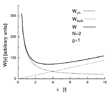
Figure 2: Energy of the saddle-point solution.

A.1.2 The energy of the chiral edges.

As we already pointed out, the discontinuities of the function $\gamma(\varphi)$ determine a set of one-dimensional curves (“strings”) where the chiral degrees of freedom reside. At the level of the saddle-point solution these are static straight lines at $y=n\lambda$ and $y=(n+\nu)\lambda$, with $n$ integer.

Upon integrating over the array of chiral bosons, and taking into account that $\varphi$ is static, we can calculate the contribution of the edges to the energy per period. Since the saddle-point solution $\varphi$ is independent of $x$, and $\varphi(0)=\varphi(\nu\lambda)$ and $\partial_{y}\varphi(0)=-\partial_{y}\varphi(\nu\lambda)$, we find that the energy per period per unit length (along the $x$ axis) is

$$\tilde{W}_{\rm edge}=\frac{\varphi(0)^{2}}{\left|\partial_{y}\varphi(0)\right|}$$ (66)

In terms of the explicit solution Eq. 56, Eq. LABEL:phiN, and Eq. LABEL:phiN+1, this energy reads

$$\tilde{W}_{\rm edge} = \frac{g\omega_{c}}{\xi_{N+1}}\frac{\sinh\left(\frac{\lambda}{2}[\xi_{N}\nu+\xi_{N+1}(1-\nu)]\right)}{\sinh\left(\frac{\lambda}{2}\xi_{N+1}[1-\nu]\right)\sinh\left(\frac{\lambda}{2}\xi_{N}\nu\right)}$$

$$\times\left[N+\right. \left.\frac{\xi_{N+1}}{\xi_{N}}\frac{\sinh\left(\frac{\lambda}{2}\xi_{N+1}[1-\nu]\right)\cosh\left(\frac{\lambda}{2}\xi_{N}\nu\right)}{\sinh\left(\frac{\lambda}{2}[\xi_{N}\nu+\xi_{N+1}(1-\nu)]\right)}\right]^{2}$$

For large $\lambda$ this function approximates exponentially fast a constant, and it diverges like $1/\lambda$ for small values of the period.

Thus, the total energy per period of the saddle-point solution is

$$\tilde{W}=\tilde{W}_{\rm bulk}+\tilde{W}_{\rm edge}$$ (68)

where $\tilde{W}_{\rm bulk}$ and $\tilde{W}_{\rm edge}$ are given by Eq. 63 and Eq. LABEL:edgeenergy respectively. In figure 2 we depict these functions. We see that the competition between bulk and edge energies yields a stable and finite value of the period $\bar{\lambda}$.

A.2 The $N\gg 1$ limit

In order to clarify the dependence of the optimal period $\bar{\lambda}$ with the microscopic parameters of the theory it is convenient to consider particular limits where the expressions for the energy become tractable. In particular, it is possible to find an explicit analytic result for the period of the stripe in the limit $N\gg 1$ (c. f. ref. chalker ). In this limit, $\xi_{N}/\xi_{N+1}=1+{\cal O}(1/N)$, and the energy $\tilde{W}$ given by Eq. 68 becomes

$$\tilde{W}=g\omega_{c}\frac{N^{2}}{\xi_{N}} \!\!\!\!\!\!\left\{\left(\frac{1+g}{g}\right)\frac{\lambda\xi_{N}}{2}\right.$$ (69)

$$+ \left.\frac{\sinh\left(\frac{\lambda}{2}\xi_{N}\right)}{\sinh\left(\frac{\lambda}{2}\xi_{N}[1-\nu]\right)\sinh\left(\frac{\lambda}{2}\xi_{N}\nu\right)}\right\}$$

Note that $\lambda$ always appears in the combination $\lambda\xi_{N}/2$. This means that the natural scale for the period is $\xi_{N}/2$. In terms of the variable $\bar{x}=\frac{\lambda\xi_{N}}{2}$, the extremal condition

$$\frac{d\tilde{W}(\bar{x})}{d\bar{x}}=0$$ (70)

becomes

$$\nu\;{\rm csech}^{2}(\nu\bar{x})+(1-\nu)\;{\rm csech}^{2}((1-\nu)\bar{x})=\frac{g+1}{g}$$ (71)

For $\nu=1/2$ we find the explicit solution

$$\bar{x}=2\sinh^{-1}\left\{\sqrt{\frac{g}{g+1}}\right\}$$ (72)

Thus, the period of the stripe, for large $N$ and $\nu=1/2$, is

$$\bar{\lambda}=4\sqrt{gN+a^{2}}\sinh^{-1}\left\{\sqrt{\frac{g}{g+1}}\right\}\;\ell$$ (73)

Eq. 73 implies that the period of the stripe is set by a combination of the cyclotron radius of the partially filled Landau level ${\sqrt{N}}\ell$, the range of the interaction $a$, and a function of the dimensionless coupling constant $g$. In particular, the wavelength of the stripe state is of the order of the cyclotron radius only in the limit in which the dimensionless range of the interaction is small, $a\ll{\sqrt{gN}}$. In this limit, the result of Eq. 73 agrees with the estimates of Koulakov and coworkersfogler . It turns out that expression Eq. 73 is a very good approximation even for small values of $N$. In fig. 3 we compare the numerical solution of the period for $N=4$ with the large $N$ approximation. Notice that the position of the optimal value of $\lambda$ is essentially the same for both curves.

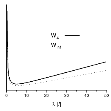
Figure 3: Comparison between the energy for $N=4$ and the $N\to\infty$ limit

We can also solve equation (71) when $\nu\approx 1$. In this case the period of the stripe is written as

$$\bar{\lambda}=\left(\frac{2}{1-\nu}\right)\sqrt{\frac{g}{g+1}}\sqrt{gN+a^{2}}\ell$$ (74)

It turns out that the period increases as the filling factor increases (away from $1/2$). In any case, we expect that for filling factors not too close to $1/2$ the stripe state should become unstable to other types of phases, such as a bubble phasefogler , a stripe crystalFK ; MF ; fertig and possibly a quantum nematic phaseFK ; FKMN .

Appendix B The geometrical couplings

In this section we derive the effective action for the chiral edge states of the stripe state. Qualitatively this problem is very much analogous to that of the fermion zero modes bound to a dynamical domain wallfosco . Here we will show how a geometrical electric field is induced on the stripe due to its dynamics.

The action for two-dimensional fermions in a magnetic field and a time dependent background potential $\varphi$ is

$$S=\int d^{3}z~{}\left[\psi^{*}(z)[iD_{0}-\mu-e\varphi]\psi(z)+\frac{1}{2m}\left|{\bf D}\psi(z)\right|^{2}\right]$$ (75)

where ${\bf D}_{i}=\partial_{i}+iA_{i}$ and $\vec{\nabla}\times{\vec{A}}=B{\hat{z}}$.

The Hubbard-Stratonovich field $\varphi$ behaves like a scalar potential in electrodynamics. As such it (adiabatically) deforms of the Landau levels. If the topmost filled Landau level $N$ crosses the chemical potential at some set of smooth curves,

$$\varphi\left(\bar{x}(s,t),\bar{y}(s,t),t\right)=E_{N}-\mu$$ (76)

then the system has gapless excitations with support on these curves, which thus behave as dynamical edges. Here $E_{N}$ is the energy of the $N^{\rm th}$ Landau level. This equation defines a time dependent string-like object, a two-dimensional surface embedded in a Euclidean three dimensional space-time, whose position is defined by $\vec{R}(s,t)=(\bar{x}(s,t),\bar{y}(s,t))$. For the most part it will be sufficient to consider only one edge at a time.

Let us expand the potential $\varphi$ around its constant value on the string

$$\varphi(x,y,t)=\varphi(\bar{x},\bar{y},t)+\tilde{v}\hat{n}_{\mu}x_{\mu}$$ (77)

where

$$\tilde{v}=\left|\partial_{\mu}\varphi\right|=\sqrt{\left(\frac{\partial\varphi}{\partial t}\right)^{2}+\left|\vec{\nabla}\varphi\right|^{2}}$$ (78)

and $n_{\mu}$ is a unit vector perpendicular to the surface defined by Eq. 76. The effective action in this approximation is

$$S=\int d^{3}z~{}\left[\psi^{*}\left(iD_{0}-E_{N}+\tilde{v}\hat{n}_{\mu}x_{\mu}\right)\psi+\frac{1}{2m}\left|{\bf D}\psi\right|^{2}\right]$$ (79)

To proceed with the calculation, we rewrite the action in generalized coordinates

$$x_{\mu}=(x_{0},x_{1},x_{2})\rightarrow\xi_{\mu}=(\xi_{0},\xi_{1},\xi_{2})$$

The coordinate transformation and the metric is defined by $\xi_{\mu}=\frac{\partial\xi_{\mu}}{\partial x_{\nu}}~{}x_{\nu}$ and $g_{\mu\nu}=\frac{\partial x^{\alpha}}{\partial\xi^{\mu}}\frac{\partial x^{\beta}}{\partial\xi^{\nu}}\delta_{\alpha\beta}$ respectively. It is convenient to choose a coordinate system defined by

$$\xi_{2}=\hat{n}_{\mu}x_{\mu}$$ (80)

in such a way that the differential quadratic form is given by

$$ds^{2}=d\xi_{2}^{2}+g_{ab}d\xi^{a}d\xi^{b}~{}~{}~{}~{}{\rm where}~{}~{}~{}~{}a,b=0,1$$ (81)

In these coordinates the domain wall is defined by the equation $\xi_{2}=0$ and the action of Eq. 79 now reads

$$S = \int d^{3}\xi~{}\sqrt{g}\left[\psi^{*}(\xi)[i\left(\frac{\partial\xi_{\mu}}{\partial t}\right)\frac{\partial~{}}{\partial\xi_{\mu}}+\tilde{v}\xi_{2}-E_{N}]\psi(z)\right.$$ (82)

$$+ \left.\frac{1}{2m}\eta^{\mu\nu}\left|{\bf D}\psi(\xi)\right|^{2}\right]$$

where we have used the notation

$$\eta_{\mu\nu}=\frac{\partial\xi_{\mu}}{\partial x_{i}}\frac{\partial\xi_{\nu}}{\partial x_{i}}\;,\qquad g=|{\rm det}g_{\mu\nu}|$$ (83)

It is now convenient to choose the Landau gauge in the new coordinates

$$A_{0}=0\mbox{~{}~{}~{}~{},~{}~{}~{}~{}}A_{1}=B\xi_{2}\mbox{~{}~{}~{}~{},~{}~{}~{}~{}}A_{2}=0$$ (84)

Next we expand the Fermi field $\psi$ in the new coordinates and find

$$\psi(\xi_{0},\xi_{1},\xi_{2})=\sum_{n,p}C_{n,p}X^{n}(\xi_{1})Y^{n}_{p}(\xi_{2})T^{n}(\xi_{0})$$ (85)

The set of functions $\{X^{n}(\xi_{1}),Y^{n}_{p}(\xi_{2}),T^{n}(\xi_{0})\}$ constitute complete basis, and satisfy the eigenvalue equations

$$i\partial_{0}T^{n} = \omega_{n}T^{n}$$ (86)

$$i\partial_{1}X^{n} = k_{n}X^{n}$$ (87)

$$\left\{-\frac{\eta^{\mu 2}\eta^{\mu 2}}{2m}\partial_{2}^{2}-2B\eta^{\mu 1}\eta^{\mu 2}\left(\xi_{2}-\frac{m\tilde{v}}{(\eta^{\mu 1})^{2}}B^{2}\right)\partial_{2}\right.$$ (88)

$$+ \left.\frac{(\eta^{\mu 1})^{2}}{2m}\xi_{2}^{2}-E_{N}\right\}Y^{n}_{p}=\lambda_{n,p}Y^{n}_{p}$$

Eq. 88 is nothing but the eigenvalue equation for the linear harmonic oscillator (in generalized coordinates). By inspection we see that Eq. 88 has a zero mode $\lambda_{n,P}=0$ provided $E_{N}$ is the energy of a Landau level in the undistorted coordinates. Upon substitution Eq. 85 into Eq. 79, using the usual orthogonality relations for the oscillator eigenfunctions, and after factoring out the zero mode from the rest of the spectrum, we find that the effective action for the zero mode is given by

$$S_{0}=\int d^{2}\xi~{}\sqrt{g}~{}\frac{1}{2}\left\{\psi_{0}^{*}(\xi){\cal D}\psi_{0}(\xi)-{\cal D}\psi_{0}^{*}(\xi)\psi_{0}(\xi)\right\}$$ (89)

where

$${\cal D}=\left(\frac{\partial\xi_{0}}{\partial t}-v\eta^{\mu 1}\eta^{\mu 0}\right)\frac{\partial~{}}{\partial\xi_{0}}-\left(v\eta^{\mu 1}\eta^{\mu 1}-\frac{\partial\xi_{1}}{\partial t}\right)\frac{\partial~{}}{\partial\xi_{1}}$$ (90)

Here we have defined $v\equiv{\tilde{v}}/B$.

For the problem of interest here, we will specialize these results to the case of a stripe whose mean position is a straight line along the $x$ axis, as defined in the saddle-point approximation of section III. To this aim in mind, we define a coordinate system as follows

$$x_{0} = \xi_{0}$$

$$x_{1} = \xi_{1}$$

$$x_{2} = \delta(\xi_{0},\xi_{1})\equiv\frac{\delta\varphi(\xi_{0},\xi_{1},x_{2}=0)}{\left|\partial_{x_{2}}\varphi(x_{2}=0)\right|}$$ (91)

where $\delta(\xi_{0},\xi_{1})$ is an infinitesimal local displacement of the position of the edge. In this coordinate system the effective action can be cast in the form

$$S=\int d^{2}\xi~{}\sqrt{g}~{}\left\{\psi_{0}^{*}(\xi)\left(\partial_{0}-v\partial_{1}\right)\psi_{0}(\xi)+\Gamma\psi_{0}^{*}(\xi)\psi_{0}(\xi)\right\}$$ (92)

where $\Gamma=\frac{1}{2}g^{-\frac{1}{2}}{\cal D}g^{\frac{1}{2}}$. This quantity couples in the same way that a gauge field couples to a chiral zero mode. Notice that this gauge field looks like a pure gauge and as such it would seem that it should have no effect on the theory. That would be indeed the case if the theory of the zero modes was gauge invariant all on its own right. However, this is not the case here as these modes have a gauge anomaly.

Eq. 92 is precisely the action of a one dimensional chiral fermion in curved spacetime. It is very well known that this system is anomalous and as a consequence the divergence of the current is proportional to the curvature of the space-time. As a matter of fact, the current $J$ of the chiral fermion satisfies,

$$\partial_{0}J_{0}+v\partial_{1}J_{1}={\rm det}\left(\frac{\partial^{2}\delta(\xi_{0},\xi_{1})}{\partial_{\xi_{a}}\partial_{\xi_{b}}}\right)$$ (93)

to leading order in $\delta(\xi_{0},\xi_{1})$. Therefore, within this approximation, Eq. 93 reduces to the divergence of the edge current in Cartesian coordinates. Hence, we are led to interpret the quantity ${\rm det}\left(\frac{\partial^{2}\delta(\xi_{0},\xi_{1})}{\partial_{\xi_{a}}\partial_{\xi_{b}}}\right)$ as an induced geometrical electric field given by

$$E_{\rm geom}=\frac{1}{v}\partial^{2}_{1}\delta\partial_{0}^{2}\delta-(\partial_{0}\partial_{1}\delta)^{2}$$ (94)

The same expression for the geometrical electric field was also derived for a system of Dirac fermions with time-dependent domain wallsfosco . It is straightforward to see that $E_{\rm geom}$ is generated by the “dynamical electromagnetic potential”

$$A^{\rm dyn}_{0} = \partial_{1}\delta\partial^{2}_{0}\delta$$ (95)

$$A^{\rm dyn}_{1} = \partial_{1}\delta\partial_{1}\partial_{0}\delta$$ (96)

We have used this type of couplings on the second line of Eq. 22.

Appendix C Charge conservation, cancelation of anomalies and the Callan-Harvey effect.

In this Appendix we show that charge conservation in a stripe state is realized thorough an anomaly cancelation mechanism that includes the effects of dynamical edges.

The problem that needs to be addressed here is that we have separated the dynamical degrees of freedom into a “bulk” piece , given by Eq. 17 and Eq. 16, and an “edge” piece, Eq. 20. It turns out that the $U(1)$ gauge transformation of the external gauge field is not a symmetry of each part of this action separately, but instead it is a symmetry of the full system. this problem is quite familiar in the physics of the QHEwen ; frohlich ; Haldane ; Kao . The main difference in the problem of interest here is that the edges are not static. This subtle cancelation of anomalies is an example of the well known Callan-Harvey mechanismCH .

To illustrate the point, let us consider a general time dependent gauge transformation,

$${\tilde{A}}_{0}\rightarrow{\tilde{A}}_{0}+\partial_{0}\alpha(x,y,t)~{}~{}~{}~{}~{}~{}~{}~{}~{}~{}~{}{\tilde{A}}_{i}\rightarrow{\tilde{A}}_{i}+\partial_{i}\alpha(x,y,t)$$ (97)

The only term in the bulk action that it is not gauge invariant is the Chern-Simons term for the electromagnetic perturbations

$$W_{\rm C-S}=\frac{e^{2}}{4\pi}\int d^{3}x~{}\gamma(\varphi)\epsilon_{\mu\nu\rho}{\tilde{A}}_{\mu}\partial_{\nu}{\tilde{A}}_{\rho}$$ (98)

where $\gamma(\varphi)=\sum_{n=0}^{\infty}\Theta\left(\mu-E_{n}+\varphi\right)$ and $E_{n}=(n+\frac{1}{2})\omega_{c}$, where $\Theta(x)$ is the step function. All the other terms in $S_{\rm eff}$ are gauge invariant.

The variation of the Chern-Simons action Eq. 98 is,

$$\delta W_{\rm C-S}=-\frac{e^{2}}{4\pi}\int d^{3}x \left\{\partial_{\mu}\gamma(\varphi)\epsilon_{\mu\nu\rho}\partial_{\nu}{\tilde{A}}_{\rho}-\right.$$ (99)

$$\left.\partial_{\mu}\left(\alpha\epsilon_{\mu\nu\rho}\partial_{\nu}{\tilde{A}}_{\rho}\right)\right\}$$

which can be split in two terms

$$\delta W_{C-S}=\delta_{\cal E}W+\delta_{\cal B}W$$ (100)

with

$$\delta_{\cal E}W = \frac{e^{2}}{2\pi}\int d^{3}x~{}\left[-\alpha\partial_{i}\gamma(\varphi)\epsilon_{ij}{\cal E}_{j}+\partial_{i}\left\{\alpha\gamma(\varphi)\epsilon_{ij}{\cal E}_{j}\right\}\right]$$

$$\delta_{\cal B}W = \frac{e^{2}}{2\pi}\int d^{3}x~{}\left[-\alpha\partial_{0}\gamma(\varphi){\cal B}+\partial_{0}\left\{\alpha\gamma(\varphi){\cal B}_{j}\right\}\right]$$

where ${\cal E}_{j}=\partial_{i}{\tilde{A}}_{0}-\partial_{0}{\tilde{A}}_{i}$ and ${\cal B}=\epsilon_{i,j}\partial_{i}{\tilde{A}}_{j}$ are the electric and magnetic field associated to ${\tilde{A}}_{\mu}$. If $\gamma(\varphi)$ is a constant, then $\delta W=0$ up to boundary terms. However,

$$\partial_{\mu}\gamma(\varphi)=\sum_{n}\delta\left(\mu-E_{n}+\varphi\right)\partial_{\mu}\varphi$$ (103)

Thus, in the presence of an electromagnetic field, and for $N$ completely filled Landau Levels, we have

$$\delta_{\cal E}W = -\frac{e^{2}}{2\pi}\int d^{3}x\;\alpha\;\delta\left(\mu-E_{N}+\varphi\right)\epsilon_{ij}\partial_{j}\varphi{\cal E}_{i}$$ (104)

$$+ \frac{e^{2}}{2\pi}\int d^{3}x~{}\partial_{i}\left\{\alpha\gamma(\varphi)\epsilon_{ij}{\cal E}_{j}\right\}$$

$$\delta_{\cal B}W = -\frac{e^{2}}{2\pi}\int d^{3}x\;\alpha\;\delta\left(\mu-E_{N}+\varphi\right)\partial_{t}\varphi{\cal B}$$ (105)

$$+ \frac{e^{2}}{2\pi}\int d^{3}x~{}\partial_{0}\left\{\alpha\gamma(\varphi){\cal B}_{j}\right\}$$

The first integral of (104) has support on a one dimensional dynamical string $\partial\Omega$ defined by

$$\partial\Omega:\left\{\varphi(x,y,t)=E_{N}-\mu\right\}$$ (106)

The second integral is a surface term, on a surface that contains the string, Eq. 106. Explicitly we find

$$\delta_{\cal E}W=\pm\frac{e^{2}}{\pi}\int_{R\times\partial\Omega}dsdt~{}\alpha~{}~{}\hat{t}\cdot\vec{\cal E}(s,t)$$ (107)

where $\hat{t}_{i}=\epsilon_{ij}\partial_{j}\varphi/|\vec{\nabla}\varphi|$ is a unit vector tangent to the strings $\partial\Omega$. The $\pm$ sign is the orientation of the curve.

$\delta_{\cal B}W$, of Eq.  105, does not vanish because $\varphi$ is in general a time-dependent function. Then, by using Eq. 24 it is possible to write $\delta_{\cal B}W$ as a function of the variation of the actual position of the string in the form

$$\delta_{\cal B}W=\pm\frac{e^{2}}{\pi}\int_{R\times\partial\Omega}dsdt~{}\alpha~{}~{}\left(\frac{\partial\vec{R}}{\partial t}\cdot\hat{n}\right)~{}{\cal B}(s,t)$$ (108)

From Eq. 107 and Eq. 108 we see that the divergence of the current in the bulk is

$$\partial_{t}\rho+\partial_{i}J_{i}=\pm\frac{e^{2}}{\pi}\left\{\hat{t}\cdot\vec{\cal E}+\left(\frac{\partial\vec{R}}{\partial t}\cdot\hat{n}\right)~{}{\cal B}\right\}$$ (109)

where the ${\cal E}$ and ${\cal B}$ have support on the strings $\partial\Omega$ defined in Eq. 106.

It is not difficult to show that this divergence is canceled against the divergence of the currents of the chiral edge states derived in Eq. 20. The induced current at the edge

$$J_{s}=\mp\frac{e^{2}}{\pi}\frac{\partial_{s}^{2}}{\partial_{0}\partial_{s}\mp v\partial_{s}^{2}}\left\{{\tilde{A}}_{0}(s,t)+\left(\frac{\partial\vec{R}}{\partial t}\cdot\hat{n}\right)~{}{\tilde{A}}_{n}(s,t)\right\}$$

Here we have assumed the gauge ${\tilde{A}}_{i}{\hat{t}}_{i}=0$, where ${\tilde{A}}_{n}$ is the component of the vector potential locally normal to the strings. Evaluating the divergence of this current, we find

$$\left(\partial_{0}\mp v\partial_{s}\right)J_{s} = \mp\frac{e^{2}}{\pi}\left\{\partial_{s}{\tilde{A}}_{0}+\left(\frac{\partial\vec{R}}{\partial t}\cdot\hat{n}\right)~{}\partial_{s}{\tilde{A}}_{n}\right\}$$

$$= \mp\frac{e^{2}}{\pi}\left\{\hat{t}\cdot\vec{\cal E}+\left(\frac{\partial\vec{R}}{\partial t}\cdot\hat{n}\right)~{}{\cal B}(s,t)\right\}$$

which cancels exactly Eq. 109. In Eq. LABEL:divedge we ignored terms proportional to $\partial_{s}\left(\frac{\partial\vec{R}}{\partial t}\cdot\hat{n}\right)$ since they can be absorbed in a reparametrization of the curve $s\to f(s,t)$.

Appendix D Fluctuation propagators

The propagators ${\cal F}^{\alpha\beta}$ of Eq. 38 are the inverse of the fluctuation operator

$$\left.\frac{\delta^{2}S_{\varphi}}{\delta\varphi(x^{\prime})\delta\varphi(x)}\right|=-\left\{\left(\gamma(\varphi)+{\frac{a^{2}}{g}}\right)\nabla^{2}-\frac{1}{g}\right\}\delta(x-x^{\prime})$$

(112)

without the zero modes. In other words we need to evaluate the Green function

$$\left\{\left(\gamma(\varphi(x))+{\frac{a^{2}}{g}}\right)\nabla^{2}-\frac{1}{g}\right\}G(\vec{x},\vec{x}^{\prime})=-2\pi\delta(\vec{x}-\vec{x}^{\prime})$$

(113)

subject to the condition that $G(\vec{x},\vec{x}^{\prime})=0$ when $|\vec{x}-\vec{x}^{\prime}|\to\infty$. These boundary conditions automatically take off the zero modes since exclude any fluctuation that could globally translate or rotate the system. Notice that this propagator is static, i. e. it is instantaneous. This feature is a consequence of the local incompressibility of the bulk regions. Eq. 113 is a singular partial differential equation due to the presence of the function $\gamma(\varphi(x))$. Defining the function $f(y)$ as

$$f(y)=\left\{\begin{array}[]{lcc}N+\frac{a^{2}}{g}&&n\lambda\leq y<(N+\nu)\lambda\\ N+1+\frac{a^{2}}{g}&&(n+\nu)\lambda\leq y<(n+1)\lambda\end{array}\right.$$ (114)

with $n$ integer and $0<\nu<1$, considering also a smooth regularization of $f(y)$ (i. e. finite temperature) and Fourier transforming in the coordinate $x$

$$G(x-x^{\prime};y,y^{\prime})=\int\frac{dq_{x}}{2\pi}e^{iq_{x}(x-x^{\prime})}G(q_{x};y,y^{\prime})$$ (115)

we arrive to the following differential equation in $y$

$$\left[-f(y)\frac{d^{2}~{}}{dy^{2}}+\left(q_{x}^{2}f(y)+\frac{1}{g}\right)\right]G(q_{x};y,y^{\prime})=$$

$$(2\pi)^{2}\delta(y-y^{\prime})$$ (116)

with

$$G(q_{x};y+\lambda,y^{\prime}+\lambda)=G(q_{x};y,y^{\prime})$$ (117)

To solve Eq. 116 we adopt a recursive method. First we solve the equation for an arbitrary period $n$ (away form the position of the function $\delta$). In this case we have

$$\left[-f(y)\frac{d^{2}~{}}{dy^{2}}+\left(q_{x}^{2}f(y)+\frac{1}{g}\right)\right]F_{n}(y)=0$$ (118)

A general solution reads,

$$F^{-}_{n}(y)=A_{n}^{-}e^{K_{-}(y-n\lambda)}+B^{-}_{n}e^{-K_{-}(y-n\lambda)}$$ (119)

for $n\lambda\leq y<(n+\nu)\lambda$ and

$$F^{+}_{n}(y)=A_{n}^{+}e^{K_{+}(y-(n+\nu)\lambda)}+B^{+}_{n}e^{-K_{+}(y-(n+\nu)\lambda)}$$ (120)

for $(n+\nu)\lambda\leq y<(n+1)\lambda$, where we defined

$$K_{-}^{2} = q_{x}^{2}+\frac{1}{gN+a^{2}}$$ (121)

$$K_{+}^{2} = q_{x}^{2}+\frac{1}{g(N+1)+a^{2}}$$ (122)

Imposing the continuity of the function $F_{n}(y)$ and its derivative $F^{\prime}_{n}(y)$ at the points $y=(n+\nu)\lambda$ and $y=(n+1)\lambda$ it is possible to find a relation between the coefficients of the solution in different periods. In matrix notation this relation reads

$$\left(\begin{array}[]{c}A_{n}^{-}\\ B_{n}^{-}\end{array}\right)=M^{n}\left(\begin{array}[]{c}A_{0}^{-}\\ B_{0}^{-}\end{array}\right)$$ (123)

and

$$\left(\begin{array}[]{c}A_{n}^{+}\\ B_{n}^{+}\end{array}\right)=(M^{\prime})^{n}\left(\begin{array}[]{c}A_{0}^{+}\\ B_{0}^{+}\end{array}\right)$$ (124)

where $M$ and $M^{\prime}$ are two $2\times 2$ matrices (functions of $K_{+}$ and $K_{-}$) with unit determinant and the subindex $0$ indicates and arbitrary fixed period chosen as the origin of coordinates. Similar equations, involving the inverse matrices $M^{-1}$ and $M^{\prime-1}$ can be found for negative values of $n$.

The propagators we are looking for are given by

$${\cal F}^{++}_{n} = F^{-}_{n}(n\lambda)=A_{n}^{-}+B_{n}^{-}$$ (125)

$${\cal F}^{+-}_{n} = F^{+}_{n}((n+\nu)\lambda)=A_{n}^{+}+B_{n}^{+}$$ (126)

Therefore, in order to guarantee the boundary condition

$$\lim_{n\to\pm\infty}{\cal F}^{\alpha\beta}_{n}=0$$ (127)

we choose $(A_{0}^{-},B_{0}^{-})$ to be an eigenvector of $M$ with eigenvalue $m_{-}<1$. For concreteness let us define the vector $(\alpha_{-},\beta_{-})$ such that

$$M\left(\begin{array}[]{c}\alpha_{-}\\ \beta_{-}\end{array}\right)=m_{-}\left(\begin{array}[]{c}\alpha_{-}\\ \beta_{-}\end{array}\right)$$ (128)

with $m_{-}<1$ and $\alpha_{-}^{2}+\beta_{-}^{2}=1$. In this way we can write

$$\left(\begin{array}[]{c}A_{n}^{-}\\ B_{n}^{-}\end{array}\right)=a\;m_{-}^{n}\left(\begin{array}[]{c}\alpha_{-}\\ \beta_{-}^{-}\end{array}\right)$$ (129)

where $a$ is an arbitrary coefficient. We can write a similar expression for negative $n$

$$\left(\begin{array}[]{c}A_{-n}^{-}\\ B_{-n}^{-}\end{array}\right)=b\;m_{-}^{n-1}\left(\begin{array}[]{c}\alpha_{+}\\ \beta_{+}\end{array}\right)$$ (130)

where $(\alpha_{+},\beta_{+})$ is a unit eigenvector of the matrix $M^{-1}$. (the eigenvalue is the same due to ${\rm det}M=1$).

Finally, let us suppose that the $\delta$-function has support in $y^{\prime}=0$. We can determine the two unknown coefficients $a$ and $b$ by asking continuity of the function and discontinuity of the derivative at the origin.

$$F_{0}^{-}(0)-F_{-1}^{+}(0) = 0$$ (131)

$$\left.\frac{dF_{0}^{-}}{dy}\right|_{y=0}-\left.\frac{dF_{-1}^{+}}{dy}\right|_{y=0} = -\frac{(2\pi)^{2}}{f(0)}$$ (132)

where we choose the regularization of $f(y)$ such that $f(0)=N+\frac{a^{2}}{g}+\frac{1}{2}$.

Following this tedious by direct algebra it is possible to exactly determine the propagators of Eq. 125 and Eq. 126. Although the result is a complicated expression, it can be cast in a simpler form considering the limit $Ng+a^{2}>>g$ and $\nu=1/2$. In this limit, the difference $\delta=K_{+}-K_{-}$ is an infinitesimal quantity and the propagators to leading order in $\delta$ read

$${\cal F}^{++}_{n}(q_{x})=2\pi^{2}\frac{e^{-|n|K_{-}\lambda}}{K_{-}(N+\frac{a^{2}}{g})}$$ (133)

$${\cal F}^{+-}_{n}(q_{x})=2\pi^{2}\frac{e^{-K_{-}\lambda/2}}{K_{-}(N+\frac{a^{2}}{g})}\left\{\begin{array}[]{lcl}e^{-nK_{-}\lambda}&&n\geq 0\\ &&\\ e^{(n+1)K_{-}\lambda}&&n<0\end{array}\right.$$ (137)

(138)

To obtain the propagators in momentum $q_{y}$ space we make the following Fourier transformation

$${\cal F}^{\alpha\beta}(q_{x},q_{y})=\sum_{n=-\infty}^{\infty}{\cal F}_{n}^{\alpha\beta}(q_{x})e^{iq_{y}n}$$ (139)

It is straightforward to obtain

$${\cal F}^{++} = 16\pi^{2}\;v\;\frac{\sinh(K_{-}\lambda)}{K_{-}\lambda}\frac{1}{\cosh(K_{-}\lambda)-\cos q_{y}}$$

$${\cal F}^{+-} = 16\pi^{2}\;v\;\frac{\sinh(K_{-}\lambda/2)}{K_{-}}\frac{(1+e^{-iq_{y}})}{\cosh(K_{-}\lambda)-\cos q_{y}}$$

where in this approximation

$$v=\frac{1}{2}\frac{g^{3/2}}{\sqrt{gN+a^{2}}}$$ (142)

In the long wavelength limit, $q_{x}\to 0$ and $q_{y}\to 0$, the kernels ${\cal F}_{\alpha\beta}(q)$ take the finite limiting values

$${\cal F}^{++}(0) = \frac{16\pi^{2}{v}}{\lambda\xi_{N}}\coth\left(\lambda\xi_{N}/2\right)$$ (143)

$${\cal F}^{+-}(0) = \frac{16\pi^{2}{v}}{\lambda\xi_{N}}\frac{1}{\sinh\left(\lambda\xi_{N}/2\right)}$$ (144)

which are simple smooth functions of the coupling constant.

Appendix E Elastic constants

In this appendix we show some details of the calculation of the constants $Q$, $\kappa_{\perp}$ and $\kappa_{\parallel}$ that enter the action of Eq. LABEL:Susmectic.

The elastic constants $Q$ and $\kappa_{\perp}$ are obtained by replacing in $S_{\varphi}$ (Eq. 16) the deformed saddle-point solution $\varphi(u)$ (Eq. 32). The main contribution to $Q$ comes from the first term of Eq.  16,

$$\int\frac{d^{3}x}{4\pi}\;\frac{3\gamma^{2}}{8}(\partial^{2}_{x}\varphi(u))^{2}=\int\frac{d^{3}x}{4\pi}\;\frac{3\gamma^{2}(\varphi^{\prime})^{2}}{8}(\partial^{2}_{x}u)^{2}$$ (146)

where $\varphi^{\prime}$ is the derivative of $\phi$. While the term $\partial^{2}_{x}u$ in Eq. 146 is a slowly varying function of $y$ in a scale long with respect to the stripe period $\lambda$, the expression $\gamma^{2}(\varphi^{\prime})^{2}$ is a rapidly varying function within a period $\lambda$. Therefore, at long distances, we can safely take the mean value of the last expression over one period, obtaining

$$\int\frac{d^{3}x}{4\pi}\;\frac{3\gamma^{2}}{8}(\partial^{2}_{x}\varphi(u))^{2}=\int d^{3}x\;Q\;\;(\partial^{2}_{x}u)^{2}$$ (147)

where we have defined

$$Q=\frac{3}{32\pi\lambda}\int_{0}^{\lambda}dy~{}\left(\gamma(\varphi)\frac{\partial\varphi(y)}{\partial y}\right)^{2}$$ (148)

In momentum space, this corse-graining procedure is equivalent to take the zero momentum limit of the Fourier transform of $\gamma(\varphi)\phi^{\prime}$. We simply obtain

$$Q=\frac{3}{32\pi}N^{2}v^{2}$$ (149)

In the limit $Ng+a^{2}>>g$ we can use Eq.142 for the velocity obtaining

$$Q=\frac{3}{128\pi}\;\frac{N^{2}g^{2}}{gN+a^{2}}$$ (150)

In Eq. 49 we show the value of $Q$ for a very short ranged potential $a\to 0$.

The compressibility $\kappa_{\perp}$ is nothing but the energy density per period of the saddle-point configuration calculated in Appendix A (see Eq.  69). To formally obtain this expression we proceed as follows: first we substitute $\varphi$ by the deformed saddle-point $\varphi(u)$ in Eq. 16. Then we performed the change of variables $y^{\prime}=y\alpha+u$ obtaining to leading order in the derivatives of $u$

$$\int d^{3}x{\cal L}(\varphi(u(x,y)))\approx\int d^{3}x{\cal L}(\varphi(y))$$

$$+ \frac{1}{2}\int d^{3}x{\cal L}(\varphi(y))\left(\frac{\partial u}{\partial y}\right)^{2}+\ldots$$

Again, in the last integral, the factor ${\cal L}(\varphi)$ is a periodic function of $y$ with period $\lambda$, while $\partial_{y}u$ is a slowly varying function of $y$. Therefore we can take the mean value of ${\cal L}(\varphi)$ on a period defining in this way

$$\kappa_{\perp} = \frac{1}{2\lambda}\int_{0}^{\lambda}dy~{}\left\{\left[\gamma+\frac{a^{2}}{2g}\right]\left(\frac{\partial\varphi(y)}{\partial y}\right)^{2}+\gamma\varphi\right.$$ (152)

$$+ \left.\left(\frac{1}{2g}+\frac{v+{\cal F}^{++}-{\cal R}e{\cal F}^{+-}}{(v+{\cal F}^{++})^{2}-|{\cal F}^{+-}|^{2}}\right)\varphi^{2}\right\}$$

where $\varphi$ is the undeformed saddle-point solution. The kernels ${\cal F}^{++}$ and ${\cal F}^{+-}$ come from the contribution of the chiral modes to the action and are given in Appendix IV. Notice that only the ${\vec{q}}\to 0$ limit of this kernels is important here. In the limit $gN+a^{2}>>g$ and $g<<1$ this expression is given by,

$$\kappa_{\perp}=\frac{5}{4}N^{2}g^{1/2}\sqrt{gN+a^{2}}$$ (153)

The dynamical term in Eq. LABEL:Susmectic comes form the Gaussian integral of the chiral modes and is given by Eq. 44. We can rewrite it more explicitly as

$$-\frac{1}{2}\sum_{nm}\int d^{2}xd^{2}x^{\prime}\;\varphi^{\prime}_{n}\varphi^{\prime}_{m}\;\Pi_{mn}\;\partial_{x}u_{m}\partial_{x}u_{n}$$ (154)

where

$$\Pi_{mn}=\left\{\pi_{++}^{-1}+\pi_{--}^{-1}-\pi_{+-}^{-1}-\pi_{-+}^{-1}\right\}_{mn}$$ (155)

Calculating the inverse matrix $\pi^{-1}$, subtracting the static part, and taking the continuum limit as in the preceding cases we finally find the dynamical contribution to the Lagrangian (in momentum space),

$${\cal L}_{\rm dyn}=-\frac{1}{2}K\frac{\omega^{2}}{\omega^{2}-\bar{v}^{2}q_{x}^{2}}$$ (156)

where the renormalized velocity is given by

$$\bar{v}^{2}=(v+{\cal F}^{++})^{2}-|{\cal F}^{+-}|^{2}$$ (157)

and the constant $K$ can be calculated from

$$K=\frac{1}{\lambda}\int_{0}^{\lambda}dy\frac{v+{\cal F}^{++}-{\cal R}e{\cal F}^{+-}}{((v+{\cal F^{++}})^{2}-|{\cal F}^{+-}|^{2})}\left(\frac{\partial\varphi}{\partial y}\right)^{2}$$ (158)

From Eq. 44 we have that

$$\kappa_{\parallel}=\frac{\bar{v}^{2}}{K\lambda}$$ (159)

Using the expression for ${\cal F}^{\alpha\beta}$ given in Appendix D we find in the limit $Ng+a^{2}>>1$ and $g<<1$

$$\kappa_{\parallel}=\frac{\pi^{2}}{16}\;g^{-3}N^{-3/2}$$ (160)

References

- (1) M. P. Lilly, K. B. Cooper, J. P. Eisenstein, L. N. Pfeiffer, and K. W. West, Phys. Rev. Lett. 82, 394 (1999).
- (2) R. R. Du, D. C. Tsui, H. L. Stormer, L. N. Pfeiffer, K. W. Baldwin KW, and K. W. West, Solid State Comm. , 109, 389 (1999).
- (3) W. Pan, J. S. Xia, V. Shvarts, E. D. Adams, R. R. Du, H. L. Stormer, D. C. Tsui, L. N. Pfeiffer, K. W. Baldwin and K. W. West, Physica A 6, 14 (2000); M. P. Lilly, K. B. Cooper, J. P. Eisenstein, L. N. Pfeiffer, and K. W. West, Phys. Rev. Lett. 83, 824 (1999); W. Pan, R. R. Du, H. L. Stormer, D. C. Tsui, L. N. Pfeiffer, K. W. Baldwin, and K. W. West, Phys. Rev. Lett. 83, 820 (1999); K. B. Cooper, M. P. Lilly, J. P. Eisenstein, L. N. Pfeiffer and K. W. West, Phys. Rev. B 60 R11285 (1999).
- (4) H. Fukuyama, P. Platzman and P. W. Anderson, Phys. Rev. B 19, 5211 (1979).
- (5) A. A. Koulakov, M. M. Fogler, and B. I. Shklovskii, Phys. Rev. Lett. 76, 499 (1996); M. M. Fogler, A. A. Koulakov abd B. I. Shklovskii, Phys. Rev. B 54, 1853 (1996); M. M. Fogler and A. A. Koulakov, Phys. Rev. B 55, 9326 (1997).
- (6) R. Moessner and T. J. Chalker, Phys. Rev. B 54, 5006 (1996).
- (7) T. Stanescu, I. Martin and P. Phillips, Phys. Rev. Lett. 84 , 1288 (2000).
- (8) V. J. Emery, E. Fradkin and S. A. Kivelson, Nature 393, 550 (1998).
- (9) Eduardo Fradkin and Steven A. Kivelson, Phys. Rev. B 59, 8065 (1999).
- (10) Theory of the Quantum Hall Smectic Phase I, Daniel G. Barci, Eduardo Fradkin, Steven A. Kivelson and Vadim Oganesyan, cond-mat/0105448.
- (11) H. Fertig, Phys. Rev. Lett. 82, 3693 (1999)
- (12) Hangmo Yi, H. A. Fertig and R. Côté, Phys. Rev. Lett. 85, 4156 (2000).
- (13) R. Côté and H. A. Fertig, Phys. Rev. B 62, 1993 (2000).
- (14) A. H. MacDonald and Matthew P. A. Fisher, Phys. Rev. B 61, 5724 (2000).
- (15) V. J. Emery, E. Fradkin, S. A. Kivelson, and T. C. Lubensky, Phys. Rev. Lett. 85, 2160 (2000).
- (16) Ashvin Vishwanath and David Carpentier, Phys. Rev. Lett. 86, 676 (2001).
- (17) Anna Lopatnikova, Steven H. Simon, Bertrand I. Halperin and Xiao-Gang Wen, Striped states in the quantum Hall effect: deriving a low energy theory from Hartree-Fock, cond-mat/0105079.
- (18) P. K. Panigarhi, R. Ray and B. Sakita, Phys. Rev. B 42 4036 (1990).
- (19) Y. Hosotani and S. Chakravarty, Phys. Rev. B 42, 342 (1990).
- (20) S. Randjbar-Daemi, A. Salam and J. Strathdee, Nucl. Phys. B 340, 403 (1990).
- (21) A. Lopez and E. Fradkin, Phys. Rev. B 44, 5246 (1991); ibid. B 47, 7080 (1993) ; for a review see A. Lopez and E. Fradkin in Composite Fermions, O. Heinonen Editor, p. 195 , World Scientific (Singapore, 1998).
- (22) D. G. Barci, C. A. A. de Carvalho and L. Moriconi, Phys. Rev. B 50, 4648 (1994).
- (23) See, for instance, E. Fradkin, Field Theories of Condensed Matter Systems, Addison-Wesley (Redwood City, 1991).
- (24) X. G. Wen, Phys. Rev. Lett. 64, 2206 (1990); Phys. Rev. B 41, 12838 (1990).
- (25) X. G. Wen, Phys. Rev. B, 41, 12838 (1990).
- (26) J. Fröhlich and T. Kerler, Nucl. Phys. B 354, 369 (1991).
- (27) Y. C. Kao and D. H. Lee, Phys. Rev. B 54, 16903 (1996).
- (28) D. Orgad and S. Levit, Phys. Rev. B 53, 7964 (1996).
- (29) C. G. Callan, Jr. and A. A. Harvey, Nucl. Phys. B 250, 427 (1985).
- (30) F. D. M. Haldane, Phys. Rev. Lett. 74, 2090 (1995).
- (31) P. G. de Gennes and J. Prost, “The physics of Liquid Crystals”, Oxford University Press, New York, 1998.
- (32) Eduardo Fradkin, Steven A. Kivelson, Efstratios Manousakis and Kwangsik Nho, Phys. Rev. Lett 84, 1982 (2000).
- (33) Vadim Oganesyan, Steven Kivelson, and Eduardo Fradkin, Quantum Theory of a Nematic Fermi Fluid, Phys. Rev. B 64, 195109 (2001), cond-mat/0102093.
- (34) C. Wexler and A. Dorsey, Disclination Unbinding Transition in Quantum Hall Liquid Crystals, Phys. Rev. B 64, 115312 (2001), cond-mat/0009096 .
- (35) N. Read and G. Moore, Nucl. Phys. B 360, 362 (1991).
- (36) M. Greiter, X. G. Wen and F. Wilczek, Phys. Rev. B 46, 9586 (1992).
- (37) Exact diagonalization of 2DEGs with small numbers of electrons suggest this possibility; see E. H. Rezayi, F. D. M. Haldane and Kun Yang, Phys. Rev. Lett. 85, 5396 (2000).
- (38) E. H. Rezayi, F. D. M. Haldane and Kun Yang, Phys. Rev. Lett. 83, 1219(1999).
- (39) C. D. Fosco, E. Fradkin and A. Lopez, Phys. Lett. B 451, 31(1999).