Magnetic Field scaling of Relaxation curves in Small Particle Systems

Abstract

We study the effects of the magnetic field on the relaxation of the magnetization of small monodomain non-interacting particles with random orientations and distribution of anisotropy constants. Starting from a master equation, we build up an expression for the time dependence of the magnetization which takes into account thermal activation only over barriers separating energy minima, which, in our model, can be computed exactly from analytical expressions. Numerical calculations of the relaxation curves for different distribution widths, and under different magnetic fields H and temperatures T, have been performed. We show how a $T\ln(t/\tau_{0})$ scaling of the curves, at different T and for a given H, can be carried out after proper normalization of the data to the equilibrium magnetization. The resulting master curves are shown to be closely related to what we call effective energy barrier distributions, which, in our model, can be computed exactly from analytical expressions. The concept of effective distribution serves us as a basis for finding a scaling variable to scale relaxation curves at different H and a given T, thus showing that the field dependence of energy barriers can be also extracted from relaxation measurements.

I Introduction

Time dependent phenomena in small-particle systems have been the subject of an increasing number of experiments because of their interest as non-equilibrium phenomena in spin systems, [1] for magnetic recording materials technology [2] and even as a possible way to prove experimentally the existence of macroscopic quantum tunneling phenomena in magnetic materials. [3, 4] Whereas the basis of a theory of the magnetic after-effect dates back from old studies on rock magnetism, [5, 6, 7] the interpretation of several experimental results is still waiting for suitable theoretical models that capture the relevant factors and parameters that can play a role in the explanation of these phenomena. One of the points that has not been completely clarified is the influence of a magnetic field in the relaxation of small-particle systems.

Relaxation in zero field is usually analyzed in terms of parameters such as the so-called magnetic viscosity $S$, [8] fluctuation field [9, 10, 11] and activation volume, [12, 13] which are susceptible to misinterpretations. In the last years, several authors [14, 15, 16, 17, 18, 19, 20] have proposed an alternative method to analyze relaxation curves based on a $T\ln(t/\tau_{0})$ scaling of the relaxation data at different temperatures that avoids the above mentioned problems and gains insight on the microscopic details of the energy barrier distribution $f(E)$ producing the relaxation. [16, 17] In this context, the purpose of this article is to extend this kind of analysis to the case of relaxation in the presence of a magnetic field. We want to account for the experimental studies on the relaxation of small-particle systems, which essentially measure the acquisition of magnetization of an initially demagnetized sample under the application of a magnetic field. [19, 21, 22, 23, 24] In this kind of experiments, the field modifies the energy barriers of the system that are responsible for the time variation of the magnetization, as well as the final state of equilibrium towards which the system relaxes. The fact that usually the magnetic properties of the particles (anisotropy constants, easy-axis directions and volumes) are not uniform in real samples, adds some difficulties to this analysis because the effect of the magnetic field depends on them in a complicated fashion. In a previous study, [14, 17] we started to address some of these peculiarities, showing how experimental relaxation data must be treated in order to compare relaxation curves at different temperatures and fields making simple assumptions about the sample composition. Here, we will present the theoretical background that supports this phenomenological approach, as well as detailed numerical calculations of the time dependence of the magnetization of a system of non-interacting randomly oriented small monodomain particles with uniaxial anisotropy and with a distribution of anisotropy constants. In a first approximation, we will neglect inter-particle interactions leaving for a future investigation the effects of long-ranged dipolar interactions between the particles.

The paper is organized as follows. In Sec. II, we present the basic features of model show how the distribution of energy barriers of the system is influenced b the application of a magnetic field with the help of the concept of effective energy barrier distribution. In Sec. III we introduce the Two-State Approximation (TSA) for the calculation of the thermal dependence of the equilibrium magnetization In Sec. IV, we derive the equation governing the time dependence of the magnetization from a master rate equation in the TSA. The results of numerical calculations based on the above mentioned equation are presented in Sec.V. There, we present the $T\ln(t/\tau_{0})$ scaling of relaxation curves at a given magnetic field, discussing its range of validity. We also study the possibility of a scaling at different fields and fixed temperature, and its applications. Finally in Sec. VI we resume the main conclusions of the article.

II Model

We consider an ensemble of randomly oriented noninteracting single-domain ferromagnetic particles of volume $V$ and magnetic moment ${\bf M}={M_{s}}V\bf m$ with uniaxial anisotropy. To take into account the spread of particle volumes in real samples, we will assume that the particles anisotropy constants $K$ are distributed according to some function $f(K)$.

The energy of a particle is determined by the orientation of $\bf M$ with respect to the external magnetic field $\bf H$ and to the easy-axis direction $\bf n$. Using the angular coordinates defined in Fig. 1, it can be written as

$$\bar{E}=\frac{E}{VK}=-\cos^{2}(\theta)-2h\cos(\theta-\psi)\ .$$ (1)

where we have defined the $\it reduced$ $\it field$ $h\equiv H/H_{\rm c}$ and $H_{\rm c}=2K/M_{s}$ as the $\it critical$ $\it field$ for an aligned particle. We have concentrated in the two dimensional case ($\bf M$ lying in the plane formed by $\bf H$ and $\bf n$; $\varphi=0$, since the energy maxima and minima can be calculated analytically only in this case. In Fig. 1, we show the variation of the energy with $\theta$ for a typical case, defining in the same figure the notation for the energy barriers and extrema.

A Effective energy barrier distribution

The magnetic field modifies the energy barriers of the system depending on the particle orientation and anisotropy value, and, consequently, changes the original energy barrier distribution. [25] Let $E_{\rm b}^{0}$ be the energy barrier in zero field. Then, for a particle oriented at an angle $\psi$, $h$ modifies the barrier by a factor $g(h,\psi)$ in the following form [25, 26]

$$E_{\rm b}=E_{\rm b}^{0}\ g(h,\psi)\ .$$ (2)

If $f(E_{\rm b}^{0})$ is the energy barrier distribution in zero field, which has in fact the same functional dependence than the distribution of anisotropy constants $f(K)$, then the distribution in the presence of a field is simply modified to

$$f_{\rm eff}(h,E_{\rm b},\psi)=f(E_{\rm b}^{0})\left({\frac{\partial E_{\rm b}^{0}(E_{\rm b})}{\partial E_{\rm b}}}\right)=f(E_{\rm b}^{0})/g(h,\psi)\ ,$$ (3)

which we will call effective energy barrier distribution.

In order to understand the qualitative change of $f_{\rm eff}$ with $h$, we have numerically calculated $f_{\rm eff}(E_{\rm b})$ for a system of oriented particles with logarithmic-normal distribution of anisotropies

$$f(K)={\frac{1}{{\sqrt{2\pi}K\sigma}}}e^{-\ln^{2}({K/K_{0}})/{2\sigma^{2}}}\ ,$$ (4)

for different widths $\sigma$ and $K_{0}=1$, and several values of the magnetic field $h$. The calculation have been performed by making energy barriers histograms for a collection of 10 000 particles. The results are given in Fig. 2 (upper panels). In all the cases, we observe the progressive splitting of the original distribution $f(E_{\rm b}^{0})$ in two subdistributions of high and low barriers as $h$ increases from zero. The field tends to make deeper one of the minima, therefore increasing the two energy barriers for rotation of $\bf M$ out of the field direction, while the other two are reduced. In this way, the global effect of $h$ is a splitting of $f(E_{\rm b})$ towards lower and higher values of $E_{\rm b}$.

As $h$ attains the critical value $h_{\rm c}$ for the particles with smaller $K$, a peak of zero or almost zero energy barriers starts to appear (see for example the curves for $H=0.5,1.0$ in the case $\sigma=0.5$); while most of the non-zero barriers are distributed according to a distribution identical to $f(E_{\rm b}^{0})$, but centered at higher energies. The higher the width of the distribution $\sigma$, the lower the $h$ at which the lowest energy barriers start to be destroyed by the field.

Finally, the combined effect of random orientations and $f(K)$ has been considered. The results are shown in Fig. 2 (lower panels), where we can see that the features of the preceding case are still observed. Now, at high $h$, the distributions are smeared out by the disorder, and the minima becomes less pronounced due to the spread in particle orientations.

In Sec. V, we will discuss how these results affect the time dependence of magnetization in relaxation experiments.

III Two-state approximation

The calculation of the equilibrium magnetization at non-zero $T$ and finite $K$ proceeds along the standard techniques of statistical mechanics. For particles oriented at an angle $\psi$, $m(H,T)$ is simply given by the average of the projection of the magnetic moment of the particles onto the field direction over all their possible orientations $\theta$. In our model, this is [27, 28]

$$m(H,T,\psi)={\frac{1}{{\cal Z}}}\int_{{\bf\Omega}}d{\bf\Omega}\cos\theta e^{-U(\theta,\psi)}\ ,$$ (5)

where ${\bf\Omega}$ is the solid angle and ${\cal Z}$ is the partition function of the system. Here, the energy $U(\theta,\psi)$ appearing in the Boltzmann probability, has to be calculated from Eq. (1), then

$$U(\theta)=-\alpha\sin^{2}\theta+\xi\cos(\theta-\psi)\ ,$$ (6)

where the two dimensionless parameters

$$\alpha\equiv\frac{\mu KV}{k_{B}T}\ \ ,\xi\equiv\frac{\mu HV}{k_{B}T}\ ,$$ (7)

have been introduced.

At $T$ such that the thermal energy $k_{B}T$ is smaller than the relevant energy barriers of the system, typically of the order of the anisotropy energy $KV$ ($\alpha\gg 1$), the main contribution to thermodynamic averages comes from states around the energy minima, since thermally activated jumps out of the stable directions of the magnetization have extremely low probability to succeed. Therefore, as it will be useful for the numerical calculations of the relaxation curves in Sec. V, we will consider the so-called Two-State Approximation (TSA). [29, 30] In this approximation, the continuum of states corresponding to all the possible orientations of $\bf m$ is truncated to the two local energy minima states.

This will allow us to replace the integrations over magnetization directions by sums over the two energy minima. If the particle has only one minimum, the two states considered in the calculation will be the minimum and the maximum of the energy function. For a system of randomly oriented particles and with a distribution of anisotropy constants $f(K)$, Eq. (5) becomes in the TSA

$$m_{TS}(H,T)=\int_{0}^{\infty}dK\int_{0}^{\pi}d\psi f(K)\bar{m}_{TS}(K,\psi),$$ (8)

where

$$\bar{m}_{TS}(K,\psi)={\frac{1}{{\cal Z}}}\sum_{i=1,2}\cos[\theta_{\rm min}^{i}(\psi)]e^{-{E_{\rm min}^{i}(K,\psi)\beta}}$$ (9)

stands for the magnetization of an individual particle in the TSA, and $\beta=1/k_{B}T$.

Eq. (8) has been numerically evaluated for a system of randomly oriented particles and several values of $K_{0}$ and the results are displayed in Fig. 3. For the smallest $K_{0}$ values, the curves present a small jump at a certain value of $\xi$. This may seem unphysical but, in fact, this jump appears at an $h$ equal to the critical field for the disappearance of one of the energy minima. In fact, when averaging over a distribution of anisotropies $f(K)$ with $K_{0}=1$ and $\sigma=0.5$, this jump disappears.

As expected, the TSA curves coincide with the results obtained from the exact expression Eq. (9) for high enough $K_{0}$ (compare the $K_{0}=10$ case with the dashed-dotted line in Fig. 3). On the other hand, at low enough $K_{0}$, the TSA reproduces the exact result for aligned particles, for which the magnetization curve reduces to $m_{\rm TS}=\tanh(\xi)$, since the magnetization does not depend on $\alpha$ in this case (compare the continuous line with the case $K_{0}=0.5$). [31]

IV Relaxation curves in the presence of a magnetic field

Within the context of the Fokker-Planck equation [32, 33] for M in the discrete orientation approximation, [29, 30] we will assume that the relaxation of the magnetization due to thermal fluctuations can be modeled by a markovian stochastic process. Its dynamics can then be described by a master equation for $P_{i}$, the probability to find the magnetization vector at time $t$ in the equilibrium state $i$. Furthermore, we will assume that we are in the regime where the TSA is valid and, consequently, only transitions between the two equilibrium directions of the magnetization given by the minima of the energy (1) will be considered. Moreover, in models considering continuous variables for the numerical evaluation of relaxation dynamics [34, 35, 36], the elementary time step depends on $T$ and $H$, giving rise to relaxation curves which are not directly comparable. In a recent work, Novak and Chantrell [37] have faced the problem of the quantification of the time step used in Monte Carlo simulation, giving a method to quantify the time step in real units. As an alternative, we propose a simple dynamical model that avoids this problem since, in the TSA, it can be solved analytically in terms of intrinsic parameters.

Taking into account that the transitions between the two minima can take place either by jumping over the barrier placed to the right or to the left of the initial state, the master equation governing the time dependence of the magnetization can be written as [38]

$$\frac{dP_{i}}{dt}=\sum_{k=1,2}\sum_{j\neq i}\left\{w_{ji}^{(k)}P_{j}-w_{ij}^{(k)}P_{i}\right\}\ ,$$ (10)

where $w_{ij}^{(k)}$ designates the transition rate for a jump from the state $i$ to the state $j$ separated by the maximum $k$ (see Fig. 1). The transition rates can be freely assigned as long as to fulfill the detailed balance condition. [38] It is a common choice to consider the Boltzmann probability with the energy difference between the two minima in the exponent. This choice, in spite of giving the correct thermodynamic averages in a Monte Carlo simulation, may not be appropriate to describe the dynamics of the system, since the energy barriers between the minima are not taken into account.

For this reason, in the exponential of the Boltzmann probability, we have considered the energy difference between the initial minimum $i$ and the maximum $k$ that separates it from the final state $j$

$$w_{ij}^{(k)}=\frac{1}{\tau_{ij}^{(k)}}=\frac{1}{\tau_{0}}e^{-E_{\rm b}^{ki}\beta},$$ (11)

where $\tau_{0}^{-1}$ is the attempt frequency. It is a trivial matter to prove that the following detailed balance equation holds

$$\frac{w_{21}^{T}}{w_{12}^{T}}=\frac{w_{21}^{(1)}+w_{21}^{(2)}}{w_{12}^{(1)}+w_{12}^{(2)}}=e^{-\beta\varepsilon}\ ,$$ (12)

guaranteeing that thermal equilibrium is reached in the long time limit. [38] $\varepsilon=E_{\rm min}^{1}-E_{\rm min}^{2}$ is a measure of the asymmetry of the energy function.

Taking into account the normalization condition $P_{1}+P_{2}=1$, one can easily solve Eq. (10) for $P_{1}$ and $P_{2}$ as a function of time

$$P_{1}(t)={1-e^{\beta\varepsilon}e^{-t/\tau}\over 1+e^{\beta\varepsilon}}$$ (13)

$$P_{2}(t)={e^{\beta\varepsilon}(1+e^{-t/\tau})\over 1+e^{\beta\varepsilon}}\ .$$ (14)

The time-dependence of the system is thus characterized by an exponential function with a single relaxation time $\tau$ that takes into account all possible probability fluxes

$$\tau^{-1}\equiv W=\sum_{k,i\neq j}{1\over\tau_{ij}^{k}}$$ (15)

$$=\tau_{0}^{-1}\left(e^{-\beta E_{\rm b}^{22}}+e^{-\beta E_{\rm b}^{12}}\right)\left(1+e^{\beta\varepsilon}\right)\ .$$ (16)

As we see, $\tau$ is dominated by the lowest energy barrier $E_{\rm b}^{22}$, but with non-negligible pre-factors that take into account the possibility of recrossing from the equilibrium to the metastable state and the two different possibilities of jumping. Notice that this two prefactors are often neglected in theoretical studies of the dependence of the blocking temperature with the field [1] and Monte Carlo simulations [35, 39]. This is due to the fact that, usually, the possibility of jumping between minima by any of the two channels is not considered. However, at small non-zero fields ($\varepsilon\gtrsim 0$), and for particles oriented at $\psi\neq 0$, they can be equally relevant. This expression reduces to the usual one

$$\tau^{-1}=\tau_{0}^{-1}e^{-\beta E_{\rm b}^{22}}$$ (17)

when the energy function is symmetric ($\varepsilon=0$) and there is only one energy barrier, except for a factor 4 that can be absorbed in the definition of the prefactor $\tau_{0}$.

The time dependence of the magnetization of the particle is then finally given by:

$$m(t;K,\psi)=\cos[\theta_{\rm min}^{1}(\psi)]P_{1}(t)+\cos[\theta_{\rm min}^{2}(\psi)]P_{2}(t)$$ (18)

(19)

$$=\bar{m}_{TS}(K,\psi)+[m_{0}-\bar{m}_{TS}(K,\psi)]e^{-t/\tau(K,\psi)}.$$ (20)

In this equation, $\bar{m}_{TS}(K,\psi)$ is the equilibrium magnetization in the TSA [Eq. (9)], that has already been calculated in subsection III, and $m_{0}$ is the initial magnetization. If we have an ensemble of randomly oriented particles and a distribution of anisotropy constants $f(K)$, then the relaxation law of the magnetization is given by

$$m(t)=\int_{0}^{\infty}dKf(K)\int_{0}^{\pi}d\psi\ m(t;K,\psi)\ .$$ (21)

This will be the starting point for all the subsequent numerical calculations of the relaxation curves and magnetic viscosity.

V Numerical calculations

A Relaxation curves: $T\ln(t/\tau_{0})$ scaling and normalization factors

In this section, we present the results of numerical calculations of the magnetization decay based on Eq. (21) for a system of particles with logarithmic-linear distribution of anisotropy constants and random orientation of the easy-axis. For the sake of simplicity, we have assumed zero initial magnetization $m_{0}=0$, so particles have initially their magnetic moments at random and evolve towards the equilibrium state $m_{\rm eq}$. In the following, we will use dimensionless reduced variables for temperature and time, defined as $T/T_{0}$ and $t/\tau_{0}$, with $T_{0}=E_{0}/k_{\rm B}$ and $E_{0}$ the value of the energy at which $f(K)$ is centered.

We have assumed that the magnetic moment of each particle is independent of the volume, although, in fact, it can be proportional to it, but this effect can be easily accounted by our model by simply changing $f(K)$ to $Kf(K)$ in all the expressions. For the case of a logarithmic-linear distribution, this change does not qualitatively modify the shape of the distribution. Other works [18, 40, 41] consider also a distribution of anisotropy fields $H_{\rm c}$ due to the spread of coercive fields in some real samples, but they study only relaxation rates at a fixed time. Here we have preferred to distribute $K$ and the easy-axes directions, which has a similar effect, in order to separate as much as possible the effects of an applied magnetic field from other effects that may possibly lead to non-conclusive interpretation of the results.

In Fig. 4, we show the results of the numerical calculations for a system with $\sigma=0.5$ for three different fields $H=0.1,0.5,1.0$ and temperatures ranging from $0.02$ to $0.2$. In the upper panels, we present the original relaxations normalized to the equilibrium magnetization value as given by Eq. (8). Normalization is essential in order to compare relaxations at different temperatures [17], especially at low fields where the temperature dependence of the equilibrium magnetization is more pronounced.

Our next goal is to investigate the possibility of scaling relaxation curves at different $T$ in a given magnetic field with the scaling variable $T\ln(t/\tau_{0})$, in the spirit of our previous works [14, 15, 16, 17]. For this purpose, in the lower panels of Fig. 4, we show the relaxation curves of the upper panels as a function of the scaling variable $T\ln(t/\tau_{0})$. According to Ref.[14], in absence of a magnetic field, scaling should be valid up to temperatures such that $Te$ is of the order of $\sigma$. Instead, we observe in Fig. 4 that, the higher the field, the better the scaling of the curves is in the long time region and the worse at short times. This observation holds independently of the value of $\sigma$, indicating that it is a consequence of the application of a magnetic field. This can be understood with the help of the effective energy barrier distribution introduced in Sec. II A. As was shown in Fig. 2, $h$ widens $f_{\rm eff}(E)$ and shifts the lowest energy barriers towards the origin, giving rise to a subdistribution of almost zero energy barriers that narrows with $h$, and, consequently, the requirements for $T\ln(t/\tau_{0})$ scaling are worse fulfilled at small $T\ln(t/\tau_{0})$ values. On the contrary, as we will show in the next subsection, $h$ broadens the high energy tail of energy barriers that contribute to the relaxation, $f(E_{\rm b}^{22})$, improving the scaling requirements at large $T\ln(t/\tau_{0})$ values.

B Scaling of relaxation curves at different magnetic fields

Another interesting point is the possibility of finding an appropriate scaling variable to scale relaxation curves at different fields for a given $T$, in a way similar to the case of a fixed field and different temperatures, in which $T\ln(t/\tau_{0})$ is the appropriate scaling variable. In a first attempt, we will study the effect of $h$ on a system with random anisotropy axes and the same $K=1$.

1 Randomly oriented particles, $K=1$

We have calculated the relaxation curves for this system at $T=0.05$ and several values of the field. The obtained curves have been normalized to the equilibrium magnetization as given by Eq. (8).

The effect of $h$ on $M(t)$ is better understood in terms of the logarithmic time derivative of $M(t)$

$$S(t)=\frac{dM}{d(\ln(t))}=-\int_{0}^{\pi}d\psi\left(\frac{t}{\tau}\right)e^{-\frac{t}{\tau}}\ ,$$ (22)

which is the so-called magnetic viscosity $S(t)$. As can be clearly seen from Fig. 5a, the viscosity curves at different $h$ cannot be scaled neither by shifting them in the horizontal axis, nor by multiplicative factors, since the high and low field curves have different shapes. As soon as the field starts to destroy some of the energy barriers ($h\geq 0.5$), the qualitative form of the relaxation changes. This fact hinders, in principle, finding a field dependent scaling variable, valid in all the range of fields, in systems of non-aligned particles.

Nevertheless, even though viscosity curves are qualitatively different at different $h$, all of them present a well-defined maximum corresponding to the inflection point of the relaxation curves. This maximum appears at a time $t_{\rm max}$ associated to an $E_{\rm max}=T\ln(t_{\rm max}/\tau_{0})$, that decreases with increasing $h$ for a given temperature. This energy is approximately equal to the averaged lowest energy barrier of the particles ($E_{\rm b}^{22}$ in the notation of Sec. II) and this value is closer to the lowest possible barrier (corresponding to particles oriented at $\psi=45^{\circ}$) than to the barrier of a particle aligned with the field. In Fig. 5b, we have plotted the field dependence of all this quantities, together with the position of the maximum of the viscosity in energy units $E_{\rm max}$, and in Fig. 5c the value of the corresponding viscosity $S_{\rm max}$.

The reduction of $t_{\rm max}$ with $h$ can be understood in terms of the progressive reduction of the energy barriers by $h$. At $h=0$, the barriers are independent of the orientation of the particle and equal to 1, so that the maximum is placed at $E_{\rm max}=1$ and $S_{\rm max}=1/e$ according to Eq. (22).

For $h\geq 0.5$ (the critical field for particles oriented at $\psi=45^{\circ}$), the lowest energy barriers start to be destroyed by $h$ and consequently the relaxation rates peak at $E_{\rm max}=0$ with an increasing $S_{\rm max}$ value that increases as more particles loose their barriers. For $h\geq 1$ all barriers have been destroyed and relaxations become field independent, with $E_{\rm max}=0$ and $S_{\rm max}=1/e$. For fields up to $h=0.5$, the variation of $E_{\rm max}$ and $S_{\rm max}$with $h$ can be used to scale the magnetic relaxation curves at constant $T$ and different $h$. Therefore, although in this case the inflection points of the relaxation curves could be brought together by shifting them in the $T\ln(t/\tau_{0})$ axis in accordance with the variation of $E_{av}^{22}$, the full scaling cannot be accomplished because of the complicated variation of $S_{\rm max}$ (see Fig. 5c).

2 Randomly oriented particles with $f(K)$

In spite of the lack of scaling of the preceding case, in what follows, we will demonstrate that the inclusion of a distribution of $K$, always present in experimental systems, allows to scale the relaxation curves for a wide range of $h$.

Let us consider a logarithmic-linear distribution of anisotropy constants of width $\sigma$, Eq. (4). Low temperatures relaxation rates corresponding to $\sigma=0.2,0.5$ are presented in Fig. 6. In this case, the qualitative shape of the viscosity curves is not distorted by $h$. It simply shifts the position of the maxima towards lower values of $T\ln(t/\tau_{0})$ and narrows the width of the peaks, being these effects similar for both studied $\sigma$.

The position of the maximum relaxation rate still decreases with increasing $h$, following the decrease of the smallest energy barriers (see Fig. 7), which now have an almost linear dependency on $h$. As in the preceding case, $E_{\rm max}$ goes to zero when $h$ starts to destroy the lowest energy barriers. The difference is now that, due to the spread of the anisotropy constants, lower fields $h_{0}$ are needed to start extinguishing the lowest energy barriers (see Fig. 7), being this reduction greater, the greater $\sigma$ is, since the most probable anisotropy constant [$K_{\rm max}$=$K_{0}\exp(-\sigma^{2}/2)$] becomes smaller and, consequently, $E_{\rm max}$ drops to zero at smaller $h_{0}$. This field corresponds to the one for which $f_{\rm eff}(E_{\rm b}^{22})$ starts to develop a peak corresponding to zero energy barriers. As in the preceding case, we have also tried to identify the variation of $E_{\rm max}$ with the microscopic energy barriers of the system. As can be clearly seen in the dashed lines of the upper panels of Fig. 7, the $h$ dependence of $E_{\rm max}$ follows that of the lowest energy barriers for particles oriented at $\psi=\pi/4$ and with $K=K_{\rm max}$.

By looking in detail the low $T$ relaxation curves ($T=0.01$ curves, analogue to the ones shown in Fig. 6 for $T=0.05$), we have observed that two relaxation regimes can be distinguished. One presents a broad peak in $S$ at relatively high energies (long times) with a maximum at an $E_{\rm max}$ which varies as the lowest energy barrier at $\psi=45$, this is clearly visible at the lowest $h$ values even for the $T=0.05$ case of Fig. 6. The other regime presents a peak around $E=0$ that starts to develop as soon as $h$ breaks the lowest energy barriers. What happens is that the first peak shifts towards lower energies with $h$, at the same time that the relative contribution of the second peak increases, the global effect being that, at a certain $h$, the contribution of the first peak has been swallowed by the second because at high $h$ and low $T$, relaxation is driven by almost zero energy barriers.

To clarify this point, we show in Fig. 8 $S(t)/T$ for three different temperatures and magnetic fields $H=0.1,0.5,1.0$ for a narrow ($\sigma=0.2$) and a wide ($\sigma=0.5$) distribution. The effective distribution of lowest energy barriers $f_{\rm eff}(E^{22})$, already calculated in Fig. 2, is also plotted as a continuous line. We observe that for a narrow distribution, at low enough $T$, $S(t)/T$ coincides with $f_{\rm eff}(E^{22})$ independently of $h$, demonstrating that only the lowest energy barriers of the system contribute to the relaxation.

Finally, let us also notice that, at difference with the preceding case, $S_{\rm max}$ becomes almost constant below $h_{0}$ (lower panels in Fig. 7) and low enough $T$, so that now the relaxation curves at different $h$ and fixed $T$ may be brought to a single curve by shifting them along the $T\ln(t/\tau_{0})$ axis in accordance to the $E_{\rm max}$ variation. The resulting curves are displayed in Fig. 9 for $\sigma=0.2,0.5$. They are the equivalent of the master curves of Fig. 4 for a fixed $h$ and different $T$. Now the appropriate scaling variable is

$$E_{\rm sca}=T\ln[t/t_{\rm max}(h)]\ ,$$ (23)

which generalizes the scaling at fixed $T$. This new scaling is valid for fields lower than $h_{0}$, the field at which the lowest barriers start to be destroyed and above which the relaxation becomes dominated by almost zero energy barriers. Thus, as already discussed in the previous paragraphs, the wider $\sigma$, the smaller the $h$ range for the validity of field scaling.

VI conclusions

We have proposed a model for the relaxation of small particles systems under a magnetic field which can be solved analytically and which allows to study the effect of the magnetic field on the energy barrier distribution. In particular, we have shown that the original $f(E_{\rm b})$ is splitted into two subdistributions which evolve towards higher and lower energy values, respectively, as $h$ increases. It is precisely the subdistribution of lowest energy barriers, the one that completely dominates the relaxation as it is evidenced by its coincidence with the relaxation rate at low $T$.

For fields smaller than the critical values for the smallest barriers, the relaxation curves at different $h$ and fixed $T$ can be collapsed into a single curve, in a similar way than $T\ln(t/\tau_{0})$ scaling for curves at fixed $h$. Whereas the latter allows to extract the barrier distribution by differentiation of the master curve [17], the shifts in the $T\ln(t/\tau_{0})$ axis necessary to produce field scaling, give the field dependence of the mean relaxing barriers, a microscopic information which cannot easily be inferred from other methods [42].

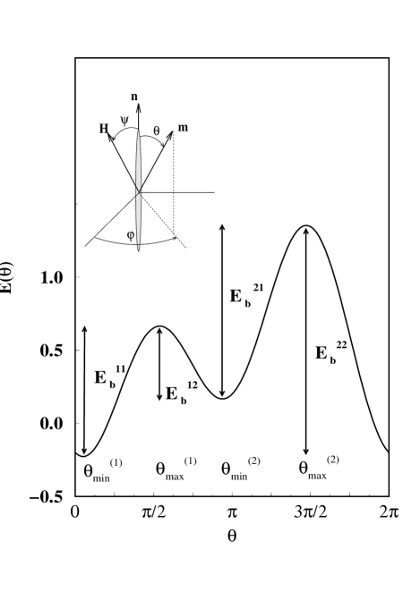
FIG. 1.: Energy function $E(\theta,\psi)$ as a function of the angle between the magnetization vector $\bf m$ and the magnetic field $\bf h$, for $\bf m$ in the plane of the easy-axis $\varphi=0$, as given by Eq. (1). The plot is for a particle whose easy-axis $\bf n$ forms an angle $\psi=30^{o}$ with $\bf h$, and $H=0.3$. We have used the following notation to designate the extrema of the energy: $\theta^{1}_{\rm min}$ and $\theta^{1}_{\rm max}$ refer to the extrema closer to the field direction while $\theta^{2}_{\rm min}$ and $\theta^{2}_{\rm max}$ refer to those further from the direction of the field. The four possible energy barriers between them are $E^{ij}_{b}\equiv E(\theta^{i}_{\rm max})-E(\theta^{j}_{\rm min})$. Inset: Schematic representation of the quantities involved in the definition of the system. The easy-axis of the particles $\bf n$ are in the x-z plane forming an angle $\psi$ with the magnetic field $\bf H$, which points along the z axis. $\theta$ and $\varphi$ are the spherical angles of the magnetization vector $\bf M$.

FIG. 2.: Upper panels: effective energy barrier distributions for aligned particles with a lognormal distribution of anisotropy constants of $\sigma=0.2$ (continuous lines), 0.5 (dashed lines), 0.8 (dot-dashed lines) for values of $H$ as indicated in the figures. Lower panels: same as upper panels but for particles with random orientations of anisotropy axes.

FIG. 3.: Magnetization curves as a function of the dimesionless Zeeman energy $\xi=\mu HV/k_{B}T$ in the TS approximation. Symbols stand for randomly oriented particles with $K_{0}=0.5,1.0,10.0$ (from the uppermost curve). The case $K_{0}=10$ is compared to the exact result given by Eq. (5)(dash-dotted line). The case $K_{0}=1$ is compared with a system of randomly oriented particles with $f(K)$, $K_{0}=1$ and $\sigma=0.5$ (long-dashed line) The result for aligned particles is displayed as a continuous line, for which $m_{TS}=\tanh(\xi)$ ($m_{\rm TS}$ is independent of $\sigma$ in this case).

FIG. 4.: Relaxation curves for an ensemble of particles with randomly oriented anisotropy axes and a logarithmic-normal distribution of anisotropies $f(K)$ of width $\sigma=0.5$ and $K_{0}=1$ calculated by numerical integration of Eq. (21). The initial magnetization has been set to $M_{0}=0$. Reduced temperatures $T/T_{0}$, starting from the lowermost curve, range from 0.01 to 0.1 with 0.01 increments, and from 0.1 to 0.2 with 0.02 increments. The applied fields are $H=0.1,0.5,1.0$ as indicated. The upper panels show the original curves normalized to the equilibrium magnetization $m_{TS}(T)$ given by Eq. (8). In the lower panels, the same curves have been plotted as a function of the scaling variable $T\ln(t/\tau_{0})$.

FIG. 5.: (a) Low temperature ($T=0.05$) viscosity curves for a system of randomly oriented particles with the same anisotropy constant $K_{0}=1$. The curves have been normalized to the equilibrium magnetization $M_{eq}(T)$ and correspond to magnetic fields $H=0.1,0.2,\dots,1.0,1.2,1.4,1.6,1.8,2.0$ increasing from right to left. (b) Field dependence of the time corresponding to the maximum relaxation rate, $T\ln(t_{max}/\tau_{0})$, as derived from the viscosity curves in panel (a) (triangles). The field dependence of the mean lowest energy barrier $E^{(2,2)}_{av}$ (diamonds), lowest energy barrier for particles oriented at $\alpha=45^{0}$, $E^{(2,2)}(\pi/4)$ (squares) and $\alpha=0$ (circles), $E^{(2,2)}(0^{0})$ are also shown for comparison. (c) Field dependence of the maximum relaxation rate $S_{max}$.

FIG. 6.: (a) Low temperature ($T=0.05$) viscosity curves for a system of particles with random orientations and logarithmic-normal distribution of anisotropies with (a) $\sigma=0.2$ and (b) $\sigma=0.5$. The curves have been normalized to the equilibrium magnetization and correspond to magnetic fields $H=0.1$ to $1.0$ in 0.1 steps and $H=1.2$ to $2.0$ in 0.2 steps starting from the right.

FIG. 7.: Upper panels: Field dependence of the energy corresponding to the maximum relaxation rate, $T\ln(t_{max}/\tau_{0})$, as derived from the viscosity curves in Fig. 6 for temperatures $T=0.01$ (circles), 0.05 (squares) , 0.1 (diamonds). Lower panels: Field dependence of the maximum relaxation rate $S_{max}$ for the same curves and temperatures. Left column is for $\sigma=0.2$ and the right one for $\sigma=0.5$.

FIG. 8.: Relaxation rates as a function of the scaling variable $T\ln(t/\tau_{0})$ for different temperatures [$T=0.01$ (dotted line), 0.05 (dashed line) , 0.1 (long-dashed line)], $\sigma=0.2$ and three magnetic fields (a) $H=0.1$, (b) $H=0.5$, and (c) $H=0.8$. The curves tend to the effective distribution of lower energy barriers $f_{\rm eff}(E^{22})$, shown as a continuous line, as $T$ decreases.

FIG. 9.: Normalized relaxation curves as a function of the scaling variable $T\ln[(t/t_{max}(h)]$ for $T=0.05$) obtained from Fig. 6 by shifting the curves in the horizontal axis with the position of the maximum relaxation rate (upper panels in Fig. 7). (a) $\sigma=0.2$ and $H=0.1,0.2,0.3,0.4,0.5$; (b) $\sigma=0.5$ and $H=0.1,0.2,0.3,0.4$ (starting from the uppermost curve)

.

REFERENCES

- [1] J. L. Dormann, D. Fiorani, and E. Tronc, Adv. Chem. Phys. 98, 283 (1997).
- [2] Proceedings of the 3rd Euroconference on Magnetic Properties of Fine Particles and their Relavance to Materials Science, edited by X. Batlle and A. Labarta, J. Magn. Magn. Mater. 221, No. 1-2, pp. 1-233 (Elsevier Science, The Netherlands, 2000).
- [3] P. C. E. Stamp, E. M. Chudnovsky, and B. Barbara, Int. J. Mod. Phys. B 6, 1355 (1992).
- [4] Quantum Tunneling of Magnetization-QTM’94, NATO Advanced Research Workshop, edited by L. Gunther and B. Barbara (Kluwer Acad. Publishers, Chichilianne, Grenoble, 1995).
- [5] E. C. Stoner and E. P. Wohlfarth, Philos. Trans. R. Soc. London A 240, 599 (1948), reprinted in IEEE Trans. Magn. 27, 3475 (1991).
- [6] L. Néel, Ann. Géophys. 5, 99 (1949).
- [7] R. Street and J. C. Wooley, Phys. Soc. A 62, 562 (1949).
- [8] R. W. Chantrell, J. Magn. Magn. Mater. 95, 365 (1991).
- [9] E. P. Wohlfarth, J. Phys. F 14, L155 (1984).
- [10] R. W. Chantrell, M. Fearon, and E. P. Wohlfarth, Phys. Stat. Sol. 97, 213 (1986).
- [11] A. M. de Witte, K. O’Grady, G. N. Coverdale, and R. W. Chantrell, J. Magn. Magn. Mater. 88, 183 (1990).
- [12] D. Givord, A. Lienard, P. Tenaud, and T. Viadieu, J. Magn. Magn. Mater. 67, L281 (1987).
- [13] D. Givord, P. Tenaud, and T. Viadieu, J. Magn. Magn. Mater. 72, 247 (1988).
- [14] A. Labarta, O. Iglesias, Ll. Balcells, and F. Badia, Phys. Rev. B 48, 10240 (1993).
- [15] O. Iglesias, F. Badia, A. Labarta, and Ll. Balcells, J. Magn. Magn. Mater. 140-144, 399 (1995).
- [16] O. Iglesias, F. Badia, A. Labarta, and Ll. Balcells, Z. Phys. B 100, 173 (1996).
- [17] Ll. Balcells, O. Iglesias, and A. Labarta, Phys. Rev. B 55, 8940 (1997).
- [18] B. Barbara and L. Gunther, J. Magn. Magn. Mater. 128, 35 (1993).
- [19] E. Vincent, J. Hammann, P. Prené, and E. Tronc, J. Phys. I France 4, 273 (1994).
- [20] W. Wernsdorfer et al., J. Magn. Magn. Mater. 145, 33 (1995).
- [21] P. L. Kim, C. Lodder, and T. Popma, J. Magn. Magn. Mater. 193, 249 (1999).
- [22] A. Lisfi et al., J. Magn. Magn. Mater. 193, 258 (1999).
- [23] I. D. Mayergoyz et al., J. Appl. Phys. 85, 4358 (1999).
- [24] M. G. del Muro, X. Batlle, and A. Labarta, Phys. Rev. B 59, 13584 (1999).
- [25] D. V. Berkov, J. Magn. Magn. Mater. 111, 327 (1992).
- [26] R. H. Victora, Phys. Rev. Lett. 63, 457 (1991).
- [27] P. J. Cregg and L. Bessais, J. Magn. Magn. Mater. 203, 265 (1999).
- [28] R. W. Chantrell, N. Y. Ayoub, and J. Popplewell, J. Magn. Magn. Mater. 53, 199 (1985).
- [29] H. Pfeiffer, Phys. Stat. Sol. A 120, 233 (1990).
- [30] H. Pfeiffer, Phys. Stat. Sol. A 122, 377 (1990).
- [31] J. L. García-Palacios, Adv. Chem. Phys. 112, 1 (2000).
- [32] W. F. Brown, Jr., Phys. Rev. 130, 1677 (1963).
- [33] W. T. Coffey, Y. P. Kalmykov, and J. T. Waldron, The Langevin equation : with applications in physics, chemistry and electrical engineering (World Scientific, Singapore, 1996).
- [34] U. Wolff, Phys. Rev. Lett. 62, 361 (1989).
- [35] A. Lyberatos, J. Phys. D: Appl. Phys. 33, R117 (2000).
- [36] U. Nowak, Ann. Rev. of Comp. Phys. 9, 105 (2001).
- [37] P. Milténi et al., Phys. Rev. Lett. 84, 4224 (2000).
- [38] F. Reif, Fundamentals of Statistical and thermal dynamics (Mc Graw Hill, New York, 1967).
- [39] J. M. González, R. Ramírez, R. Smirnov-Rueda, and J. González, Phys. Rev. B 52, 16034 (1996).
- [40] L. C. Sampaio, C. Paulsen, and B. Barbara, J. Magn. Magn. Mater. 140-144, 391 (1995).
- [41] A. Marchand, L. C. Sampaio, and B. Barbara, J. Magn. Magn. Mater. 140-144, 1863 (1994).
- [42] R. Sappey et al., Phys. Rev. B 56, 14551 (1997).
.