Towards the Evaluation of
the Relevant Degrees of Freedom in
Nonlinear Partial Differential Equations

Abstract

We investigate an operator renormalization group method to extract and describe the relevant degrees of freedom in the evolution of partial differential equations. The proposed renormalization group approach is formulated as an analytical method providing the fundamental concepts of a numerical algorithm applicable to various dynamical systems. We examine dynamical scaling characteristics in the short-time and the long-time evolution regime providing only a reduced number of degrees of freedom to the evolution process.

PACS Numbers:  02.30.Jr ,  02.60.Cb ,  05.45.-a ,  05.10.Cc ,  64.60.Ak ,  64.60.Ht

KEY WORDS: Renormalization group; coarse-graining; nonlinear evolutionary dynamics; partial differential equations.

1 Introduction

Based on the arguments of L.P. Kadanoff [1], K.G. Wilson developed a (numerical) renormalization group (RG) approach in the context of critical phenomena [2] and later used the developed formalism to solve the Kondo problem [3]. In practical RG applications to systems with many degrees of freedom a RG transformation is established for a stepwise elimination of the irrelevant degrees of freedom in the system. The universality of the critical behaviour of the physical system emerges in the RG approach in a natural way, with a set of universal exponents for each universality class.
Soon after the considerable success of the RG for equilibrium systems a generalization of the method was introduced to handle dynamic properties of spin systems [4]. The goal was to obtain critical exponents for stochastic equations and the developed generalization of the Wilson’s equilibrium theory has become known as the dynamic RG (DRG) method for non-equilibrium systems [5]. The DRG method, inherently defined as a Fourier space technique, was further developed and improved by other authors including D. Forster, D. Nelson and M. Stephen who studied the dynamics of the noisy Burgers equation [6]. In 1986 Burgers equation was transformed into the language of growth processes by M. Kardar, G. Parisi and Y.-C. Zhang [7] later called the KPZ equation. Applying the DRG to the KPZ equation the corresponding universal critical exponents were derived perturbatively within various higher order expansions [8, 9].
However, the impact of dimensionality on applying the DRG method to the KPZ or the related Burgers equation is crucial [10]. For dimension $d>1$ the exhibited strong coupling RG flow behaviour is not accessible by perturbative expansions and the standard approaches fail to calculate critical exponents [11]. New analytic approximations were proposed [12] including RG methods based on technical variations or combining different approaches like perturbation and scaling techniques [13]. Furthermore numerical simulation techniques were developed to allow for estimating the critical exponents [14, 15] although these approaches can suffer from numerical instabilities [16].
Contrary non-perturbative Real-Space RG techniques have been proven to produce accurate results within strong-coupling regimes [17, 18] and therefore offer, in principle, the possibility to study models that belong to the KPZ universality class. Why is it then that currently no satisfying generally applicable Real-Space RG approach is available for dynamical systems as this is the case for their equilibrium counterparts? In the following we would like to answer this question in detail and we propose a list of the fundamental problems arising in the context.
Many of the modern Real-Space RG (RSRG) methods for strong-coupled systems use an operator formalism to define the RG transformation (RGT) [19, 20] which under iterative application defines the RG flow. The RGT in the operator formalism is formally based on the application of two linear maps, a truncation or fine-to-coarse operator and an embedding or coarse-to-fine operator [20, 21]. Usage of these two operators should be sufficient for the construction of renormalized or effective quantities. Within the equilibrium operator RSRG an effective observable, including in particular the Hamiltonian, is defined by first applying the coarse-to-fine operator followed by the original observable. Finally the fine-to-coarse operator is used as a map back on the effective vector-space.
Recently N. Goldenfeld, A. McKane and Q. Hou investigated the use of operator RSRG methods to solve partial differential equations (PDEs) numerically [22] and carried on their ideas in a further paper [23]. In their work the authors generalized the operator concept of the RSRG to non-equilibrium system by replacing the equilibrium Hamiltonian operator by the time evolution operator of a partial differential equation. However the authors showed that such an approach is, in principle, not well-defined. Furthermore the proposed approach is less systematic and unsatisfactory for several reasons. Here we summarize the concerns of Goldenfeld et al and complete the list by considerations of the present authors.

1. Neither the coarse-to-fine operator nor the fine-to-coarse operator are uniquely defined. The chosen coarse-graining procedure does not depend on the specific dynamical system.

2. The coarse-to-fine operator and the time evolution operator do not commute in general. Therefore no consistent and well defined RSRG operator formalism can be established.

3. The geometric construction of the coarse-to-fine operator is unsatisfactory since it assumes the relevant degrees of freedom to be distributed within the long wavelength fluctuations. This is not necessarily the case for the evolution of many degrees of freedom interacting through nonlinear dynamics.

4. Instead of coarse-graining the governing PDE in a systematic procedure, the provided initial field configuration at time $t=0$ is coarse-grained with respect to a larger lattice spacing. Evolving a coarse-grained field configuration is not equivalent to successive RGTs removing the relevant degrees of freedom in time.

5. In a practical application of the operator concept introduced by Goldenfeld et al the coarse-graining procedure and the time evolution procedure are successive operations. However, performing an equilibrium RG step followed by an evolution of the system in time is, in general, not equivalent to a dynamic RG step.

6. The proposed operator scheme does not allow to calculate the distribution of the relevant degrees of freedom in a dynamical system. Accordingly, RG flow equations do not yield any insight to the relevant physics of the system.

In our previous work [24], which can be considered as a further development of the work of Goldenfeld et al [22], we developed a consistent and mathematically well defined RSRG operator approach. The basic concepts also used in this article are briefly summarized in section 2 and generalized by including time evolution operators. In our previous work we used the introduced operator formalism to construct the embedding and truncation maps by a quasi-static geometric coarse-graining. The conceptional disadvantage of a geometric approach is that it inherently integrates out the small scales which, because of scale interference in the evolutionary process, are not necessarily the scales one wishes to ignore [22]. However, the technique can be easily applied to a great variety of physical problems, even if defined on very large lattices.
The essential difference in the approach proposed here is a non-geometric construction of the coarse-to-fine and fine-to-coarse operators involving the evolution dynamics of the particular PDE of interest. In this work we solve all reported problems summarized above and calculate observables to determine the universal characteristics in a class of nonlinear PDEs. As a non-geometric generalization of our earlier RSRG operator approach the proposed method provides a non-perturbative real-space RG analogue to the DRG Fourier space method.
We continue to present the fundamental concepts of the non-geometric RSRG operator approach in section 3. In particular, we develop two concepts applicable in the short and long time regime of the evolutionary dynamics respectively. In section 4 we solve the linear diffusion problem exactly and present an analytic construction scheme for the coarse-to-fine and fine-to-coarse operator. We continue in section 5 by generalizing the method as a numerical algorithm applicable to nonlinear evolution equations in general. Using transformations which are local in time allows for exact mapping of the non-linear dynamics to linear evolution dynamics governed by the diffusion equation.
In this work we denote the dependence of a function $f$ on spatial variables $x$ and temporal variables $t$ as $f(x,t)$. Contrarily the spatial and temporal dependence of a discretized function $f$ will be denoted by indexing sets $i,i+1,\dots$ and $t,t+1,\dots$ respectively. Here $i,i-1$ and $i,i+1$ refer to neighbouring sites in the lattice whereas $t-1,t,t+1$ denote successive time steps. Not necessarily neighbouring sites are denoted as $i,j$ and by using capital letters $I,J$ we refer to the sites of the effective lattice. Quantities defined in this effective vector space are equipped with a prime. A set of vectors is denoted as $\{\mathinner{|{{\bf v}_{i}}\rangle}\}_{i=M}^{N}$ where the indexing set starts at $i=M$ and extends to $i=N$.

2 The Operator Real-space RG Approach

In this work we consider examples of evolution equations of the form

$$\partial_{t}\phi\;=\;\tilde{H}\phi,$$ (1)

with $\phi=\phi(x,t)$ a function of space $x$ and time $t$ and the operator $\tilde{H}$ acting as the generator of the evolution. Although every operator $\tilde{H}$ acting locally in time can be considered, we restrict our calculations for clarity to linear and quadratic evolution operators, $H$ and $Q$ respectively,

$$\tilde{H}\;=\;(H+Q)\;.$$ (2)

Discretizing equation (1) in space and time using (2) yields

$${\phi}_{i,t+\Delta t}\;=\;\sum_{j=1}^{N}({\mathbbm{1}_{i,j}}+\Delta t\,\cdot\,H_{i,j})\phi_{j,t}\,+\,\Delta t\,\sum_{j,k=1}^{N}\,Q_{i,j,k}\phi_{j,t}\phi_{k,t}\;\,:=\;f_{i}\left[{\bf\phi}_{t}\right]$$ (3)

with $i\in\{1,\dots,N\}$ and $N$ denoting the number of sites in the lattice. The spatial lattice spacing is denoted as $\Delta x$ and the discrete temporal integration interval as $\Delta t$. The function ${\bf\phi}_{t}$ defines a vector in a vector space $V^{N}$ and the functional $f\left[{\bf\phi}_{t}\right]$ defined in (3) is a map

(6)

Using this vector space notation the concept of a truncation or fine-to-coarse operator $G$ together with an embedding or coarse-to-fine operator $G^{p}$ is provided by the not necessarily commuting diagram

(11)

Here the truncation operator $G$ is defined by the relation

$${\bf\phi}^{\prime}_{I}\;=\;\sum_{i=1}^{N}\,G_{I,i}\,{\bf\phi}_{i}\;,$$ (12)

where capital indexing letters $I\in\{1,\dots,M\}$ refer to lattice sites in the effective vector space $V^{M}$. If $M=N$ and ${\rm Ker}(G)=\emptyset$, the embedding operator $G^{p}$ may be chosen as the natural inverse of the truncation operator $G$ defined as

$${\bf\phi}_{i}\;=\;\sum_{I=1}^{M}\,G^{p}_{i,I}\,{\bf\phi}^{\prime}_{I}\;=\;\sum_{I=1}^{M}\,G^{-1}_{i,I}\,{\bf\phi}^{\prime}_{I}$$ (13)

and the diagram (11) commutes.
However, within practical applications the idea is to choose $M<N$ and replace equation (3) with a coarse grained evolution equation providing less degrees of freedom. Considering $G$ as a projector on the relevant degrees of freedom the inverse operator $G^{-1}$ does not exist. This naturally demands for a generalized definition of the embedding operator $G^{p}$ as the pseudo-inverse

$${\bf\phi}_{i}\;=\;\sum_{I=1}^{M}\,G^{p}_{i,I}\,{\bf\phi^{\prime}}_{I}$$ (14)

calculated by Singular Value Decomposition (SVD) [25]. For $M<N$ the functional $f^{\prime}\left[{\bf\phi}^{\prime}_{t}\right]$ is defined as in (3) on an effective lattice with a reduced number of lattice sites $M$

(17)

$$\mbox{and}\qquad\lx@xy@svg{\hbox{\raise 0.0pt\hbox{\kern 10.76631pt\hbox{\ignorespaces\ignorespaces\ignorespaces\hbox{\vtop{\kern 0.0pt\offinterlineskip\halign{\entry@#!@&&\entry@@#!@\cr&\crcr}}}\ignorespaces{\hbox{\kern-10.76631pt\raise 0.0pt\hbox{\hbox{\kern 0.0pt\raise 0.0pt\hbox{\hbox{\kern 1.0pt\raise 0.0pt\hbox{$\textstyle{{\phi^{\prime}}_{I,t}\;\;\ignorespaces\ignorespaces\ignorespaces\ignorespaces}$}}}}}}}\ignorespaces\ignorespaces\ignorespaces\ignorespaces{\hbox{\kern 10.76633pt\raise 0.0pt\hbox{\hbox{\kern 0.0pt\raise 0.0pt\hbox{\lx@xy@stopper}}}}}{\hbox{\lx@xy@droprule}}\ignorespaces{\hbox{\kern 34.76631pt\raise 0.0pt\hbox{\hbox{\kern 0.0pt\raise 0.0pt\hbox{\lx@xy@tip{1}\lx@xy@tip{-1}}}}}}{\hbox{\lx@xy@droprule}}{\hbox{\lx@xy@droprule}}{\hbox{\kern 34.76631pt\raise 0.0pt\hbox{\hbox{\kern 0.0pt\raise 0.0pt\hbox{\hbox{\kern 1.0pt\raise 0.0pt\hbox{$\textstyle{\;\;{\phi^{\prime}}_{I,t+\Delta t}}$}}}}}}}\ignorespaces}}}}\ignorespaces\;=\;\sum_{J=1}^{M} \textstyle{{\phi^{\prime}}_{I,t}\;\;\ignorespaces\ignorespaces\ignorespaces\ignorespaces} \textstyle{\;\;{\phi^{\prime}}_{I,t+\Delta t}} \textstyle{{\phi^{\prime}}_{I,t}\;\;\ignorespaces\ignorespaces\ignorespaces\ignorespaces} \textstyle{\;\;{\phi^{\prime}}_{I,t+\Delta t}} \left({\mathbbm{1}}_{I,J}+\Delta t\,\cdot\,H^{\prime}_{I,J}\right){\phi^{\prime}}_{J,t}$$ (20)

$$+\,\Delta t\sum_{J,K=1}^{M}\,Q^{\prime}_{I,J,K}{\phi^{\prime}}_{J,t}{\phi^{\prime}}_{K,t}\;.$$ (21)

In equation (20) $H^{\prime}$ and $Q^{\prime}$ denote the effective linear and quadratic evolution operators defined as [24]

$$H^{\prime}_{I,J}\;:=\;G_{I,i}\,H_{i,j}\,G^{p}_{j,J}\qquad\mbox{and}\qquad Q^{\prime}_{I,J,K}\;:=\;G_{I,i}\,Q_{i,j,k}\,G^{p}_{j,J}\,G^{p}_{k,K}\;\;.$$ (22)

Inserting (12), (14) and (20) into the non-commuting diagram (11) we replace equation (3) by an approximate field evolution equation on a coarse grained lattice as

$${\phi}_{i,t+\Delta t} \;\approx\;\sum_{j=1}^{N}\sum_{J=1}^{M}G^{p}_{i,I}({\mathbbm{1}}_{I,J}+\Delta t\cdot H^{\prime}_{I,J})G_{J,j}\phi_{j,t}$$

$$\qquad\quad+\Delta t\sum_{j,k=1}^{N}\sum_{J,K=1}^{M}G^{p}_{i,I}\,Q^{\prime}_{I,J,K}\,G_{J,j}G_{K,k}\,\phi_{j,t}\phi_{k,t}$$

$$\;=\;\Big{[}\;G^{p}\left({\mathbbm{1}}\,+\,\Delta t\cdot H^{\prime}\,+\,\Delta t\cdot Q^{\prime}\right)G\,{\bf\phi}_{t}\;\Big{]}_{i}\quad,$$ (23)

describing the evolution of the field ${\bf\phi}$ under a reduced number of degrees of freedom.
Equation (2) defines a RG transformation (RGT) within the operator formalism and iterating the RGT defines a RG flow. Carrying out one RGT is called a RG step (RGS) and according to the concept developed in this section is equivalent to an approximate field evolution using less degrees of freedom. Equation (2) defines the real-space analogue of a RGT established within the DRG method. The field itself provides the set of parameters used to establish a RGT [20]. Furthermore, equation (2) fuses the coarse-graining and the time evolution procedure and provides a solution to the problem number 5 formulated in the introduction.

3 Non-geometric reduction of the degrees of freedom

In this section we provide a general concept for reducing the degrees of freedom in evolutionary systems without geometrically coarse-graining the lattice equations. Including the temporal characteristics of the particular partial differential equation (PDE) into the construction of the embedding and truncation operators we distinguish between a short-time regime and a long-time regime.

3.1 Short-time evolution

Within the short-time regime we describe the evolution of the field as a perturbation of the initial field configuration at time $t=0$. Evolving the initial field ${\bf\phi}_{0}$ for $M$ time steps $\Delta t$ the dynamics within this short-time interval is conserved by the set of vectors

$${\cal S}\;:=\;\{{\bf\phi}_{0},{\tilde{H}}{\bf\phi}_{0},{\tilde{H}}^{2}{\bf\phi}_{0},\ldots,{\tilde{H}}^{M-1}{\bf\phi}_{0}\}$$ (24)

where ${\tilde{H}}$ is the evolution operator defined in (2). Using the set of vectors in (24) as the columns and rows of the linear operators $G$ and $G^{p}$ (previously orthonormalized), these can be considered as projection maps from and into the space $V^{M}$ respectively.
If $M\leq N$ the relation

$${\bf\phi}_{t}\;=\;G^{p}\left({\mathbbm{1}}+\Delta t\tilde{H}^{\prime}\right)^{M}G\,{\bf\phi}_{0}\qquad\mbox{with}\quad\tilde{H}^{\prime}\;=\;H^{\prime}\,+\,Q^{\prime}$$ (25)

governs an exact evolution of the field ${\bf\phi}_{t}$ on the effective coarse-grained lattice for $t<M\Delta t$. In this case the states in (24) span a subspace $V^{M}$ of the full vector-space $V^{N}$ conserving the relevant degrees of freedom for the short-time evolutionary regime. In the considered short-time regime, we may rewrite equation (25) as

$${\bf\phi}_{t}\;=\;\left[\;G^{p}\left({\mathbbm{1}}+\Delta t\tilde{H}^{\prime}\right)G\;\right]^{M}\,{\bf\phi}_{0}$$ (26)

which determines a RG flow in the short time regime and a RGS is defined by relation (2).
However, if $t\geq M\Delta t$ equation (26) is an approximation to the evolved field ${\bf\phi}_{t}$. In this case the approach is only applicable if no relevant scale interference in the evolutionary process occurs. This is unlikely the case for longer times in nonlinear dynamical systems and relation (26) becomes a crude approximation giving rise to numerical instabilities.

3.2 Long-time evolution

Nonlinear evolution processes exhibit most of their characteristics in the long-time regime. The asymptotic form of the field or surface configuration in growth phenomena [7] or the formation of turbulent states out of spiral waves [34] are only two examples. This gives rise to a reduction scheme for the degrees of freedom of a dynamical system valid in the long-time asymptotics. This in turn demands for new concepts in the construction of the embedding and truncation operators $G^{p}$ and $G$ away from any initial field configuration.
Therefore our task is to minimize the magnitude of the non-commutativity in the diagram (11) for all times of the evolution process. This in turn rises the important question if such a minimum exists and if a numerical algorithm will uniquely converge. To measure the non-commutativity in the diagram (11) we calculate the difference between the approximately evolved field using a reduced number of degrees of freedom and the exactly evolved field as

$${\cal E}{\bf\phi}_{t}\;:=\;({\mathbbm{1}}+\Delta t\tilde{H}){\bf\phi}_{t}\,-\,(G^{p})({\mathbbm{1}}+\Delta t\tilde{H}^{\prime})G\,{\bf\phi}_{t}\;\;.$$ (27)

We call ${\cal E}$ the error operator and generalize the operator concept introduced in section 2 according to the commutative diagram

(32)

The introduced minimization concept is one of the fundamental principles in equilibrium operator RSRG techniques [17, 21]. Using the established notation in the formulation of the dynamic operator RSRG, $({\mathbbm{1}}+\Delta tH){\bf\phi}_{t}$ is called the target state [17] and $(G^{p})({\mathbbm{1}}+\Delta t\tilde{H}^{\prime})G\,{\bf\phi}_{t}$ an optimal representation of the target state [17] in the subspace $V^{M}\subset V^{N}$.
We are interested in the limit ${\cal E}{\bf\phi}_{t}\rightarrow 0$ for $t\gg 0$ subject to any field configuration ${\bf\phi}_{0}$. To exclude the explicit field dependence from the minimization procedure we rewrite equation (27) in operator form as

$${\cal E}\;=\;({\mathbbm{1}}+\Delta tH)\,-\,G^{p}(1+\Delta t\tilde{H}^{\prime})G\;\;.$$ (34)

To make this operator as small as possible we minimize ${\cal E}$ in the matrix notation according to the Frobenius norm . Inserting the definitions (22) we rewrite equation (34) using the Frobenius norm $||_{F}$ as

$$|{\cal E}|_{F}\;:=\;\left\{{\mathbbm{1}}-(G^{p}G)+\Delta t\Big{[}H-(G^{p}G)\,\tilde{H}\,(G^{p}G)\Big{]}\right\}^{2}\;\;.$$ (35)

The measured magnitude of the non-commutativity in the original diagram (11) has become a number $|{\cal E}|_{F}$ greater or equal to zero. According to equation (35) the minimization of the error operator ${\cal E}$ only depends on the composed operator $G^{p}G$. Therefore two different $G$ matrices for which $G^{p}G$ is the same operator yield the same error number $|{\cal E}|_{F}$.
The matrix $G^{p}G$ is called the reduction operator since it governs the field evolution under a reduced number of degrees of freedom. To make this more obvious we rewrite $G$ and $G^{p}$ in terms of a Singular Value Decomposition

$$G\;=\;\sum_{i=1}^{M}\lambda_{i}\mathinner{|{{\bf u}_{i}}\rangle}\mathinner{\langle{{\bf v}_{i}}|}\qquad\mbox{and}\qquad G^{p}\;=\;\sum_{i=1}^{M}\lambda^{-1}_{i}\mathinner{|{{\bf v}_{i}}\rangle}\mathinner{\langle{{\bf u}_{i}}|}\;,$$ (36)

where $\{\mathinner{|{{\bf v}_{i}}\rangle}\}_{i=1}^{M}$ and $\{\mathinner{|{{\bf u}_{i}}\rangle}\}_{i=1}^{M}$ are respectively sets of $N$-dimensional and $M$-dimensional vectors. By means of (36) we define the reduction operator as

$${\cal R}\;:=\;G^{p}G\;=\;\sum_{i=1}^{M}\mathinner{|{{\bf v}_{i}}\rangle}\mathinner{\langle{{\bf v}_{i}}|}\;.$$ (37)

In this notation the reduction operator ${\cal R}$ is composed of $M$ states and acts on the original vector space $V^{N}$, with $N>M$. Since there are some states $\{\mathinner{|{{\bf v}_{i}}\rangle}\}_{i=M+1}^{N}$ which together with $\{{\bf v}_{i}\}_{i=1}^{M}$ represent a whole orthonormal basis of $V_{N}$, the reduction operator ${\cal R}$ projects out those states representing the less relevant degrees of freedom in the evolution process.
We would like to point out that different truncation operators $G$ can be used to construct the same reduction operator ${\cal R}=G^{p}G$. In fact every RSRG approach requires a correct choice of the RG transformation (RGT) which is not uniquely defined. In the operator formalism the embedding and truncation operators are used to construct the RGT [20]. In the dynamic operator RSRG method introduced in this work, the RGT is defined as one time step in the field evolution equation (2). From this point of view all truncation operators yielding the same reduction operator ${\cal R}$ represent an error equivalence class as far as the evolution error is the only concern. Other computational considerations, such as the sparseness of the $\tilde{H}$ matrix shall force us to choose one or another truncation operator.
Before we discuss the field evolution according to the reduction operator ${\cal R}$ we would like to give a remark concerning the structure of equation (35). Choosing $\Delta t=0$, i.e. no dynamics is involved, equation (35) reduces to the geometric operator real space RG approach [24]. For $\Delta t>0$ the third summand on the right hand side includes the evolution operator of the particular PDE into the minimization process. Furthermore this term is weighted by the time interval $\Delta t$. Therefore the particular evolution operator is included into the minimization process and resulting relevant degrees of freedom for the evolutionary dynamics can depend on the chosen time interval.
To reformulate the approximate field evolution in terms of the reduction operator we insert the definitions (22) and (37) into (2) resulting in

$${\phi}_{i,t+\Delta t}\;=\;{\cal R}\left[{\phi}_{t}+\Delta t\,\cdot\,\right(H+Q\left)\,{\cal R}\,{\phi}_{t}\right]\;.$$ (38)

Within practical calculations the process of constructing ${\cal R}$ can be decomposed according to successive dimensional reduction of the target space

(41)

Within the first dimensional reduction we have to minimize (35) by adjusting the $N$ components of the vector $\mathinner{|{{\bf v}_{N}}\rangle}$ which defines the first order reduction operator as

$${\cal R}^{1}\;:=\;\sum_{i=1}^{N-1}\mathinner{|{{\bf v}_{i}}\rangle}\mathinner{\langle{{\bf v}_{i}}|}\;=\;{\mathbbm{1}}-\mathinner{|{{\bf v}_{N}}\rangle}\mathinner{\langle{{\bf v}_{N}}|}\;,$$ (42)

where we used the notation of relation (37). Analogously we calculate the second order reduction operator as

$${\cal R}^{2}\;:=\;\sum_{i=1}^{N-2}\mathinner{|{{\bf v}_{i}}\rangle}\mathinner{\langle{{\bf v}_{i}}|} \;=\;{\mathbbm{1}}-\mathinner{|{{\bf v}_{N}}\rangle}\mathinner{\langle{{\bf v}_{N}}|}-\mathinner{|{{\bf v}_{N-1}}\rangle}\mathinner{\langle{{\bf v}_{N-1}}|}$$

$$\;=\;{\cal R}^{1}-{\cal P}_{\mathinner{|{{\bf v}_{N-1}}\rangle}}\;.$$ (43)

In (3.2) we have introduced the notation of the projection operator ${\cal P}_{\mathinner{|{\bf v}\rangle}}$ defined as the projection map ${\cal P}_{\mathinner{|{\bf v}\rangle}}=(\mathinner{|{\bf v}\rangle}\mathinner{\langle{\bf v}|})$ onto the state $\mathinner{|{\bf v}\rangle}$.
Iterating up to the $M$th order the reduction operator is calculated as

$${\cal R}^{M}\;=\;{\cal R}^{M+1}-\mathinner{|{{\bf v}_{N+1-M}}\rangle}\mathinner{\langle{{\bf v}_{N+1-M}}|}\;=\;{\cal R}^{M+1}-{\cal P}_{\mathinner{|{{\bf v}_{N+1-M}}\rangle}}\;,$$ (44)

with ${\cal R}^{0}={\mathbbm{1}}$. In equation (44) we have denoted by ${\cal P}_{\mathinner{|{{\bf v}_{N+1-M}}\rangle}}$ the projection operator onto the state $\mathinner{|{{\bf v}_{N+1-M}}\rangle}$ which is the target to calculate in the $M$th minimization procedure.
Similar calculations can be performed for the error operator ${\cal E}$. Using the abbreviation $\mathinner{|{\bf v}\rangle}:=\mathinner{|{\bf v}\rangle}_{N}$ the error operator for the first dimensional reduction is defined as

$${\cal E}^{1}\; =\;{\mathbbm{1}}-({\mathbbm{1}}-\mathinner{|{v}\rangle}\mathinner{\langle{v}|})+\Delta t\Big{[}\,\tilde{H}-({\mathbbm{1}}-\mathinner{|{v}\rangle}\mathinner{\langle{v}|})\,\tilde{H}\,({\mathbbm{1}}-\mathinner{|{v}\rangle}\mathinner{\langle{v}|})\,\Big{]}$$

$$=\;{\cal P}_{\mathinner{|{v}\rangle}}+\Delta t\Big{(}\,\tilde{H}{\cal P}_{\mathinner{|{v}\rangle}}+{\cal P}_{\mathinner{|{v}\rangle}}\tilde{H}-\mathinner{\langle{v}|}\tilde{H}\mathinner{|{v}\rangle}{\cal P}_{\mathinner{|{v}\rangle}}\,\Big{)}\;\;.$$ (45)

Using the iterative scheme (44) we write the minimization procedure for the state $\mathinner{|{{\bf v}_{N+1-M}}\rangle}$ as

$$|{\cal E}^{M}|_{F}\; =\;{\mathbbm{1}}-{\cal R}^{M}+\Delta t\Big{(}\,\tilde{H}\,-\,{\cal R}^{M}\,\tilde{H}\,{\cal R}^{M}\,\Big{)}\;.$$ (46)

According to relation (46) we call a truncation of the original vector space $V^{N}$ an order $M$ truncation or a reduction of order $M$ in the degrees of freedom. The ratio

$$\lambda\;:=\;N/(N-M)$$ (47)

is defined as the reduction factor $\lambda$.

4 An Exactly Solvable Lattice Model

In this section we treat the special case $\tilde{H}=H$, i.e. a linear evolution dynamics. For both a selfadjoint and a non-selfadjoint evolution operator the reduction operator can be calculated exactly up to an arbitrary order in dimensional reduction of the original vector space $V^{N}$. As an example for a selfadjoint linear evolution operator we examine the diffusion equation given by

$$\frac{\partial{\bf w}(x,t)}{\partial t}\;=\;\nu\cdot{\nabla}^{2}{\bf w}(x,t)\;,$$ (48)

where the diffusion coefficient $\nu$ describes the strength of the relaxation process.
In figure 1 we evolved the initial field configuration (dashed line) according to the method described in section 3.1 for a total time $t=100$ and $t=1000$.

   

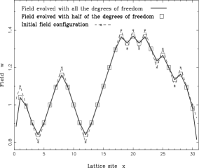
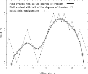
Figure 1: The initial and the evolved fields for a lattice composed of 32 sites after 100 and 1000 time steps (a) and (b) respectively. The initial field configuration is drawn by the dashed curve. The fields were evolved using a time interval $\Delta t=1$ and a diffusion parameter $\nu=0.01$. The numerical minimization was performed up to the 16th order reduction in the degrees of freedom equivalent to a reduction factor of $\lambda=2$.

The solid curve shows the field evolution on the original lattice composed of 32 sites. The field evolved with half of the degrees of freedom corresponding to an evolution on a lattice composed of 16 sites is displayed by a $\,\square\,$ for every lattice site. The embedding and truncation operators $G^{p}$ and $G$ were composed according to (24) with M=16. For the numerical evolution of equation (48) we consider the following discrete differencing of (48)

$$\frac{{\bf w}_{i,t+\Delta t}\,-\,{\bf w}_{i,t}}{\Delta t}\;=\;\nu\cdot\left[\,\frac{{\bf w}_{i+1,t}\,-\,2{\bf w}_{i,t}\,-\,{\bf w}_{i-1,t}}{\left({\Delta t}\right)^{2}}\,\right]\;.$$ (49)

In equation (49) we used a forward Euler scheme in time [25] and the linear evolution operator $H$ is defined as

$$H_{i,j}\;:=\;\left(\nu\cdot{\nabla}^{2}\right)_{i,j}\;:=\;\begin{cases}\,-2\nu/{\left({\Delta t}\right)^{2}}&\quad\mbox{if}\;i=j\\ \quad\nu/{\left({\Delta t}\right)^{2}}&\quad\mbox{if}\;j\;\mbox{nearest neighbour site of}\;i\\ \quad\;0&\quad\mbox{else}\;.\end{cases}$$ (50)

From figure 1 it is obvious that the evolution under a reduced number of degrees of freedom does not differ from the evolution of the field using all degrees of freedom. Even for longer evolution times which corresponds to equation (26) with $M\gg N$ the field evolved with half of the degrees of freedom does not differ from the exact evolution. This indicates that the relevant degrees of freedom can already be deduced from the early time dynamics. Therefore the degrees of freedom do not mix in linear evolution, i.e. small scale dynamics and large scale dynamics do not interfere.
To calculate the long-time evolution characteristics we have to minimize $|{\cal E}|_{F}$ in (35) by iterative application of (46) according to (44). We diagonalize the self-adjoint operator $H$ according to the orthonormal basis $\{\mathinner{|{u_{i}}\rangle}\}_{i=1}^{N}$ with real eigenvalues $E_{i}$ given by

$$H\;=\;\sum_{i=1}^{N}E_{i}\mathinner{|{u_{i}}\rangle}\mathinner{\langle{u_{i}}|}\;.$$ (51)

The eigenvalues $E_{i}$ are supposed to be real and in increasing order: $E_{1}\leq E_{2}\leq\ldots\leq E_{N}$. If the basis $\{\mathinner{|{u_{i}}\rangle}\}_{i=1}^{N}$ is orthonormal the vector $\mathinner{|{v}\rangle}$ in (3.2) can be decomposed according to

$$\mathinner{|{v}\rangle}\;=\;\sum_{j=1}^{N}\mu_{j}\mathinner{|{u_{j}}\rangle}\;,$$ (52)

where we are assuming $\mu_{i}\in{\mathbbm{R}}$ for all $i$. Using relation (52) the different summands in equation (3.2) can be calculated explicitly as

$${\cal P}_{\mathinner{|{v}\rangle}} \;=\;\sum_{i,j=1}^{N}\mu_{i}\mu_{j}\mathinner{|{u_{i}}\rangle}\mathinner{\langle{u_{j}}|}\qquad\quad\mathinner{\langle{v}|}H\mathinner{|{v}\rangle}\;=\;\sum_{i=1}^{N}\mu_{i}^{2}E_{i}\;\equiv\;\mathinner{\langle{H}\rangle}$$

$$H{\cal P}_{\mathinner{|{v}\rangle}} \;=\;\sum_{i,j=1}^{N}\mu_{i}\mu_{j}E_{i}\mathinner{|{u_{i}}\rangle}\mathinner{\langle{u_{j}}|}\qquad\quad{\cal P}_{\mathinner{|{v}\rangle}}H\;=\;\sum_{i,j=1}^{N}\mu_{i}\mu_{j}E_{j}\mathinner{|{u_{i}}\rangle}\mathinner{\langle{u_{j}}|}$$ (53)

and relation (3.2) becomes

$${\cal E}_{ij}\;=\;\Big{[}\,{\mathbbm{1}}+\Delta t\left(E_{i}+E_{j}-\mathinner{\langle{H}\rangle}\right)\,\Big{]}\mu_{i}\mu_{j}\;.$$ (54)

According to definition (35) we have to minimize

$$|{\cal E}|_{F}\;=\;\sum_{i,j=1}^{N}\Big{[}\,{\mathbbm{1}}+\Delta t\left(E_{i}+E_{j}-\mathinner{\langle{H}\rangle}\right)\,\Big{]}^{2}\mu_{i}^{2}\mu_{j}^{2}\;.$$ (55)

Expanding into explicit summands and retaining only terms which are first order in $\Delta t$ this yields

$$|{\cal E}|_{F}\;=\;1\;+\;2\Delta t\mathinner{\langle{H}\rangle}\;.$$ (56)

Therefore $\mathinner{\langle{H}\rangle}$ must be minimized as a function of the $\left\{\mu_{i}\right\}_{i}$, restricted to the condition $\sum\mu_{i}^{2}=1$. To include the constraint in the minimization we introduce a Lagrangian parameter $\lambda$ as

$$\mathinner{\langle{H}\rangle}\;=\;\sum_{i=1}^{N}\mu_{i}^{2}E_{i}\,+\,\lambda\left(\sum_{i=1}^{N}\mu_{i}^{2}-1\right)\;.$$ (57)

Derivation with respect to each of the $\mu_{i}$ yields

$$\left(E_{i}\,+\,\lambda\right)\mu_{i}\;=\;0\qquad\mbox{for all}\quad i\in\left\{1,\dots,N\right\}\;.$$ (58)

Thus, for each $i$, either $\mu_{i}=0$ or $E_{i}=\lambda$. But, if all eigenvalues $E_{i}$ are different the latter condition may apply to only one value of $i$. In order to fulfill the unit norm condition, the $i$-th component must have value $\mu_{i}=1$. Therefore the state $\mathinner{|{v}\rangle}$ which minimizes the error operator is

$$\mu_{1}\;=\;1\qquad\mbox{and}\quad\mu_{i}\;=\;0\;\;\;\mbox{if}\;\;i\not=1\;,$$ (59)

because it corresponds to the smallest eigenvalue of $H$. In the case of degenerate eigenvalues, there is not a unique minimum vector, but a minimum eigen-subspace.
To validate this result numerically we minimized the error operator (46) of order $M=8$ and $M=16$ by calculating the set of states $\{\mathinner{|{\bf{v}_{i}}\rangle}\}_{i=N-M}^{N}$ iteratively. To perform the minimization we used a sequential quadratic programming (SQP) method [26] provided by the NAG Library [27]. The SQP algorithm used the 32 components of each of the vectors in the set $\{\mathinner{|{\bf{v}_{i}}\rangle}\}_{i=N-M}^{N}$ as adjusted variables and the necessary 32 gradient elements have been numerically estimated within the NAG Library. Both for a truncation of order $M=8$ and $M=16$ the SQP algorithm converged into a unique minimum stated by the NAG Library as the optimal solution found. The computer time required to evaluate a reduction operator of order $M=16$ was about an hour on a SUN-SPARK Ultra 10 workstation (SUN Microsystems, Inc., Palo Alto, USA). In agreement with the analytical scheme introduced above we always recalculated the eigenstate corresponding to the highest eigenvalue within machine precision.
In figure 2 we plotted the corresponding field evolution of the diffusion equation (48).

   

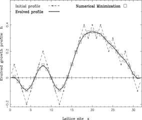
Figure 2: The initial and the evolved fields for a lattice composed of 32 sites. The approximate field evolution ($\square$) is calculated according to the relation (38) with a reduction of order $M=8$ (a) and $M=16$ (b) in the degrees of freedom. The field is plotted after 100 time steps using a temporal integration interval $\Delta t=1.0$. The fields were evolved using a diffusion parameter $\nu=0.01$.

Using the approximate evolution equation (38) together with a reduction operator ${\cal R}$ of order $M=8$ no difference occurs compared to the field evolution using all degrees of freedom. However for a reduction factor $\lambda=2$ as shown in figure 2 very small deviations can be observed.
We would like to point out, that both the exact calculation and the numerical results are highly dependent on linearity and adjointness of the Hamiltonian, which account physically for the existence of normal modes. A similar calculation for non-selfadjoint linear operators using singular value decomposition is given in the appendix.

5 A General Approach to Nonlinear Evolution Equations.

In this section we apply the theoretical concepts developed in section 2 and section 3 to the deterministic Kardar-Parisi-Zhang (KPZ) equation [7] and the deterministic Burgers equation [28]. Each equation provides a different type of non-linearity to the numerical minimization process and exhibits a different physical characteristics. As the main milestone in the direction of nonlinear surface growth the KPZ equation has been intensively investigated as the correct interface equation governing the physics of lateral growth phenomena [29]. The Burgers equation describes a vorticity-free compressible fluid flow and the velocity field ${\bf v}(x,t)$ becomes the analogue of the (surface) height function ${\bf h}(x,t)$ in the KPZ equation [30].
In this section we monitor the evolution of both fields ${\bf h}(x,t)$ and ${\bf v}(x,t)$ over different time scales. We compute the scaling characteristics for the field fluctuations and various observables are measured in the long time scaling regime. We compare the performance of the evolution using a reduced number of degrees of freedom with the evolution by direct numerical integration in time. In addition, by using transformations both equations can be mapped on the linear diffusion problem which was exactly solved regarding the reduction operator ${\cal R}$ in section 4. These transformations provide an alternative exact construction of the reduction operator ${\cal R}$ for both the KPZ and the Burgers equation.

5.1 The relevant degrees of freedom in the KPZ equation

The deterministic KPZ equation is defined as

$$\frac{\partial{\bf h}(x,t)}{\partial t}\;=\;\nu{\nabla}^{2}{\bf h}(x,t)+\kappa\big{[}\nabla{\bf h}(x,t)\big{]}^{2}\;,$$ (60)

where the first term on the right-hand side describes diffusive relaxation of the surface and the second term introduces the desired sideways growth. We discretize the linear part of equation (60) as proposed in (49) and the additional non-linear evolution operator defined in (2) as

$$Q_{i,j,k}\,:=\,\begin{cases}\quad\kappa/{\left({2\Delta t}\right)^{2}}&\;\mbox{if}\quad j=i-1;\,k=i-1\;\mbox{or}\;j=i+1;\,k=i+1\\ \,-\kappa/{\left({2\Delta t}\right)^{2}}&\;\mbox{if}\quad j=i-1;\,k=i+1\;\mbox{or}\;j=i+1;\,k=i-1\\ \qquad\;0&\;\mbox{else}\;.\end{cases}$$ (61)

In analogy to figure 1 in section 4 figure 3 shows the result of the short-time RG approach introduced in section 3.1 as applied to the initial surface profile.

   

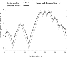
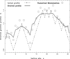
Figure 3: The initial and the evolved surface profiles for a lattice composed of 32 sites after 100 time steps (a) and 300 time steps (b) using a temporal integration interval $\Delta t=1$. The dashed curve represents the initial surface profile and the fields were evolved using a surface tension $\nu=0.01$ and a growth velocity $\kappa=0.1$.

The approximately evolved field displayed in figure 3 has been evolved according to a reduction of order $M=16$ in the degrees of freedom. Although the exact field evolution is recovered up to a time $t=100$, for $t=300$ the approximately evolved field exhibits a significant deviation from the evolution using all the degrees of freedom. For even larger times this results in uncontrollable numerical instabilities. The reported behaviour is expected for RG techniques which are not able to cope with scale interference [23].
To incorporate possible scale interference in the truncation procedure it is necessary to apply the concepts developed in section 3.2 and minimize $|{\cal E}|_{F}$ in (35). In addition to the direct numerical minimization procedure we further propose a more sophisticated approach based on the exact solution previously established in section 4. There it was shown that for the linear evolution problem ${\tilde{H}}=H$ the dynamic RSRG approach is equivalent to an exact diagonalization of the evolution operator. Since equation (60) can be mapped to the linear diffusion equation (48) using the Hopf-Cole transformation [7]

$${\bf w}(x,t)\;=\;e^{(\kappa/\nu)\cdot{\bf h}(x,t)}\;,$$ (62)

we are able to provide an exact reduction operator $R$ to evolve the field under a reduced number of degrees of freedom . In this case we decompose the construction of the reduction operator into three steps. First the initial field configuration ${\bf h}(x,0)$ is transformed to ${\bf w}(x,0)$ according to equation (62). The exactly calculated reduction operator including the relevant degrees of freedom of the linear evolution operator $H$ is applied within (38) to evolve the field in time. Using the inverse of transformation (62) the final field is recovered by using a reduced number of degrees of freedom.
In figure 4 the final evolved growth profile ${\bf h}$ after time $t=100$ is displayed for lattices of different size.

   

   

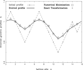
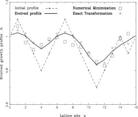
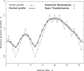
Figure 4: The initial and the evolved fields for a lattice composed of 16 sites ((a) and (b)) and 32 sites ((c) and (d)) after 100 time steps using a temporal integration interval $\Delta t=1.0$. The dashed curve represents the initial profile according to a periodic random initialization. The fields were evolved using a surface tension $\nu=0.01$ and a growth velocity $\kappa=0.1$.

The approximate field evolution is performed using a reduction operator calculated by direct numerical minimization ($square$) of $|{\cal E}|_{F}$ and alternatively using the exact transformation (62). Figure 4(a) shows the evolved growth profiles for a reduction factor of $\lambda=4/3$ for a periodic lattice composed of 16 sites, i.e. a truncation of order $M=4$. In figure 4(b) the initial field is equally evolved using a reduction factor $\lambda=2$. Compared to figure 4(a) the approximate equation (38) fails to evolve the field correctly. In Figure 4(c) and (d) the corresponding surface evolutions are displayed for a lattice composed of 32 lattice sites. The results displayed in figure 4 demonstrate that the construction of the reduction operator ${\cal R}$ is sensitive to finite size effects. In particular the reduction operator constructed by direct numerical minimization on a lattice composed of 16 sites fails to generate the characteristic paraboloid segments [7].
Analogously to the numerical minimization procedure of the linear diffusion problem carried out in section 4, the SQP minimization algorithm was provided by the NAG Library [27]. Again the optimal solution was found by the algorithm which in turn characterizes the minimization approach in (46) as a well defined and numerically stable procedure also in the non-linear case where no general analytical approach exists. However the numerical minimization turns out to be much more time consuming since the error operator norm $|{\cal E}|_{F}$ in equation (35) is increasingly complex for non-linear evolution problems.
To characterize the scaling behaviour of the KPZ equation we consider the decay of the density of surface steps for a lattice composed of $N$ sites, defined by

$$\rho(t)\;:=\;\frac{1}{N}\sum^{N}_{i=1}\left<{}\,\vrule\,{\nabla{\bf h}_{i}(t)}\,\vrule\,{}\right>\;.$$ (63)

Here the brackets $\left<{\;}\right>$ denote averaging with respect to an ensemble of initial surfaces ($t=0$) characterized by the covariance

$$\left<{}\,\vrule\,{{\bf h}_{i}-{\bf h}_{j}}\,\vrule\,{}\right>\;\sim\;|i-j|^{\zeta}$$ (64)

with the roughness exponent $\zeta$. The dynamic observable defined in equation (63) obeys the scaling relation [31]

$$\rho(t)\;\sim\;t^{(\zeta-1)/z}$$ (65)

where $z$ denotes the dynamic exponent for the lateral correlation length $\xi$ determined by $\xi\sim t^{1/z}$. For the deterministic KPZ equation a scaling relation for $z$ can be established in terms of $\zeta$ as [31]

$$z\;=\;2-\zeta\;.$$ (66)

To generate an ensemble of initial surfaces according to (64) we initialize the surface profile by the graph of a one dimensional Brownian bridge as visualized in figure 5.

Figure 5: An initial surface profile generated from the graph of a random walk using periodic boundary conditions (Brownian bridge).

The initial surface profile shown in figure 5 corresponds to a Brownian bridge of length $N$ introducing a finite size correction to the correlation function which vanishes for $N\longrightarrow\infty$. This dependence on the lattice size needs to be considered in a measurement for the roughness exponent of the theoretical value $\zeta=1/2$ [35]. According to the technical realization of the periodic boundary conditions the probability for the walker to go left and right after a certain number of surface steps depends on the remaining steps to go and the position of the walker.
In figure 6(a)-(d) the density of surface steps observable is compared for four different reduction factors $\lambda=4/3,8/5,2$ and $8/3$.

   

   

Figure 6: The inverse of the density of surface steps observable plotted according to the scaling relation $\,\rho(t)^{-1}\sim\sqrt[3]{t}\,$ for a different number of eliminated degrees of freedom ($\lambda=4/3,8/5,2$ and $8/3$). The observable is measured over a total time of 100 time evolution steps of temporal distance $\Delta t=1$ and the ensemble average was taken over 400 surfaces with $\zeta=1/2$. The surfaces were evolved using a surface tension $\nu=0.01$ and a growth velocity $\kappa=0.1$.

We expect a deviation from the exact scaling relation in the early time regime because of the finite size dependence of the initial surface profile constructed as a Brownian bridge. Therefore, inserting (66) into equation (65) we derive the scaling relation $\,\rho(t)^{-1}\sim t^{1/3}\,$ plotted in figure 6 valid in the long time regime. As expected both curves show a significant deviation from the theoretical scaling behaviour in the short time regime. For longer times the evolution generated by using a reduction operator providing more than half of all the degrees of freedom for the nonlinear surface growth process recovers the desired long-time linear behaviour. Using a reduction factor of $\lambda=2$ or an even higher order in the reduction of the degrees of freedom the observable measured using the approximate field evolution displays an increasing deviation from the measurement using a field evolved with all the degrees of freedom.
As a central observation in surface growth phenomena surface fluctuations exhibit a dynamical scaling behaviour [33]. The surface width of a growing surface is defined as [33]

$${\cal W}_{t}\;=\;\sqrt{\frac{1}{N}\sum^{N}_{i=1}\Big{(}{\bf h}_{i,t}-{\bar{h_{t}}}\Big{)}^{2}}\qquad\mbox{with}\quad{\bar{h_{t}}}\;=\;\frac{1}{N}\sum^{N}_{i=1}{\bf h}_{i,t}\;.$$ (67)

In particular the scaling of the interface width (67) on the length scale $N$ is expected to be of the form [29]

$${\cal W}_{t}\;=\;N^{\zeta}f_{t/N^{z}}\;,$$ (68)

where $f_{t/N^{z}}$ denotes a scaling function different from the one in the stochastic case. Using relation (66) we calculate for the KPZ equation the scaling characteristics

$$\frac{1}{\sqrt{N}}{\cal W}_{t}\;=\;f_{t/N^{3/2}}\;.$$ (69)

In figure 7 the surface width observable is plotted in analogy to figure 6 measured using equally evolved surface profiles.

   

   

Figure 7: The surface width observable plotted according to the scaling characteristics of the KPZ equation. From (a)-(d) increasing reduction factors of $\lambda=4/3$, $\lambda=8/5$, $\lambda=2$ and $\lambda=8/3$ are used. The observable is measured over a total time of 100 time evolution steps of temporal distance $\Delta t=1$. The ensemble average was taken over 400 surfaces with $\zeta=1/2$ each generated by a periodic random walk as displayed in figure 5. All surfaces were evolved using a surface tension $\nu=0.01$ and a growth velocity $\kappa=0.1$.

All measurements of the surface width observable are calculated according to an ensemble average of 400 surface configurations to be consistent with the literature [31]. The measurements for the observable ${\cal W}$ represent the same dependence on the reduction factor $\lambda$ as the analogue measurements for the observable $\rho$ in figure 6.

5.2 The relevant degrees of freedom in the Burgers equation

As a quasi one dimensional analogue of the Navier-Stokes equations the Burgers equation is defined as

$$\frac{\partial{\bf v}(x,t)}{\partial t}\;=\;\nu{\nabla}^{2}{\bf v}(x,t)\,-\,\kappa{\bf v}(x,t)\cdot\nabla{\bf v}(x,t)\;,$$ (70)

where the parameter $\nu$ denotes the viscosity of the velocity field ${\bf v}(x,t)$. The nonlinear term on the right hand side is a transport or convection term in which the speed of the convection depends on the magnitude of ${\bf v}(x,t)$ . Compared to the KPZ equation analyzed in the previous section the convection term provides a different discretization scheme to the direct numerical minimization procedure.
Inserting the transformation ${\bf v}(x,t)=(\partial/\partial x){\bf h}(x,t)$ into equation (70) we rederive the KPZ equation defined in (60). By further applying (62) results in the linear diffusion equation for which we can calculate the reduction operator exactly as described in section 4. Again, following the steps outlined for the case of the KPZ equation below (62) we are able to provide an alternative exact reduction operator ${\cal R}$ to evolve the velocity field under a reduced number of degrees of freedom.
Figure 8 shows an evolved velocity field after a total evolution time $t=100$ using a lattice composed of 32 sites.

   

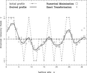
Figure 8: The initial and the evolved velocity fields for a lattice composed of 32 sites after 100 time steps using a temporal integration interval $\Delta t=1$. The initial velocity field configuration (dashed curve) is evolved with a reduction factor $\lambda=4/3$ (a) and $\lambda=2$ (b). The evolution using a reduced number of degrees of freedom is shown using a reduction operator constructed by numerical minimization and by using an exact transformation. The velocity fields were evolved with a surface tension $\nu=0.01$ and a growth velocity $\kappa=0.1$.

In figure 8 the performance between the reduction operator ${\cal R}$ constructed by directly minimizing $|{\cal E}|_{F}$ and the exact one using the proposed transformations is compared for two different reduction factors $\lambda=4/3$ and $\lambda=2$. Although both methods perform reasonably well for a reduction factor $\lambda=4/3$ for a reduction factor $\lambda=1/2$ the direct numerical minimization performs far superior to the evolution incorporating the exact transformations. The stated performance of the SQP algorithm using the NAG Library [27] is equal to the examined case of the KPZ equation in section 5.1, so that also in this case the numerical minimization converges in a well defined minimum subject to equation (35).
Burgers showed that the decay of the step density follows the dynamical scaling behaviour [28]

$$\mathinner{\langle{}|}{\bf v}(x,t)\mathinner{|{}\rangle}\;\sim\;t^{-\frac{1}{3}}$$ (71)

which is equivalent to the scaling relation (65) with $\zeta=1/2$ and $z=3/2$ using the transformation ${\bf v}(x,t)=(\partial/\partial x){\bf h}(x,t)$. Here the brackets $\left<{\;}\right>$ denote an ensemble average of stationary and locally uncorrelated initial velocity field configurations ${\bf v}(x,0)$. In figure 9 we have plotted the asymptotic time behaviour (71) over a total time $t=1000$.

   

Figure 9: The inverse of the decay of the density of surface steps observable plotted according to the scaling relation (71) for a reduction factor $\lambda=4/3$ (a) and $\lambda=2$ (b). The observable is measured over a total time of 1000 time evolution steps of temporal distance $\Delta t=1$. The ensemble average was taken over 400 random surfaces. All surfaces were evolved using a surface tension $\nu=0.01$ and a growth velocity $\kappa=0.1$.

The velocity field has been evolved by a reduction of order $M=8$ and $M=16$ degrees of freedom respectively, the latter corresponding to a $\lambda=2$ reduction. Following Burgers [28] we generated an ensemble of stationary and locally uncorrelated initial velocity field configurations ${\bf v}_{i}(x,0)$ by calculating

$${\bf v}_{i}(x,0)\;=\;(\partial/\partial x){\bf h}_{i}(x,0)\qquad\mbox{and}\quad i\in\{1,\dots,400\}\;.$$ (72)

In equation (72) ${\bf h}_{i}(x,0)$ denotes the graph of a Brownian bridge as shown in figure 5.
To confirm the results in figure 8 and 9 quantitatively we investigate the numerical stability within the evolution of the velocity field in dependence of the order of the truncation in the limit of long-time evolutionary dynamics. Using (38) together with an iterative construction of the reduction operator ${\cal R}^{M}$ of order $M$ according to equation (44), table 1 summarizes the mean square deviation (MSD) as measured in comparison with the exact velocity field evolution.

Table 1: The accuracy of the approximate velocity field evolution using direct numerical minimization as compared to the exact velocity field evolution using all degrees of freedom in the long-time limit. The approximate velocity field evolution is compared for a reduction of different orders by calculating the mean square deviation (MSD) between the approximately and the exactly evolved velocity field. All reductions calculated refer to an original lattice composed of 32 sites.

Reduction in the	Total evolution	Total evolution	Total evolution
degrees of freedom	time  $t=100$	time  $t=1000$	time  $t=10000$
of order $M=8$	$6.451\cdot 10^{-4}$	$7.906\cdot 10^{-5}$	$3.012\cdot 10^{-6}$
of order $M=12$	$1.866\cdot 10^{-3}$	$1.074\cdot 10^{-4}$	$5.737\cdot 10^{-6}$
of order $M=16$	$3.600\cdot 10^{-3}$	$1.534\cdot 10^{-4}$	$6.428\cdot 10^{-6}$
of order $M=20$	$8.852\cdot 10^{-3}$	$7.267\cdot 10^{-3}$	$9.851\cdot 10^{-4}$
of order $M=24$	$1.320\cdot 10^{-2}$	$8.976\cdot 10^{-3}$	$1.211\cdot 10^{-3}$
of order $M=28$	$2.319\cdot 10^{-2}$	$1.258\cdot 10^{-2}$	$1.473\cdot 10^{-3}$

The convergence in time of the MSD for each order of the reduction in the degrees of freedom illustrates the numerical stability in the long-time scaling regime. However, for a reduction factor $\lambda>2$ ($M=16$) the accuracy of the approximately evolved velocity field in the long-time evolution decreases by at least two orders of magnitude. This indicates that at least half of the available degrees of freedom are relevant for an accurate evaluation of the long-time characteristics in the Burgers equation.

6 Conclusions

In this paper we applied an operator real-space RG method to partial differential equations (PDEs) in general. The fundamental concept is to construct a linear map, the reduction operator ${\cal R}$, projecting to a subspace of the full vector space including the relevant degrees of freedom governing the physics of the evolutionary dynamics. In technical terms the reduction operator is composed as the product of the truncation and embedding operator, which are already established objects in the equilibrium real-space RG literature.
Two basic approaches are provided for the construction of the reduction operator ${\cal R}$. In the first approach a transformation to a linear PDE is used for which the reduction operator can be constructed using exact or numerically fast diagonalization techniques. If such a transformation is missing a direct numerical minimization is applied using a sequential quadratic programming (SQP) algorithm to construct the reduction operator. The advantage of the first approach over the second one is dominated by the saving of computer time depending on the particular nonlinear problem of interest. However, again depended on the particular PDE, it was observed in this work that numerical instabilities in the field evolution can prove the first approach to be useless. Although the computer calculation time increases with the lattice size the computed reduction operator does not depend on a particular initial field configuration and can be stored and applied to the evolution of any other initial field configuration.
In fully developed turbulence or related non-integrable dynamical systems the dynamics and evolution of many degrees of freedom interacts through nonlinear PDEs. Direct numerical simulations are difficult and show a clear demand for a reduction to the relevant degrees of freedom. Choosing the Burgers equation to test our RG approach we have examined one of the simplest archetypes describing a vorticity-free, compressible fluid flow. The measured decay of the step density can be generalized to higher order correlation functions corresponding to structure functions in fully developed turbulence [30].
One of the goals of the real-space RG method presented in this paper is certainly the reduction in complexity of the problem yielding to a reduced amount of computer time within simulations, after a reduction operator ${\cal R}$ has been provided. Since this operator contains information on the relevant degrees of freedom the proposed real-space RG method gives rise to improved understanding of the physics of non-linear evolutionary dynamics.

Acknowledgment

The authors wish to thank the Department of Mathematical Physics at the University of Bielefeld, Germany, for the warm and kind atmosphere during their visit in which the foundations of this work were developed. Special thanks are given to Silvia N. Santalla for her continuous help in the realization of the project.

Appendix

In the case of a non-selfadjoint Hamiltonian, the approach in section 4 must be slightly changed. There exists no decomposition of the functional space into eigenvectors of the evolution operator $H$, so the natural approach requires a singular value decomposition [25]

$$H\;=\;\sum_{i=1}^{N}E_{i}\mathinner{|{u_{i}}\rangle}\mathinner{\langle{v_{i}}|}\;.$$ (73)

In equation (73) the vectors $\{\mathinner{|{v_{i}}\rangle}\}_{i}$ denote the “input states” and the vectors $\{\mathinner{|{u_{i}}\rangle}\}_{i}$ make up the “output states”. It is important to state that both sets of vectors belong to the same functional space.
Changing slightly our notation for clarity $\mathinner{|{\phi}\rangle}$ denotes the target state, whose removal minimizes the error operator

$${\cal E}\;:=\;{\cal P}_{\mathinner{|{\phi}\rangle}}+\Delta t\left[H{\cal P}_{\mathinner{|{\phi}\rangle}}+{\cal P}_{\mathinner{|{\phi}\rangle}}H-\mathinner{\langle{\phi}|}H\mathinner{|{\phi}\rangle}{\cal P}_{\mathinner{|{\phi}\rangle}}\right]\;.$$ (74)

We decompose $\mathinner{|{\phi}\rangle}$ in both the input and the output basis as

$$\mathinner{|{\phi}\rangle}\;=\;\sum_{i=1}^{N}\mu_{i}\mathinner{|{v_{i}}\rangle}\qquad\mbox{and}\qquad\mathinner{|{\phi}\rangle}\;=\;\sum_{i=1}^{N}\chi_{i}\mathinner{|{u_{i}}\rangle}\;\;.$$ (75)

Analogously to (4) we arrange the resulting operators in (74) using the two alternative representations in (75) by

$${\cal P}_{\mathinner{|{\phi}\rangle}} \;=\;\sum_{i,j=1}^{N}\chi_{i}\mu_{j}\mathinner{|{u_{i}}\rangle}\mathinner{\langle{v_{j}}|}\qquad\quad\mathinner{\langle{\phi}|}H\mathinner{|{\phi}\rangle}\;=\;\sum_{i=1}^{N}\mu_{i}\chi_{i}E_{i}\;\equiv\;\mathinner{\langle{H}\rangle}$$

$$H{\cal P}_{\mathinner{|{\phi}\rangle}} \;=\;\sum_{i,j=1}^{N}E_{i}\mu_{i}\mu_{j}\mathinner{|{u_{i}}\rangle}\mathinner{\langle{v_{j}}|}\qquad\quad{\cal P}_{\mathinner{|{\phi}\rangle}}H\;=\;\sum_{i,j=1}^{N}\chi_{i}\chi_{j}E_{j}\mathinner{|{u_{i}}\rangle}\mathinner{\langle{v_{j}}|}\quad.$$ (76)

Therefore, in the basis of the evolution operator

$${\cal E} \;=\;\sum_{i,j=1}^{N}{\cal E}_{ij}\mathinner{|{u_{i}}\rangle}\mathinner{\langle{v_{j}}|}$$

$$\quad\mbox{with}\qquad{\cal E}_{ij}\;=\;\chi_{i}\mu_{j} +\Delta t\Big{(}E_{i}\mu_{i}\mu_{j}+\chi_{i}\chi_{j}E_{j}-\mathinner{\langle{H}\rangle}\chi_{i}\mu_{j}\Big{)}\;.$$ (77)

Squaring and retaining only terms which are linear in $\Delta t$

$${\cal E}_{ij}^{2}\;\approx\;\chi_{i}^{2}\mu_{i}^{2}+2\Delta t\Big{(}E_{i}\mu_{i}\chi_{i}\mu_{j}^{2}+E_{j}\chi_{i}^{2}\chi_{j}\mu_{j}-\mathinner{\langle{H}\rangle}\chi_{i}^{2}\mu_{j}^{2}\Big{)}\;.$$ (78)

Summation over all the values in (78) yields

$$\sum_{i,j=1}^{N}{\cal E}_{ij}^{2}\;=\;1\,+\,2\cdot\Delta t\mathinner{\langle{H}\rangle}$$ (79)

to first order in $\Delta t$. The result is equivalent to equation (56) and a again $\mathinner{\langle{H}\rangle}$ must be minimized. However one has to remember that the set of numbers $\{\mu_{i}\}_{i}$ and $\{\chi_{i}\}_{i}$ are not independent since they represent the same field.
The idea is to represent the vectors $\{\mathinner{|{v_{i}}\rangle}\}_{i}$ in the basis of the vectors $\{\mathinner{|{u_{i}}\rangle}\}_{i}$ according to

$$\mathinner{|{v_{i}}\rangle}\;=\;\sum_{j=1}^{N}C_{ij}\mathinner{|{u_{j}}\rangle}$$ (80)

The matrix $C_{ij}$ may be obtained by the SVD of the evolution operator $H$ using

$$C_{ij}\;\equiv\;\mathinner{|{v_{j}}\rangle}\mathinner{\langle{u_{i}}|}\;.$$ (81)

The equality of both representations in (75) yields a relation between the $\{\mu_{i}\}_{i}$ and the $\{\chi_{i}\}_{i}$:

$$\sum_{i=1}^{N}\mu_{i}\mathinner{|{v_{i}}\rangle}\,=\,\sum_{i,j=1}^{N}\mu_{i}C_{ij}\mathinner{|{u_{j}}\rangle}\,=\,\sum_{j=1}^{N}\left(\sum_{i=1}^{N}C_{ij}\mu_{i}\right)\mathinner{|{u_{j}}\rangle}\;=\;\sum_{j=1}^{N}\chi_{j}\mathinner{|{u_{j}}\rangle}$$ (82)

As the $\{\mathinner{|{u_{j}}\rangle}\}_{i}$ form an orthonormal basis we may deduce

$$\chi_{j}\;=\;\sum_{i=1}^{N}C_{ij}\mu_{i}\;.$$ (83)

Using (6) and inserting (83) the value to be minimized equals

$$\mathinner{\langle{H}\rangle}\;=\;\mathinner{\langle{\phi}|}H\mathinner{|{\phi}\rangle}\;=\;\sum_{i=1}^{N}\mu_{i}\chi_{i}E_{i}\;=\;\sum_{i,j=1}^{N}E_{i}\mu_{i}C_{ji}\mu_{j}\;\;.$$ (84)

Equation (84) defines a quadratic form based on a matrix which is not symmetric. Defining

$$K_{ij}\equiv\frac{1}{2}\left(E_{i}C_{ji}+E_{j}C_{ij}\right)$$ (85)

the problem is reduced to the minimization of the quadratic form

$$\mathinner{\langle{H}\rangle}=\sum_{i,j=1}^{N}K_{ij}\mu_{i}\mu_{j}$$ (86)

with the restriction $\sum_{i}\mu_{i}^{2}=1$. This problem is equivalent to the self-adjoint case examined in section 4 and the solution is the lowest eigenvalue of the matrix $K$.
The eigenvector corresponding to the minimum eigenvalue of the matrix $K$ is to be interpreted as a set of $\mu_{i}$ values. Thus, the $\mathinner{|{\phi}\rangle}$ eigenvector shall be given by the calculation of $\sum_{i}\mu_{i}\mathinner{|{u_{i}}\rangle}$ with the appropriate values of $\mu_{i}$.

References

- [1] L.P. Kadanoff. Physics 2, 263 (1966).
- [2] K.G. Wilson. Phys. Rev. B4, 3174 (1971). Phys. Rev. B4, 3184 (1971). Phys. Rev. Lett. 28, 548 (1972).
- [3] K.G. Wilson. Rev. Mod. Phys. 47, 773 (1975).
- [4] S.K. Ma. Modern Theory of Critical Phenomena. Benjamin/Cummings Publishing Company, Reading (1976).
- [5] P.C. Hohenberg and B.I. Halperin Rev. Mod. Phys. 49, 435 (1977).
- [6] D. Forster, D. Nelson and M. Stephen Phys. Rev. A 16, 732 (1977).
- [7] M. Kardar, G. Parisi and Y.-C. Zhang Phys. Rev. Lett. 56, 889 (1986).
- [8] E. Medina, T. Hwa, M. Kardar and Y. Zhang Phys. Rev. A 39, 3053 (1989).
- [9] E. Frey and U.C. Taeuber Phys. Rev. E 50, 1024 (1994).
- [10] T. Nattermann and L.H. Tang Phys. Rev. A 45, 7156 (1992).
- [11] J.P. Bouchaud and M.E. Cates Phys. Rev. E 47, R1455 (1993).
- [12] M. Schwartz and S.F. Edwards Europhys. Lett. 20, 301 (1992).
- [13] T. Halpin-Healy Phys. Rev. Lett. 62, 442 (1990). Phys. Rev. A 42, 711 (1990).
- [14] D.E. Wolf and J. Kertsz Europhys. Lett. 4, 651 (1987).
- [15] B.M. Forrest and L. Tang J. Stat. Phys. 60, 181 (1990).
- [16] M. Beccaria and G. Curci Phys. Rev. E, 4560 (1994).
- [17] S.R. White. Phys. Rev. B48, 10345 (1993).
- [18] J.R. de Sousa. Phys. Lett. A216, 321 (1996).
- [19] M.A. Martin-Delgado, J. Rodríguez-Laguna and G. Sierra Nucl. Phys. B473, 685 (1996).
- [20] A. Degenhard. J. Phys. A: Math. Gen. 33, 6173 (2000).
- [21] J. Gonzales, M.A. Martin-Delgado, G. Sierra and A.H. Vozmediano New and old real-space renormalization group methods. In: Quantum Electron Liquids and High- Superconductivity. Lecture Notes in Physics 38, Springer, Berlin (1995).
- [22] N. Goldenfeld, A. McKane and Q. Hou. J. Stat. Phys. 93, 699 (1998).
- [23] Q. Hou, N. Goldenfeld and A. McKane. Phys. Rev. E 63, 36125 (2001).
- [24] A. Degenhard and J. Rodríguez-Laguna. cond-mat/0106155 (2001). Submitted to Phys. Rev. E.
- [25] W.H. Press, S.A. Teukolsky, W.T. Vetterling and B.P. Flannery. Numerical Recipies. The Art of Scientific Computing. Cambridge, University Press (1992).
- [26] P.E. Gill, W. Murray and M.H. Wright. Practical optimization. New York, Academic Press (1981).
- [27] The Numerical Algorithms Group Inc. NAG Fortran Library, Mark 17. Oxford, United Kingdom (1995).
- [28] J.M. Burgers. The Nonlinear Diffusion Equation. Riedel, Boston (1974).
- [29] T. Halpin-Healy and Y.-C. Zhang. Phys. Rep. 254, 215 (1995).
- [30] J. Krug. Phys. Rev. Lett. 72(18), 2907 (1994).
- [31] J. Krug and H. Spohn. Phys. Rev. A 38(8), 4271 (1988).
- [32] S.E. Esipov and T.J. Newman. Phys. Rev. E 48(6), 1046 (1993).
- [33] J.G. Amar and F. Family. Phys. Rev. E 47(3), 1595 (1993).
- [34] Y. Kuramoto. Chemical Oscillations, Waves and Turbulence. Springer, Berlin (1984).
- [35] C. Itzykson and J.M. Drouffe. Statistical field theory. University Press, Cambridge (1991).