Hidden symmetry and knot solitons in a charged two-condensate Bose system

Abstract

We show that a charged two-condensate Ginzburg-Landau model or equivalently a Gross-Pitaevskii functional for two charged Bose condensates, can be mapped onto a version of the nonlinear $O(3)$ $\sigma$-model. This implies in particular that such a system possesses a hidden $O(3)$ symmetry and allows for the formation of stable knotted solitons.

For over forty years there has been a wide interest in condensed matter systems with several coexisting Bose condensates [1]. Here we shall investigate the physically important example of two charged condensates together with their electromagnetic interaction. This system is described by a Ginzburg-Landau model with two flavors of Cooper pairs. Alternatively, it relates to a Gross-Pitaevskii functional with two charged condensates of tightly bound fermion pairs, or some other charged bosonic fields. Such theoretical models have a wide range of applications and have been previously considered in connection of two-band superconductivity. Indeed, these models describe superconductivity in transition metals [1, 2]. The presence of two condensates has been observed in experiments on $Nb$, $Ta$ and $V$ as well as in $Nb$-doped $SrTiO_{3}$ [3]. More recently the renewed interest to two-gap superconductivity was sparked by discovery of the the two-band superconductor with surprisingly high critical temperature $MgB_{2}$ [4]. It has also been argued in [5] that under certain conditions liquid metallic hydrogen might allow for the coexistence of superconductivity with both electronic and protonic Cooper pairs. In a liquid metallic deuterium a deuteron superfluidity may similarly coexist with superconductivity of electronic Cooper pairs [6] (see also [7]).

Here we shall be particularly interested in an exact equivalence between the two-flavor Ginzburg-Landau-Gross-Pitaevskii (GLGP) model and a version of the nonlinear O(3) $\sigma$-model introduced in [8]. We expose this equivalence by presenting an exact, explicit change of variables between the two models. The model in [8] is particularly interesting since it describes topological excitations in the form of stable, finite length knotted closed vortices [9]. The equivalence then implies that a system with two charged condensates similarly supports topologically nontrivial, knotted solitons. Previously it has been argued that these topological defects could play an important role in high energy physics [8]-[13]. The purpose of the present Letter is to discuss the condensed matter counterparts.

A system with two electromagnetically coupled, oppositely charged Bose condensates can be described by a two-flavour (denoted by $\alpha=1,2$) Ginzburg-Landau or Gross-Pitaevskii (GLGP) functional,

$$F=\int d^{3}x\ \biggl{[}\frac{1}{2m_{1}}\left|\left(\hbar\partial_{k}+i\frac{2e}{c}A_{k}\right)\Psi_{1}\right|^{2}+$$ (1)

$$\frac{1}{2m_{2}}\left|\left(\hbar\partial_{k}-i\frac{2e}{c}A_{k}\right)\Psi_{2}\right|^{2}+{V}(|\Psi_{1,2}|^{2})+\frac{{\bf B}^{2}}{8\pi},\biggr{]}$$ (2)

where we take

$\displaystyle{V}(|\Psi_{1,2}|^{2})=-b_{\alpha}|\Psi_{\alpha}|^{2}+\frac{c_{\alpha}}{2}|\Psi_{\alpha}|^{4}$

Here we shall consider the general case where the two condensates are characterized by different effective masses $m_{\alpha}$, different coherence lengths $\xi_{\alpha}=\hbar/\sqrt{2m_{\alpha}b_{\alpha}}$ and different concentrations $N_{\alpha}=<|\Psi_{\alpha}|^{2}>={b_{\alpha}}/{c_{\alpha}}$ [14]. The properties of the corresponding model with a single charged Bose field are well known. In that case the field degrees of freedom are the massive modulus of the single complex order parameter and a vector field which gains a mass due to the Meissner-Higgs effect. The important property of the present GLGP model is that the two charged fields are not independent but there is a nontrival coupling which is mediated by the electromagnetic field. This implies that we have a nontrivial, hidden topology which becomes obscured when we represent the model in the variables (2). In order to expose the topological structure we introduce a new set variables, involving a massive field $\rho$ which is related to the densities of the Cooper pairs and a three-component unit vector field ${\bf\vec{n}}$. The important feature of these new variables is their gauge invariance: Neither the relative phase of the condensates $\Psi_{1}$ and $\Psi_{2}$ nor the gauge field $\bf A$ enters in the free energy functional when represented in these new variables.

We start by introducing variables $\rho$ and $\chi_{1,2}$ by

$\displaystyle\Psi_{\alpha}={\sqrt{2m_{\alpha}}}\ \rho\chi_{\alpha}$

where the complex $\chi_{\alpha}=|\chi_{\alpha}|e^{i\varphi_{\alpha}}$ are chosen so that $|\chi_{1}|^{2}+|\chi_{2}|^{2}=1$. The modulus $\rho$ then has the following expression:

$\displaystyle\rho^{2}=\frac{1}{2}\left(\frac{|\Psi_{1}|^{2}}{m_{1}}+\frac{|\Psi_{2}|^{2}}{m_{2}}\right)$

In terms of the variables $\rho$ and $\chi_{\alpha}$ the free energy density in (2) reads as follows:

$$F = \hbar^{2}(\partial\rho)^{2}+\hbar^{2}\rho^{2}|(\partial_{k}+i{\tilde{A}}_{k})\chi_{1}|^{2}+$$ (4)

$$\hbar^{2}\rho^{2}|(\partial_{k}-i{\tilde{A}}_{k})\chi_{2}|^{2}+\frac{{\bf B}^{2}}{8\pi}+{V}$$

where we denote ${\tilde{A}}_{k}=\frac{2e}{\hbar c}A_{k}$, and $\partial$ (without an index) is the ordinary $\nabla$ operator. The standard gauge invariant expression for the supercurrent density

$${\bf J} = \frac{i\hbar e}{m_{1}}\left\{\Psi_{1}^{*}\partial\Psi_{1}-\Psi_{1}\partial\Psi_{1}^{*}\right\}-\frac{i\hbar e}{m_{2}}\left\{\Psi_{2}^{*}\partial\Psi_{2}-\Psi_{2}\partial\Psi_{2}^{*}\right\}$$ (5)

$$- \frac{4e^{2}}{c}\left(\frac{|\Psi_{1}|^{2}}{m_{1}}+\frac{|\Psi_{2}|^{2}}{m_{2}}\right){\bf A}$$ (6)

becomes in these new variables

$${\bf J}=4\hbar e\rho^{2}\left[\frac{\bf j}{2}-{\bf{\tilde{A}}}\right].$$ (7)

where

$\displaystyle{\bf j}=i[\chi_{1}\partial\chi_{1}^{*}-\chi_{1}^{*}\partial\chi_{1}-\chi_{2}\partial\chi_{2}^{*}+\chi_{2}^{*}\partial\chi_{2}].$

We introduce a gauge-invariant vector field $\vec{\sf C}$, directly related to the supercurrent density by

$$\vec{\sf C}=\frac{{\bf J}}{e\rho^{2}}$$ (8)

We then rearrange the terms in (4) as follows: We add and subtract from (4) a term $\frac{1}{4}\hbar^{2}\rho^{2}{\bf j}^{2}$ and observe that the following expression

$$\hbar^{2}\rho^{2}\left[|\partial\chi_{1}|^{2}+|\partial\chi_{2}|^{2}-\frac{{\bf j}^{2}}{4}\right]$$ (9)

is also gauge invariant. Indeed if we introduce the gauge invariant field

$${\bf\vec{n}}=({\bar{\chi}}\ ,\ {\vec{\sigma}}\ \chi),$$ (10)

where $\chi=(\chi_{1},{\chi_{2}^{*}})$ and $\vec{\sigma}$ are the Pauli matrices, then ${\bf\vec{n}}$ is a unit vector $|{\bf\vec{n}}|=1$ and we can write (9) as follows,

$$\hbar^{2}\rho^{2}\left[|\partial\chi_{1}|^{2}+|\partial\chi_{2}|^{2}-\frac{{\bf j}^{2}}{4}\right]=\frac{1}{4}\hbar^{2}\rho^{2}(\partial{\bf\vec{n}})^{2}$$ (11)

Consider now the remaining terms in (2). For the magnetic field we get

$${\bf B}={\rm rot}{\bf A}=-\frac{c}{8e}{\rm rot}\vec{\sf C}+\frac{\hbar c}{4e}{\rm rot}{\bf j}$$ (12)

where ${\rm rot}\ \bf j$ can be written in terms of the unit vector ${\bf\vec{n}}$ as follows:

$\displaystyle{\rm rot}{\bf j}=\frac{1}{2}{\bf\vec{n}}\cdot\partial_{i}{\bf\vec{n}}\times\partial_{j}{\bf\vec{n}}$

Combining these we then arrive at our main result: The GLGP free energy density becomes

$$F = \frac{\hbar^{2}\rho^{2}}{4}(\partial{\bf\vec{n}})^{2}+\hbar^{2}(\partial\rho)^{2}+$$ (15)

$$\frac{\hbar^{2}c^{2}}{512\pi e^{2}}\left(\frac{1}{\hbar}[\partial_{i}{\sf C}_{j}-\partial_{j}{\sf C}_{i}]-{\bf\vec{n}}\cdot\partial_{i}{\bf\vec{n}}\times\partial_{j}{\bf\vec{n}}\right)^{2}$$

$$+\frac{\rho^{2}}{16}\vec{\sf C}^{2}+{{V}}(\rho,n_{3})$$

where we identify a version of the nonlinear O(3) $\sigma$-model introduced in [8]

$$F_{0}\ =\ \frac{\hbar^{2}\rho^{2}}{4}(\partial{\bf\vec{n}})^{2}+\frac{\hbar^{2}c^{2}}{512\pi e^{2}}\left({\bf\vec{n}}\cdot\partial_{i}{\bf\vec{n}}\times\partial_{j}{\bf\vec{n}}\right)^{2}$$ (16)

in interaction with a vector field $\vec{\sf C}$. With this we have completed the mapping between the two-condensate GLGP model (2) and (15), which is an extension of the model (16) introduced in [8]. We emphasize that this involves an exact change of variables between the GLGP model and (15). This change of variables in particular eliminates the gauge field and as a consequence the final result involves only the physically relevant field degrees of freedom that are present in the two-condensate system.

Note in particular the appearance of the mass for $\vec{\sf C}^{2}$ which is a manifestation of the Meissner effect; the London magnetic field penetration length is $\lambda^{2}=\frac{c^{2}}{16\pi e^{2}}\left[\frac{|\Psi_{1}|^{2}}{m_{1}}+\frac{|\Psi_{2}|^{2}}{m_{2}}\right]^{-1}=\frac{c^{2}}{32\pi e^{2}\rho^{2}}$. We also emphasize that the contribution ${\bf\vec{n}}\cdot\partial_{i}{\bf\vec{n}}\times\partial_{j}{\bf\vec{n}}$ to the magnetic field term in (15), (16) is a fundamentally important property of the two-condensate system which has no counterpart in a single condensate system. Indeed, it is exactly due to the presence of this term that the two-condensate system acquires properties which are qualitatively very different from those of a single-condensate system: This term describes the magnetic field that becomes induced in the system due to a nontrivial electromagnetic interaction between the two condensates.

The potential term ${V}$ depends only on Cooper pair concentrations and masses, and it is a function of the modulus $\rho$ and the $n_{3}$ component of the vector ${\bf\vec{n}}$ only. In particular, we can write the mass term in (15) explicitely as follows:

$${V} = A+Bn_{3}+Cn_{3}^{2}.$$ (17)

Where

$$A = \rho^{2}[4c_{1}m_{1}^{2}+4c_{2}m_{2}^{2}-b_{1}m_{1}-b_{2}m_{2}]$$ (18)

$$B = \rho^{2}[8c_{2}m_{2}^{2}-8c_{1}m_{1}^{2}-b_{2}m_{2}+b_{1}m_{1}]$$ (19)

$$C = 4\rho^{2}[c_{1}m_{1}^{2}+c_{2}m_{2}^{2}]$$ (20)

This mass term determines the energetically preferred ground state value for $n_{3}$, which we denote by ${\tilde{n}_{3}}$. Explicitely,

$${\tilde{n}_{3}}=\frac{\frac{N_{1}}{m_{1}}-\frac{N_{2}}{m_{2}}}{\frac{N_{1}}{m_{1}}+\frac{N_{2}}{m_{2}}}$$ (21)

Thus the ground state value of ${\bf\vec{n}}$ is a circle specified by the condition $n_{3}={\tilde{n}}_{3}$ on the unit two-sphere. This yields a uniform, unperturbed ground state for the condensates. Note that the ground state value only depends on the concentrations $N_{\alpha}$ and the masses $m_{\alpha}$ of the Cooper pairs.

However, here we are mostly interested in topological defects where the unit vector ${\bf\vec{n}}$ locally deviates from this ground state value. This then corresponds to the formation of a local inhomogeneity in the densities of the Cooper pairs. But in order to ensure a finite energy, at a certain distance from the inhomogeneity the vector ${\bf\vec{n}}$ should return to the circle defined by (21).

Indeed, the equivalence between the models (2) and (15) reveals a hidden topological structure in (2) which has a number of important physical consequences. In particular, it leads to the understanding of vortex types which are allowed by a two-condensate system: The model (16) is known to admit topological defects that have the shape of stable knotted solitons and are characterized by a nontrivial Hopf invariant [8]-[12], (see also comment [15]). The simplest nontrivial solution to the equations of motion that follow from (16) was proposed in [8]. In terms of vector ${\bf\vec{n}}$ it forms a toroidal vortex ring, twisted once around its core before joining the ends. The equivalence between the two-condensate model (2) and (15) then implies that the GLGP model with two charged condensates not only possesses a hidden $O(3)$ symmetry, but should also allow for the formation of such knotted vortex solitons. The stability of these topological defects has been confirmed in extensive numerical simulations [9]-[12] (for video animation of the numerical simulations of the knotted solitons see the www-address indicated in Ref. [12]). Indeed, the knotted vortex solitons e.g. in a two-condensate superconductor should consist of finite-length stable closed vortices, which carry a nontrivial helical configuration of the magnetic field. These finite length closed vortices have properties which are substantially different from those of a loop which is formed by an ordinary Abrikosov vortex. In particular: the present vortices are protected against shrinkage by the third term in (15) [second term in (16)].

Since the variable $n_{3}$ acquires the preferable value (21) in the ground state, the knotted solitons have the following form: At spatial infinity the unit vector ${\bf\vec{n}}$ assumes a value on the circle which is defined by the condition $n_{3}={\tilde{n}_{3}}$. We denote this value of ${\bf\vec{n}}$ at spatial infinity by

$${\bf\vec{n}}^{\infty}=(n_{1}^{\infty},n_{2}^{\infty},{\tilde{n}_{3}})\ \ \ \ \ \ \ ({\bf\vec{n}}^{\infty}={\bf\vec{n}}({\bf x}\rightarrow\infty)).$$ (22)

At the center of a knotted soliton the unit vector then reaches a value which corresponds to the opposite point on the unit sphere. In the case of a nontrivial knotted soliton the curve where the vector ${\bf\vec{n}}$ coincides with this opposite point value in general forms a closed loop or a knot. This is the core of the knotted soliton and we denote it by [18]

$${\bf\vec{n}}_{0}=(-n_{1}^{\infty},-n_{2}^{\infty},-{\tilde{n}_{3}})\ \ \ \ \ \ ({\bf\vec{n}}{\rm\ value\ at\ core})$$ (23)

At the core the densities of the condensates are characterized by the following non-vanishing values $|\Psi_{1}({\bf\vec{n}}_{0})|^{2}=\frac{m_{1}}{m_{2}}N_{2};\ \ |\Psi_{2}({\bf\vec{n}}_{0})|^{2}=\frac{m_{2}}{m_{1}}N_{1}$. In between the core where ${\bf\vec{n}}={\bf\vec{n}}_{0}$ and the boundary where ${\bf\vec{n}}\to{\bf\vec{n}}^{\infty}$ the unit vector ${\bf\vec{n}}$ in general rotates in a manner which is determined by the ensuing Hopf invariant [19]. Consequently a knotted solitons can be characterized by the number of rotations which are performed by the component of ${\bf\vec{n}}$, which is perpendicular to the axis defined by the boundary conditions ${\bf\vec{n}}^{\infty}$ and ${\bf\vec{n}}_{0}$ when we move around the knotted soliton by covering it once in toroidal and once in poloidal directions over any surface which is located between the core ${\bf\vec{n}}={\bf\vec{n}}_{0}$ and the boundary ${\bf\vec{n}}={\bf\vec{n}}^{\infty}$. In particular, in the region between the core and the boundary the magnetic field acquires a contribution from ${\bf\vec{n}}$ with a helical geometry, ${\bf B}^{h}\propto{\bf\vec{n}}\cdot\partial_{i}{\bf\vec{n}}\times\partial_{j}{\bf\vec{n}}$.

A schematic plot of a toroidal-shaped knot soliton is given on Fig. 1.

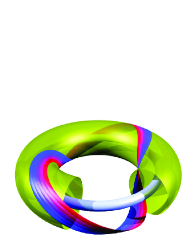
FIG. 1.: A schematic plot illustrating helical geometry of the vector ${\bf\vec{n}}$ in a simplest toroidal knot soliton (for simplicity we neglected anisotropy effects connected with nonzero mass of the $n_{3}$ component of the vector ${\bf\vec{n}}$). The toroidal hollow surface is a surface situated between the knot core ${\bf\vec{n}}_{0}$ and the knot boundary ${\bf\vec{n}}^{\infty}$. On this surface the vector ${\bf\vec{n}}$ has a constant projection to the axis defined by the boundary conditions ${\bf\vec{n}}^{\infty}$ and ${\bf\vec{n}}$. The spiral lines on this surface indicate the lines where the vector ${\bf\vec{n}}$ has some particular constant position on the unit sphere (the picture schematically shows a toroidal knot soliton which, in terms of the vector ${\bf\vec{n}}$, was twisted twice around its core before joining its ends). If we proceed along an arbitrary path over this surface covering the knot soliton once in toroidal direction and then once in poloidal direction, the vector ${\bf\vec{n}}$ will perform $n$ and $m$ rotations correspondingly, according to the Hopf invariant which characterizes the given soliton. In a general case the fluxtube can also be knotted (see also animations available at http address [9] ).

Finally we comment on the length scales that are present in our system. For simplicity we assume that the two condensates have equal coherence lengths $\xi_{1}=\xi_{2}=\xi$. In this case one concludes immediately that (15) has two different length scales. These are $\lambda$ which is the mass of the field $\vec{\sf C}$, and $\xi$ which is the mass of the component $n_{3}$ and relates to the coherence lengths of condensates. In the type-I limit which corresponds to $\lambda<<\xi$, and in the type-II limit where $\lambda>>\xi$ the characteristic sizes of knotted solitons are then determined by different factors: In the type-I limit the size is determined by an interplay of the terms $(\partial{\bf\vec{n}})^{2}$ and $({\bf\vec{n}}\cdot\partial_{i}{\bf\vec{n}}\times\partial_{j}{\bf\vec{n}})^{2}$ which implies that the size is of order $\lambda$ [20]. In the type II limit the size of the soliton is determined by the large mass of $n_{3}$ and thus it is of order of $\sqrt{\lambda\xi}$.

In conclusion, we have argued that charged two-condensate Bose systems possess a number of interesting properties which are qualitatively different from those of a single condensate system. In particular they can support stable knotted solitons as topological defects. Indeed, we find it remarkable that a GLGP functional for a two-component charged superfluid becomes intimately related to the model introduced by one of the authors in [8] which has been previously found to be relevant for strong interaction physics [9, 10]. This is a manifestation of the universal character of the model, which appears to describe a wide range of systems despite the differences in their physical origins. As a consequence the possibility of experimental investigation of the formation, properties and interactions of knotted solitons in approproate superfluids ( e.g. $MgB_{2}$, $Nb$, $Ta$, $V$ , $Nb$-doped $SrTiO_{3}$) along with numerical simulations, could then shed light even on the properties of similar objects in nonabelian gauge theories of fundamental interactions.

E.B. gratefully acknowledges numerous fruitful discussions with Prof. G. E. Volovik, and Prof. N.W. Ashcroft, Dr. V. Cheianov, Prof. S. Girvin and Prof. A.J. Leggett for useful comments. L.F. thanks L.P. Pitaevskii for discussions and the Department for Theoretical Physics of the Uppsala University for hospitality. A.N. thanks Helsinki Institute of Physics for hospitality during the completion of this work. We also thank M. Lübcke for plotting the figure. E.B. has been supported by grant STINT IG2001-062 and the Swedish Royal Academy of Science. L.F. has been supported by grants RFFR 99-0100101, INTAS 99-01705 and CRDF grant RM1-2244.

REFERENCES

- [1] H. Suhl, B.T. Matthias, L.R. Walker, Phys.Rev.Lett.3, 552 (1959)
- [2] J. Kondo Progr. Teor. Phys. 29 1 (1963); D.R. Tilley Proc. Royal Phys. Soc 84 573 (1964); A.J. Leggett, Prog. of Theor.Phys. 36, 901 (1966)
- [3] see e.g. L. Shen, N.Senozan, N. Phillips Phys. Rev. Lett. 14 1025 (1965); G. Binnig, A. Baratoff, H. E. Hoenig, J. G. Bednorz Phys. Rev. Lett. 45, 1352 (1980)
- [4] see e.g. F. Bouquet et. al. Phys. Rev. Lett. 87 047001 (2001) Amy Y. Liu et. al., Phys. Rev. Lett. 87 087005 (2001) P. Szabo et. al. Phys. Rev. Lett. 87, 137005 (2001)
- [5] K. Moulopoulos and N. W. Ashcroft Phys. Rev. B 59 12309 (1999)
- [6] J. Oliva and N. W. Ashcroft Phys Rev B 30 1326 (1984).
- [7] N. W. Ashcroft J. Phys. A129 12 (2000).
- [8] L. Faddeev, Quantisation of Solitons, preprint IAS Print-75-QS70, 1975; and in Einstein and Several Contemporary Tendencies in the Field Theory of Elementary Particles in Relativity, Quanta and Cosmology vol. 1, M. Pantaleo, F. De Finis (eds.), Johnson Reprint, 1979
- [9] L. Faddeev, A.J. Niemi, Nature 387 (1997) 58; Phys. Rev. Lett. 82 (1999) 1624; Phys. Lett. B 525 195 (2002).
- [10] Y. M. Cho, H. W. Lee, D. G. Pak Phys.Lett. B 525 347 (2002) ; W. S. Bae , Y.M. Cho, S. W. Kimm Phys.Rev. D 65 025005 (2002).
- [11] J. Gladikowski, M. Hellmund, Phys. Rev. D56 (1997) 5194; R. Battye, P. Sutcliffe, Phys. Rev. Lett. 81 (1998) 4798; and Proc. R. Soc. Lond. A455 (1999) 4305; M.Miettinen, A.J. Niemi, Yu. Stroganoff, Phys.Lett.B474 303 (2000); A.J. Niemi Phys.Rev. D61 125006 (2000)
- [12] J. Hietarinta, P. Salo, Phys. Lett. B451 (1999) 60; Phys. Rev. D 62, 081701 (2000). For video animations, see http://users.utu.fi/hietarin/knots/index.html
-
[13]
L.D. Faddeev, A.J. Niemi Phys.Rev.Lett. 85 3416 (2000);
L.D. Faddeev, L. Freyhult, A.J. Niemi, P. Rajan physics/0009061 - [14] In this Letter we consider two oppositely charged scalar fields. The result holds also for two electromagnetically interacting Bose fields of similar charge (charge inversion of the field amounts to ). We also emphasis that the Coulomb interaction is assumed being screened by free carries as it is the case in superconductors, so the fields are coupled only by means of magnetic field.
- [15] Here we should mention an earlier discussion of the topological defects characterised by a nontrivial Hopf invariant in condensed matter physics. The topological defects in (where the -symmetry is explicit) characterized by a nontrivial Hopf invariant were first discussed in [16] (for an excellent review and citations see also [17]). The main distinction with knotted solitons considered in this paper is that the presence of condensate coupling by magnetic field results in the apperance in the expression for the free energy of the terms . This in turn results in the fact that the knotted solitons are being protected against shrinkage by an energy barrier.
- [16] G.E. Volovik, V.P. Mineev, Sov. Phys. JETP 46, 401 (1977) see also T.L. Ho, Phys. Rev. B 18, 1144 (1978); Yu. G. Makhlin, T. Sh. Misirpashaev JETP Lett. 61, 49 (1995) and an experimental discussion in V.M.H. Ruutu et. al. 60, 671 (1994).
- [17] G.E. Volovik cond-mat/0005431; G.E. Volovik Exotic properties of superfuild 3He. World Scientific (1992).
- [18] We should note that in a superconductor where the condensates in different bands do not conserve independently, the effective potential in (2) contains terms of the form which describe the band coupling (see the paper by Leggett in [2]). Globally this term breaks the remaining symmetry and the ground state of becomes reduced to a point on . In other words in that case we have that not only component of is massive but all components of it are massive. This however does not significantly affect the knotted solitons discussed in our paper. The effect of the presence of the band coupling is that we should choose the appropriate boundary conditions so that at spatial infinity from a knot soliton the vector assumes a position corresponding to this point. Then the effect of the presence of band coupling will merely result in increase of the knot energy since the boson is massive in this case, but it does not affect stability of these defects similarly as it is not affected by the nonzero mass for .
- [19] That is, the unit vector defines a point on and thus defines a map from the compactified . Such mappings fall into nontrivial homotopy classes that can be characterized by a Hopf invariant. One can introduce a closed two-form on the target . Since its preimage on the base is exact and the Hopf invariant coincides with the three dimensional Chern-Simons term [8, 9]
- [20] We stress that the analyses which forbids formation of Abrikosov vortices in type I superconductors in external field does not apply in the case of knotted solitons where the magnetic field is self-induced. In context of the limit of short penetration length a reader may refer to the nonlocal complications arising in a type I superconductors when the penetration length is shorter than the Cooper pair size. We should stress that in general in type I superconductor the coherence length has nothing to do with Cooper pair size. In particular at sufficiently strong coupling a superconductor can be of type I (with short penetration length but large coherence length) and at the same time possess an extremely small Cooper pairs size. Such a system is described by a Gross-Pitaevskii functional for charged point-like composite bosons [see e.g. C. A. R. Sa de Melo, M. Randeria, and J. R. Engelbrecht, Phys. Rev. Lett. 71, 3202 (1993). R. Haussmann, Z. Phys. B 91, 291 (1993); Phys. Rev. B 49, 12 975 (1994); F. Pistolesi and G. C. Strinati, Phys. Rev. B 53, 15 168 (1996)].