1 Introduction

In this work we are interested in dephasing or decoherence in the zero-temperature limit. The only source of decoherence are then provided by vacuum (zero-point) fluctuations. Concern with vacuum fluctuations has a long history [1] starting with theories of black-body radiation and the Planck spectrum and important effects like the Lamb shift, the Casimir effect and the Debye-Waller factor. More recently, the role of vacuum fluctuations was discussed in theories of macroscopic quantum tunneling and even more closely related to our subject in theories of macroscopic quantum coherence [2, 3]. In mesoscopic physics, we deal with systems that are so small and are cooled to such low temperatures that the wave nature of electrons becomes important and interference effects become measurable. Dephasing processes are therefore also of central importance in mesoscopic physics. Ultimately in the zero-temperature limit only vacuum fluctuations remain and it is clearly very interesting and fascinating to inquire about a possible role of such fluctuations.

In contrast to the discussions on macroscopic quantum coherence, in mesoscopic physics, the community largely insists that dephasing rates tend to zero (typically with some power law) as a function of temperature and that there is therefore no dephasing in the zero-temperature limit. A key argument is that in the zero-temperature limit a system can not excite a bath by giving away an energy quantum nor can a bath in the zero-temperature limit give an energy quantum to the system. This view holds that dephasing is necessarily associated with an energy transfer (a real transition) and since this is impossible there is in the zero-temperature limit no dephasing [4] . There are, however, simple, albeit non-generic examples, in which decoherence is generated by the bath even so the energy of the small system is a constant of motion [5]. However, generically, the energy of a small system coupled to a bath fluctuates even in the zero-temperature limit. Such fluctuations can take place without exciting the bath and thus without generating an energy trace in the bath. The fluctuations in energy of the small system are thus not a necessary condition for decoherence in the zero-limit, but they illustrate that a ground state of a system coupled to a bath is not as one might perhaps naively expect a quiescent state.

Many of the pioneering experiments in mesoscopic physics have shown a dephasing rate which saturates at low temperatures. The interference effect which is most often investigated results from the multiple elastic scattering of time-reversed electron paths and is called weak localization. These experimental results are seemingly ad odds with theoretical predictions which find a dephasing rate which vanishes as the temperature tends to zero. Theory considers conductors in which the electrons are subject only to elastic impurity scattering and electron-electron interaction. Renewed attention to this seeming discrepancy was generated by experiments of Mohanty, Jariwala, and Webb [6, 7] who took extra precautions to avoid dephasing from unwanted sources. Subsequently, theoretical discussions which exhibit saturation were indeed presented [8] but were strongly criticized [9, 4]. Additional sources, like two level fluctuators (impurities with spin, charge traps), or some remnant radiation were proposed in order to reach agreement with experiments. A detailed microscopic description of interference effects in a metallic conductor containing many scattering centers is impossible. Instead, the procedure is to investigate only the average over an ensemble of metallic diffusive conductors with each ensemble member having a different impurity configuration. After ensemble averaging the conductor becomes translationally invariant and it is this fact which permits to make analytical progress. The fact that in weak localization we deal not only with quantum and statistical mechanical averages but also with disorder averages makes its discussion heavy and let’s us search for simpler model systems in which these conceptual issues can be discussed. We can sum up this discussion by quoting a sentence from a recent publication. Ref. [10] states ”An intrinsic saturation of $\tau_{\phi}$ (the dephasing time) to a finite value as $T\rightarrow 0$ would have profound implications for the ground state of metals and might indicate a fundamental limitation in controlling quantum coherence in conductors”.

The mesoscopic systems considered here consists of a ring penetrated by an Aharonov-Bohm flux. If electron-motion is coherent such a system exhibits an interesting ground state: there exists a persistent current. We will further assume that the ring contains an in-line quantum dot which is weakly coupled to the arms of the ring. A persistent current exists then only if the free energy of the system with $N$ electrons on the dot is (nearly) equal to the free energy with $N+1$ electrons on the dot. We have thus an effective two level problem [11]: when coupled to a bath (a resistor capacitively coupled to the dot and the arms of the ring) the model is equivalent to a spin-boson problem [12]. The spin boson problem is a widely discussed system with a ground state that depends on the coupling strength to the bath [2, 3, 13, 14].

Are there any fundamental requirements which must be present in order to have decoherence? Since energy exchange is not necessary one might wonder what the essential ingredient in a dephasing process is. It is sometimes stated that entanglement is crucial, that is the fact that the state of the system and bath is not a product state. Entanglement is necessary but it is a natural and generic byproduct of the coupling of any two systems [15]. As long as the combined system is governed by a reversible time evolution, entanglement alone can not generate dephasing. In this work we regard the irreversibility provided by the bath as the essential source of decoherence. If the state of the bath, evolves in time in a way that it never returns, then if we regard the system alone, typically, its states will dephase in time.

Vacuum fluctuations and their interaction with a small system can provide the necessary source of irreversibility. To illustrate this we first discuss the simple case of an $LC$-oscillator coupled to a transmission line. This can be formulated as a scattering problem with an incident vacuum field and an outgoing vacuum field. We discuss the zero-temperature fluctuations of the energy of the $LC$-oscillator and investigate the trace which the oscillator leaves in the bath. We next consider systems which effectively can be mapped onto two-level systems. A two-level system for which the Hamiltonian of the isolated system commutes with the Hamiltonian of the total system provides a simple, exactly solvable example, in which excited states decoher but for which the ground state is a pure state. We next consider effective two level systems for which the Hamiltonian of the system does not commute with the total Hamiltonian (system + bath). As a special example we discuss a mesoscopic system which exhibits a persistent current in its ground state and discuss the suppression of the persistent current and the increase in its fluctuations with increasing coupling to the bath. This is an example of a system in which vacuum fluctuations generate a partially coherent ground state.

Figure 1.  : A particle at $x=0$ with mass M moving in a potential $V(\Theta)$ is coupled to particles at $x=na$, $n=1,2,3,..$ forming an infinite string.

2 The Lamb model

The model which we consider is shown in Fig. 1. A particle with mass $M$ moves at $x=0$ along the $\Theta$-axis in a potential $V(\Theta)$. It is coupled to a harmonic chain with particles at positions $x=na$ and with elongation $\Theta_{n}$. This model was introduced by Lamb [16] in 1900 with the purpose of understanding the then new notion of radiation reaction in electrodynamics. Any movement of the particle at $x=0$ (the ”system”) generates a wave in the harmonic chain that travels to the right away to infinity. Waves on the harmonic chain can be written as a superposition and can be separated into left moving traveling waves $\Theta_{L}(x/v+t)$ and right moving traveling waves $\Theta_{R}(x/v-t)$. The incident waves (the right movers) come from infinity and their properties are determined by an equilibrium statistical ensemble. These waves are incident on the system where they are reflected and propagate back to infinity. This model of a bath makes immediately apparent how a purely Hamiltonian bath generates irreversibility. It is ”the traveling away to infinity” which is the source of irreversibility. In turn, this irreversible behavior, is the key ingredient which distroys the coherence of the ”system”.

The Lamb model is equivalent to a number of models using harmonic oscillators to describe a bath [17]. Which of these models one uses is a matter of taste. In addition to the physically transparent way in which irreversibility is generated in the Lamb model, one more reason why we prefer it here is that it permits a scattering approach to describe the interaction between the system and the bath.

Yurke and Denker [18] pioneered a description of such models in terms of a scattering problem for incoming and outgoing field states. Following them we consider the system shown in Fig. 2. It is the electrical circuit equivalent to the mechanical system shown in Fig. 1. We assume that the ”system” is a simple ”LC”-oscillator with an inductance $L$ and a capacitance $C$. This system is coupled to an external circuit which is represented by a transmission line with inductances $L_{T}$ and capacitances $C_{T}$.

Figure 2.  : $LC$-oscillator coupled to a transmission line with inductances $L_{T}$ and capacitances $C_{T}$. For the $LC$-oscillator the transmission line acts like a resistor with resistance $R=(L_{T}/C_{T})^{1/2}$.

In the absence of the transmission line, the $LC$-oscillator has an energy

$$H_{0}=(L/2)\,I^{2}+(1/2C)\,Q^{2}.$$ (1)

To couple the single oscillator to the transmission line we sum over all charges to the right of the $n-1-th$ capacitor, $Q(na,t)=\sum_{m=n}^{\infty}Q_{m}$ and consider the continuum limit, $Q(x,t)$. The current along the transmission line is $I(x,t)=\partial Q(x,t)/\partial t$, and the voltage across the transmission line $V(x,t)=-c_{T}^{-1}\partial Q(x,t)/\partial x$. Here $c_{T}$ is the capacitance per unit length and $l_{T}$ is the inductance per unit length. We separate the charge field in left and right traveling waves $Q_{L}(x/v+t)$ and $Q_{R}(x/v+t)$ with velocity $v=(l_{T}c_{T})^{-1}$. The equations of motion of the combined system are

$$L\,d^{2}Q/dt^{2}+R\,dQ/dt+Q/C=2R\,dQ_{L}/dt$$ (2)

and for $x>0$

$$d^{2}Q/dt^{2}-v^{2}\,dQ/dx^{2}dt=0.$$ (3)

The charge on the capacitor of the oscillator is $Q(t)\equiv Q(0,t)$. Due the transmission line the oscillator ”sees” effectively an external circuit with a resistance $R=(l_{T}/c_{T})^{1/2}$. It is important to note that in Eq. (2) the noise term is described by the incoming field (left movers). The out-going field (right movers) is completely determined by the boundary condition $Q(t,x)=Q_{L}(x/v+t)+Q_{R}(x/v-t)$ at $x=0$, since the incident field is known, and the charge $Q(t,x=0)$ is determined by Eq. (2).

It is easy to quantize this system [18, 19]. For instance the incoming field is described by

$$Q_{L}(x/v+t)=(\hbar/4\pi R)^{1/2}\int_{0}^{\infty}d\omega\omega^{-1/2}$$

$$\left(a_{L\omega}\,\exp(-i\omega(x/v+t))+a_{L\omega}^{\dagger}\,\exp(i\omega(x/v+t))\right)$$ (4)

where the $a_{L\omega}$ are bosonic annihilation operators. Similarly we can write an expression for the right moving field in terms of annihilation operators $a_{R\omega}$. If we denote the annihilation operator for the oscillator at $x=0$ (the ”system”) by $a_{\omega}$ then the relation $Q(t,x)=Q_{L}(t,x)+Q_{R}(t,x)$ at $x=0$ implies that $a_{\omega}=a_{L\omega}+a_{R\omega}$. Using this and observing that Eq. (2) connects $a_{\omega}$ and $a_{L\omega}$ via

$$(\omega^{2}-\omega^{2}_{0}+i\eta\omega)\,a_{\omega}=2i\eta\omega\,a_{L\omega}$$ (5)

gives [18]

$$a_{R\omega}=s(\omega)\,a_{L\omega}$$ (6)

with a scattering matrix

$$s(\omega)=-\frac{\omega^{2}-\omega^{2}_{0}-i\eta\omega}{\omega^{2}-\omega^{2}_{0}+i\eta\omega}.$$ (7)

Here we have introduced the oscillation frequency of the decoupled oscillator $\omega_{0}=(LC)^{-1}$ and the friction constant $\eta=R/L$.

All incoming field modes are ultimately reflected. Thus the reflection probability is $|s(\omega)|^{2}=1$. The incoming field modes are scattered elastically and the only effect of the scattering process is a phase-shift $s(\omega)=-e^{i\phi(\omega)}$. In the weak damping limit the phase-delay time is $d\phi/d\omega=\eta/[(\omega^{2}-\omega^{2}_{0})^{2}+\eta^{2}/4]$. It peaks for modes incident at the frequency $\omega_{0}$ of the oscillator. This leads to a picture in which the energy loss due to radiation damping of the oscillator is compensated by the energy supplied by the incoming vacuum fluctuations. The mean energy of the oscillator is simply determined by the balance of these two effects, whereas the fluctuations in energy result from the fact that the energy supply from the vacuum is itself a fluctuating process. With the incident field as specified above, the commutation rules and the fact that in the zero-temperature limit any annihilation operator of the incoming field applied to the vacuum gives zero, $a_{L\omega}|0>=0$, all the quantities of interest can be calculated. Next we simply state a few results of this model.

3 Fluctuations in the ground state of the Lamb model

Of interest here are the properties of the ground state of the Lamb model. Since the model is exactly solvable the results presented below can be given for arbitrary coupling strength $\eta$. However, in order to be brief we focus here on the low-coupling limit and give the results only to leading order in $\eta$. The results for the mean-squared fluctuations of the charge and for the mean-squared current are frequently quoted [3]. To leading order in $\eta$ the mean-squared fluctuation of the charge are reduced below their value in the uncoupled system,

$$\frac{<Q^{2}>}{C}=\frac{\hbar\omega_{0}}{2}\,\left(1-\frac{\eta}{\pi{\omega_{0}}}\right).$$ (8)

On the other hand, coupling to the bath increases the momentum fluctuations. In fact without a high frequency cut-off $\omega_{c}$ these fluctuations would diverge. We have

$$L\,<I^{2}>=L\omega_{0}^{2}\,<Q^{2}>+\frac{\hbar\eta}{\pi}\,\ln\left(\frac{\omega_{c}}{\omega_{0}}\right).$$ (9)

From these results we immediately obtain the mean energy of the oscillator. We see that the mean energy of the oscillator is not simply $\hbar\omega_{0}/2$ but like the momentum would diverge without taking into account a cut-off. To leading order in $\eta$ we have instead

$$<0|H_{0}(t)|0>=\frac{\hbar{\omega_{0}}}{2}+(\frac{\hbar\eta}{2\pi})\,[\ln\left(\frac{\omega_{c}}{\omega_{0}}\right)-1]$$ (10)

The expectation value of the energy is shown in Fig. 3 as a function of $\eta$ (over a range of $\eta$ exceeding the validity of Eq. (10)).

In the uncoupled system the energy of the oscillator does not fluctuate. On the other hand, for the oscillator coupled to the bath, its energy needs not to be well defined. Energy conservation applies only to the total system but not to a subsystem [12]. Consider the energy operator $H_{0}$ given by Eq. (1). A calculation by Nagaev and the author [20] shows indeed that the expectation value of $<0|(\Delta H_{0}(t))^{2}|0>$ where $\Delta H_{0}(t)=H_{0}(t)-<0|H_{0}(t)|0>$ is given by

$$<0|(\Delta H_{0}(t))^{2}|0>=\frac{\hbar^{2}\omega_{0}\eta}{2\pi}\,[\ln(\frac{\omega_{c}}{\omega_{0}})-1]$$ (11)

In the weak coupling limit the energy fluctuations are proportional to the average excess energy $(<0|H_{0}(t)|0>-\hbar\omega_{0}/2)$. The factor of proportionality is $\hbar\omega_{0}/2$.

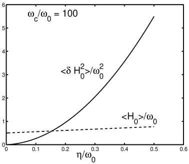
Figure 3.  : The mean energy $<H_{0}>$ (broken line) of the oscillator and the instantaneous mean-squared energy fluctuations $<\delta H^{2}_{0}>=<(H_{0}(t)-<H_{0}>)^{2}>$ in the ground state of the Lamb model as a function of the coupling constant $\eta$ in units with $\hbar=1$. After K. Nagaev and M. Büttiker [20].

The mean-squared fluctuations of the energy of the oscillator are shown in Fig. 3 as a function of $\eta$ (over a range exceeding the limit of validity of Eq. (11)). We have emphasized the possibility of energy fluctuations in the ground state, since following Ref. [12], the possibility of such fluctuations was questioned in Ref. [21].

It is perhaps necessary to point out the following: In standard statistical mechanics it is assumed that the coupling energy is always smaller than any relevant energy scale of the system under consideration [22]. Thus in standard statistical mechanics the only properties of the bath which enter are the temperature and the chemical potential of the bath. Here in contrast, the friction constant $\eta$ enters in a non-trivial way. We next aim at characterizing the vacuum state of the bath.

4 Traces in the bath

In theories of decoherence [23, 24] the trace which a system leaves in the environment plays an important role. Zurek compares this to the waves a ship leaves in its wake while crossing a sea [23]. Since the vacuum is not a quiet state, we can ask: Does the oscillator leave a trace in the bath even in the ground state of the system? And if the answer is yes, what are the properties of this trace?

First, let us characterize the incoming field. The noise force $2V_{L}(t)=-2RdQ_{L}(t)/dt$ (see Eq. (2)) which acts on the harmonic oscillator is determined by the voltage drop across the oscillator generated by the incident (left moving) field. Thus we will discuss the state of the bath by investigating the voltages generated by the left and right moving traveling fields.

A simple calculation gives for the correlation $S_{V_{L}V_{L}}(t)\equiv\langle 0|V_{L}(t)V_{L}(0)+V_{L}(0)V_{L}(t)|0\rangle$

$$S_{V_{L}V_{L}}(t)=\frac{\hbar R}{4\pi}\,\int_{-\infty}^{\infty}d\omega|\omega|\,\exp(-i\omega t)\exp(-\omega/\omega_{c})=$$

$$\frac{1}{e^{2}}\,\frac{R}{R_{K}}\,\frac{(\hbar\omega_{c})^{2}}{2\pi}\frac{1-\omega_{c}^{2}t^{2}}{(1+\omega_{c}^{2}t^{2})^{2}}.$$ (12)

Here we have introduced the resistance quantum $R_{K}=h/e^{2}$. The correlation is positive at very short times $t<1/\omega_{c}$ but negative at long times with a decay proportional to $t^{-2}$. This property is a consequence of the particular frequency dependence of the noise power spectral density of the vacuum fluctuations. The spectral density is

$$<0|V_{L}(\omega)V_{L}(\omega^{\prime})+V_{L}(\omega^{\prime})V_{L}(\omega)|0>=2\pi S_{V_{L}V_{L}}(\omega)\,\delta(\omega+\omega^{\prime})$$ (13)

where $V(\omega)$ is the Fourier transform of $V(t)$. The vacuum fluctuations of the force are characterized by a spectral density

$$S_{V_{L}V_{L}}(\omega)=\hbar|\omega|\,R/4$$ (14)

Now since the incoming field $V_{L}(x/v+t)$ differs from the field at $x=0$ only by a phase factor multiplying each operator, Eq. (14) gives also the spectral density of the voltage correlation $<0|V_{L}(x,t)V_{L}(x,0)+V_{L}(x,0)V_{L}(x,t)|0>$. at any other point $x$ along the chain. Next consider the voltage $V_{R}(x/v-t)$ generated by the right movers. Its spectral density is also given by Eq. (14). Both the left and right goers are characterized by the same spectral density.

To find the trace which the system leaves in the environment we have to consider the correlations between the voltage fluctuations generated by the incident field and the voltage fluctuations of the out-going field. We find that these correlations have a spectral density

$$S_{V_{L}V_{R}}(\omega)=S_{V_{R}V_{L}}(-\omega)=(\hbar Z/4)\,|\omega|\,s(\omega)$$ (15)

where $s$ is the scattering matrix given by Eq. (7).

The spectrum of the total voltage fluctuations (which contains the correlations between left and right movers) exhibits a dramatic effect. From the spectral densities of the incoming voltage fluctuations and the outgoing voltage fluctuations we can calculate the spectrum of the total voltage fluctuations, $V=V_{L}+V_{R}$ for which we find,

$$S_{VV}(\omega)=(\hbar|\omega|R/2)\,(2+s(\omega)+s(-\omega))$$ (16)

which with the $s$-matrix, Eq. (7) gives

$$S_{VV}(\omega)=R\,\hbar|\omega|\,\frac{(\omega^{2}-\omega^{2}_{0})^{2}}{(\omega^{2}-\omega^{2}_{0})^{2}+\eta^{2}\omega^{2}}.$$ (17)

At resonance, for $\omega=\pm\omega_{0}$, the spectral density of the total voltage fluctuations vanishes. This reflects the fact that at resonance our system can not maintain a voltage drop.

Eq. (17) can be simply derived from an equivalent electrical circuit. We replace the transmission line by a resistor with resistance $R$ in parallel with a current noise source with current $I_{N}$. The current noise source has a spectral density

$$S_{I_{N}I_{N}}(\omega)=(1/R)\,\hbar|\omega|\,coth(\hbar\omega/2kT).$$ (18)

Here we have for later reference given the finite temperature result. Unless stated otherwise we continue to discuss the zero-temperature limit only. The current through the ”system” (the LC-oscillator) is $I_{s}=V/Z_{s}$. Here $Z_{s}=(-i\omega C)^{-1}-i\omega L$ is the impedance of the system as seen from the noise source. The current through the resistance is $I=V/R$. Current conservation demands $I_{s}+I+I_{N}=0$ and together with Eq. (18) leads immediately to the spectral density Eq. (17) for the voltage $V$.

Thus far we have considered a harmonic oscillator at zero-temperature coupled to a bath. We have shown that its energy fluctuates and have examined the trace it leaves in the bath. This trace has its source in the time-delay suffered by vacuum fluctuations due to their interaction with system. Next we now consider two level systems coupled to a bath and consider dephasing and and decoherence in these systems.

5 Two-Level Systems

A large class of physically interesting systems can be reduced to an effective two-level problem. We consider systems which in the absence of a bath are described by the Hamiltonian

$$H_{0}=\frac{\hbar\epsilon_{0}}{2}\,\sigma_{z}-\frac{\hbar\Delta_{0}}{2}\,\sigma_{x}$$ (19)

where $\hbar\epsilon_{0}$ is the energy difference between two levels (in the absence of tunneling), and $\Delta_{0}$ is a tunneling frequency which hybridizes the two levels. The energy of the ground state and the excited state of this system are

$$E_{\mp}=\mp\frac{\hbar\Omega_{0}}{2}=\mp\frac{\hbar}{2}\sqrt{\epsilon_{0}^{2}+\Delta_{0}^{2}}$$ (20)

where we have introduced the frequency $\Omega_{0}$. The two energy levels are shown in Fig. 4 as a function of $\epsilon_{0}$. The coupling energy is

$$H_{c}=g\frac{eV}{2}\,\sigma_{z}$$ (21)

where $g$ is a dimension less coupling constant and $V$ is the voltage which drops across the system. The total Hamiltonian contains in addition the contribution from all the energies of the bath oscillators.

Figure 4.  : Energy levels of the two state system in the presence of tunneling ($\Delta_{0}\neq 0$) and in the absence of tunneling ($\Delta_{0}=0$).

To be specific we consider the electrical system shown in Fig. 5. A small mesoscopic ring is formed by a quantum dot which is coupled via tunnel barriers with transmission amplitudes $t_{L}$ and $t_{R}$ to leads. The leads are connected back onto themselves such that they form together with the dot a ring structure. An Aharonov-Bohm flux $\Phi$ penetrates the hole of the ring. The model without the external circuit is discussed in Ref. [11]. The role of the external circuit (the bath) is the subject of Refs. [12, 25, 26]. A ballistic ring coupled to the electromagentic vacuum fields is investigated in Ref. [27]. In our geometry, the quantum dot generates a system that is highly sensitive to fluctuations of the environment. A completely equivalent model consists of a superconducting electron box [28] which can be opened to admit an Aharonov-Bohm flux [29, 30].

Figure 5.  : Ring with an in-line dot subject to a flux $\Phi$ and capacitively coupled to an external impedance $Z$. After [12, 26].

The arm of the ring contains electrons in levels with energy $E_{am}$ and the dot contains electrons in levels with energy $E_{dn}$. First let us for a moment neglect tunneling. Let $F_{N}$ be the free energy for the case that there are $N$ electrons in the dot and $M$ electrons in the arm. The transfer of an electron from the arm to the dot gives a free energy $F_{N+1}$. The difference of these two free energies is

$$\hbar\epsilon_{0}=F_{N+1}-F_{N}=E_{d(N+1)}-E_{aM}+\frac{e^{2}(N+1/2-C_{0}V_{e})}{C}.$$ (22)

Here the first two terms arise from the difference in kinetic energies. The third term results from the charging energy of the dot. $C^{-1}_{0}=C^{-1}_{i}+C^{-1}_{e}$ is the series capacitance of the internal capacitance $C_{i}=C_{L}+C_{R}$ and the external capacitance $C^{-1}_{e}=C^{-1}_{1}+C^{-1}_{2}$. The total capacitance is $C=C_{i}+C_{e}$. Eq. (22) measures the distance to resonance, $\epsilon_{0}=0$ is the condition that the Coulomb blockade is lifted [31].

Tunneling through the barriers connecting the dot and the arm is described by amplitudes $t_{L}$ and $t_{R}$. The total tunneling energy through the dot depends on these amplitudes and the Aharonov-Bohm flux $\Phi$ in the following way,

$${\hbar\Delta_{0}\over 2}=\sqrt{t_{L}^{2}+t_{R}^{2}\pm 2t_{L}t_{R}\cos{2\pi\Phi\over\Phi_{0}}},$$ (23)

where $\Phi_{0}=hc/e$ is the single electron flux quantum. The sign depends on the number of electrons in the dot and arm: it is positive, the total number is odd, and it is negative if the total number is even [11]. The voltage across the system is $V=V_{0}-V_{\infty}$. The coupling constant in $H_{c}$ is $g=C_{0}/C_{i}$.

In the two-level limit of interest here the transmission amplitudes $t_{L}$ and $t_{R}$ are taken to be very small compared to the level spacing in the dot and in the arm. For larger transmission amplitudes the system without a bath will already exhibit a Kondo effect [32, 33, 34, 35].

There are two important classes of two-level systems, depending on whether $\sigma_{z}$ commutes with the total Hamiltonian or not.

6 Two-level systems with a coherent ground state

Consider the case of vanishing tunneling frequency $\Delta_{0}=0$. In this case $[H,\sigma_{z}]=0$. As a consequence a pure state state of $H_{0}$ remains a pure state also in the presence of the coupling to the bath.

This model is most often used to investigate the decoherence of superpositions of two states. We discuss this briefly even though our main interest is in the coherence properties of the ground state and not of the excited states of the system. The state of the system can be written as a spinor with angles $\theta$ and $\phi$ on the Bloch sphere,

$$|\Psi>=\left(\begin{array}[]{ll}\cos(\theta/2)\,\exp(i\phi/2)\\ \sin(\theta/2)\,\exp(-i\phi/2)\end{array}\right).$$ (24)

This state represents a superposition of a spin up state $|\uparrow>={0\hfill\choose 1},$ and a spin down state $|\downarrow>={1\hfill\choose 0},$ with

$$|\psi>=\cos(\theta/2)\,\exp(i\phi/2)|\uparrow>+\sin(\theta/2)\,\exp(-i\phi/2)|\downarrow>.$$ (25)

In the absence of a bath the spin precesses with a Larmor frequency $\omega_{L}=\epsilon_{0}$ around the $z$-axis, such that $\theta=const$ and $\phi=-\omega_{L}t$. If the system is coupled to the bath it is still possible to find an exact solution of the full problem for arbitrary coupling strength. Palma, Souminen and Ekert [5] discuss this in terms of displaced bath oscillators. Here, to find this solution we proceed by looking at the problem from an electrical circuit point of view and derive a simple Langevin equation. As briefly discussed in Section 4, we can represent the bath by a resistor $R$ in parallel with a noise source with current $I_{N}(t)$ with a spectral density given by Eq. (18).

Using the spinor Eq. (24) with $\phi(t)=-\omega_{L}t+\delta\phi(t)$, where $\delta\phi(t)$ accounts for the fluctuations in the phase, we find from the Hamiltonian the equation

$$\frac{d\delta\phi(t)}{dt}=\frac{e}{\hbar}\,\frac{C_{0}}{C_{i}}\,V(t)$$ (26)

Next we need to find the voltage which drops across this two-level system. The current through the resistor is $V/R$, the current through the system is $C_{0}dV(t)/dt$ and the current of the noise source in parallel to the resistor is $I_{N}(t)$ and therefore,

$$V=-RC_{0}\,dV(t)/dt+R\,I_{N}(t).$$ (27)

Scattering of the incident vacuum states at this system is described by an s-matrix $s=-(1+i\omega\tau)/(1-i\omega\tau)$ which is the overdamped limit $\omega^{2}\ll\omega_{0}^{2}$ of Eq. (7). Here $\tau=\eta/\omega_{0}^{2}=RC_{0}$ is the $RC$-time of the electrical circuit. Taking the Fourier transform of Eqs. (26) and (27) gives for the spectral density of the voltage fluctuations

$$S_{VV}(\omega)=\frac{R\hbar|\omega|}{1+\omega^{2}\tau^{2}}$$ (28)

and for the phase fluctuations

$$S_{\phi\phi}(\omega)=\frac{e^{2}}{\hbar^{2}}\,\frac{C_{0}^{2}}{C_{i}^{2}}\,\frac{1}{\omega^{2}}\,\frac{R\hbar|\omega|}{1+\omega^{2}\tau^{2}}.$$ (29)

The spectrum is proportional to $1/|\omega|$ at low frequencies. Consider next the density matrix. We have

$${\bf\rho}=\left(\matrix{\cos^{2}(\theta/2)&(1/2)\sin(\theta)\,\exp(i\phi)\cr(1/2)\sin(\theta)\,\exp(-i\phi)&\sin^{2}(\theta/2)}\right).$$ (30)

Since the fluctuations $\delta\phi(t)$ are Gaussian (as is known for a harmonic oscillator coupled to a bath) we find that the averaged density matrix evolves away from its initial value at $t=0$ according to $<\exp(i\phi)>=$ $\exp(-i\omega_{L}t)$ $\exp(-\Gamma(t))$ where

$$\Gamma(t)=(1/2)<(\phi(t)-\phi(0))^{2}>.$$ (31)

With the help of the spectral density Eq. (29) we find the mean-square deviation of the phase away from its initial value,

$$\Gamma(t)=(1/\pi)\int d\omega\,S_{\phi\phi}(\omega)\,\sin^{2}(\omega t/2).$$ (32)

Thus $\Gamma(t)$ determines the decoherence of a superposition of the two states of the two-level system. Our spectrum Eq. (28) has a natural cut-off due to lorentzian role-off of the spectrum with the $RC_{0}$-time. This gives $\Gamma(t)\propto(t/\tau)^{2}$ for $t\ll\tau$ and gives $\Gamma(t)\propto\ln(t/\tau)^{2}$ at long times, and thus an approximate expression covering both the short and long time behavior is

$$\Gamma(t)\approx 2\alpha\,\ln\left(1+(t/4\tau)^{2}\right).$$ (33)

where we have introduced the coupling parameter

$$\alpha\equiv{R\over R_{K}}\,\left({C_{0}\over C_{i}}\right)^{2}.$$ (34)

Here $R_{K}=h/e^{2}$ is the von Klitzing resistance quantum. For $t>\tau$ the decay of the two state superposition is $\exp(-\Gamma(t))\propto t^{-2\alpha}$.

To summarize: the two-level system with $\Delta_{0}=0$ is a simple example with a coherent ground state. Superpositions of the ground state and the excited state decay due to the vacuum fluctuations of the bath. This model exhibits no population decay (the diagonal elements of the density matrix are constants of motion). Initial off-diagonal elements of the density matrix vanish over time due vacuum fluctuations. Next we consider the case of a two-level system with a tunneling frequency given by $\Delta_{0}$.

7 Two-level systems with a partially coherent ground state

In the presence of an Aharonov-Bohm flux the ground state of the ring-dot system shown in Fig. 5 permits a persistent current if the two tunneling amplitudes $t_{L}$ and $t_{R}$ are non-vanishing. If we consider for a moment the system decoupled from the bath, the free energy ( apart from an unimportant constant) is

$$\Delta F=-\frac{\hbar}{2}\sqrt{\epsilon_{0}^{2}+\Delta_{0}^{2}}\equiv-\frac{\hbar\Omega_{0}}{2}.$$ (35)

The second equality defines the frequency $\Omega_{0}$. Its derivative with respect to an Aharonov-Bohm flux $\Phi$ gives an equilibrium, ground state current, given by [11]

$$<I>=-c\frac{d\Delta F}{d\Phi}=\mp\,{e}\frac{4\pi t_{L}t_{R}}{\Omega_{0}}\,\sin(2\pi\Phi/\Phi_{0}).$$ (36)

The equilibrium current is a pure quantum effect: only electrons whose wave functions are sufficiently coherent to reach around the loop contribute to the persistent current. Thus the persistent current is a measure of the coherence of the ground state. At resonance $\epsilon=0$ the current is of the order of $et$ with $t$ a transmission amplitude and it decreases and becomes of the order of $et^{2}/\epsilon$ as we move away from resonance.

Figure 6.  : The persistent current $<I>$ at resonance $\epsilon=0$ for a symmetric ring (solid line) and the fluctuations of the circulating current $(<(I(t)-<I(t)>)^{2}>)^{1/2}/<I>$ (dashed line) as a function of the coupling parameter $\alpha$. The average persistent current is in units of the persistent current at $\alpha=0$. The fluctuations are normalized by the average current. The parameters are $\omega_{c}=25\Delta_{0}$. After [12].

Therefore, it is interesting to ask how this current is affected if the system is coupled to a bath. In contrast to the two-level problem in the absence of tunneling, the two-level problem of interest here, is not exactly solvable. Cedraschi, Ponomarenko and the author [12, 25] used known solutions from a Bethe ansatz and perturbation theory to provide an answer. In addition these authors also investigated the (instantaneous) fluctuations of the equilibrium current away from its average, $<(I(t)-<I(t)>)^{2}>$. For the symmetric case $t_{L}=t_{R}$, $C_{L}=C_{R}$, the average current together with the mean-squared current fluctuations is shown in Fig. 6 as a function of the coupling parameter $\alpha$ (see Eq. (34)). The persistent current is in units of the current for $\alpha=0$. A similar, but very weak, reduction of the persistent current has also been found for a purely ballistic ring coupled to the electromagnetic vacuum fields [27]. In Fig. 6 the mean squared current fluctuations $(<(I(t)-<I(t)>)^{2}>)^{1/2}$ are in units of the average current $<I(t,\alpha)>$. With increasing resistance we have thus a cross over from a state with a well defined persistent current (small mean-squared fluctuations) to a fluctuation dominated state in which the mean-squared fluctuations of the persistent current are much larger than the average persistent current. For the derivation of these results we refer the reader to Refs. [12] and [25].

Here we pursue a discussion based on Langevin equations [26] similar to the approach described above. This approach is valid only for weak coupling constants $\alpha\ll 1$ but has the benefit of being simple.

We want to find the time evolution of a state $\psi(t)$ of the two-level system in the presence of the bath. We write the state of the two-level system

$$\psi=e^{i\chi/2}{\cos{\theta\over 2}\,e^{i\varphi/2}\hfill\choose\sin{\theta\over 2}\,e^{-i\varphi/2}},$$ (37)

with $\theta$, $\varphi$ and $\chi$ real. This is the most general form of a normalized complex vector in two dimensions. In terms of $\theta$, $\varphi$ and the global phase $\chi$, the time dependent Schrödinger equation reads [26]

$$\dot{\varphi} = -\varepsilon_{0}-\delta\varepsilon(t)-\Delta_{0}\cot\theta\cos\varphi,$$ (38)

$$\dot{\theta} = -\Delta_{0}\sin\varphi,$$ (39)

$$\dot{\chi} = \Delta_{0}{\cos\varphi\over\sin\theta}.$$ (40)

As shown by Eq. (40) the phase $\chi$ is completely determined by the dynamics of the phases $\theta$ and $\varphi$ and has no back-effect on the evolution of $\theta$ and $\varphi$. While $\chi$ is irrelevant for expectation values, like the persistent current or the charge on the dot, it plays an important role, in the discussion of phase diffusion times.

To close the system of equations we have now to find the voltage which drops across the system. In contrast to the two-level system discussed above in which the charge of the system is fixed, in the two-level system considered here the charge is permitted to tunnel between the dot and the arm of the ring. This charge transfer permits an additional displacement current through the system which we have to include to find the voltage fluctuations.

The charge operator on the dot for our effective two-level problem is

$$\hat{Q}_{d}=e\left(\matrix{1&0\cr 0&0}\right).$$ (41)

Its quantum mechanical expectation value is

$${Q}_{d}=\langle\psi(t)|\hat{Q}_{d}|\psi(t)\rangle=e\,\cos^{2}{\theta\over 2}.$$ (42)

The displacement current is proportional to the time-derivative of this charge, $\dot{Q}_{d}=-{e\over 2}\sin\theta\,\dot{\theta}$ multiplied by a ratio of capacitances which has to be found from circuit analysis. For this analysis we refer the reader to Ref. [26]. We find that the total current through the system is now given by $C_{0}\dot{V}-({C_{0}/C_{i}})({e/2})\sin\theta\,\dot{\theta}$. Using this result we find from the conservation of all currents (current through the system, the resistor and current of the noise source) that the fluctuating voltage across the system is determined by [26]

$$V=-C_{0}R\,\dot{V}-R\,{C_{0}\over C_{i}}\,{e\over 2}\,\sin\theta\,\dot{\theta}+RI_{N}(t).$$ (43)

Eqs. (38, 39) and (43) form a closed system of equations in which the external circuit is incorporated in terms of a fluctuating current $I_{N}(t)$ and of an ohmic resistor $R$. In the next section, we investigate Eqs. (38, 39) and (43) to find the effect of zero-point fluctuations on the persistent current of the ring.

8 Fluctuations of the ground state

First, let us discuss the stationary states of the system of differential equations, Eqs. (38, 39) and (43) in the absence of the noise term $I_{N}(t)$. We have $\sin\varphi=0$ and consequently a stationary state has $\varphi\equiv\varphi_{0}$, with $\varphi_{0}=0$ or $\varphi_{0}=\pi$. With this it is easy to show that in the stationary state we must have $\theta\equiv\theta_{0}$, with

$$\cot\theta_{0}=\pm{\varepsilon_{0}\over\Delta_{0}}.$$ (44)

The lower sign applies for $\varphi_{0}=0$. This is the ground state for the ring-dot system at fixed $\varepsilon(t)\equiv\varepsilon_{0}$, and the upper sign holds for $\varphi_{0}=\pi$. The energy of the ground state is $-\hbar\Omega_{0}/2$, thus the global phase is $\chi_{0}(t)=\Omega_{0}t$ where $\Omega_{0}$ is the resonance frequency of the (decoupled) two-level system (see Eq. (35)). We also introduce the “classical” relaxation time $\tau_{RC}\equiv RC_{0}$, and a rate

$$\Gamma\equiv\pi\alpha{\Delta_{0}^{2}\over\Omega_{0}}$$ (45)

which as we shall see is a relaxation rate due to the coupling of the ring-dot system to the external circuit. $\alpha$ is the dimensionless coupling constant introduced above (see Eq. (34)).

Now, we switch on the noise $I_{N}(t)$. We seek $\varphi(t),\theta(t)$, $\chi(t)$ and $V(t)$ to linear order in the noise current $I_{N}(t)$. We expand $\varphi(t)$ and $\theta(t)$ to first order around the ground state, $\varphi=0$ and $\theta=\theta_{0}$. For $\delta\varphi(t)=\varphi(t)-\varphi_{0}$, $\delta\theta(t)=\theta(t)-\theta_{0}$, we find in Fourier space,

$$-i\omega\delta\varphi = -\delta\varepsilon+{\Omega_{0}^{2}\over\Delta_{0}}\,\delta\theta,$$ (46)

$$-i\omega\delta\theta = -\Delta_{0}\,\delta\varphi,$$ (47)

$$-i\omega\,\delta\varepsilon = {1\over\tau_{RC}}\left[-\delta\varepsilon-\Gamma\,\delta\varphi+{e\over\hbar}\,R\,{C_{0}\over C_{i}}\,I_{N}\right].$$ (48)

We also expand the global phase $\chi(t)$ around its evolution in the ground state $\chi_{0}(t)=\Omega_{0}t$, and define $\delta\chi(t)=\chi(t)-\chi_{0}(t)$. In Fourier space, Eq. (40) becomes

$$-i\omega\delta\chi=\Omega_{0}\,{\varepsilon_{0}\over\Delta_{0}}\delta\theta.$$ (49)

We note that there is no effect of the global shift in energy, $\hbar\nu(t)$, as it is quadratic in the voltage $\delta V$, and we are only interested in effects up to linear order in $\delta V$.

9 Mapping onto a harmonic oscillator

Let us assume that the charge relaxation time of the external circuit $\tau_{RC}$ is very short compared to the dynamics of the two-level system $\tau_{RC}\ll\Omega_{0}$. Eliminating $\delta\theta$ with the help of Eq. (47) and $\delta\varepsilon$ with the help of Eq. (48) we find

$$(\omega^{2}-i\omega\Gamma-\Omega_{0}^{2})\,\delta\theta=\Delta_{0}\,{e\over\hbar}\,{C_{0}\over C_{i}}\,R\,I_{N}.$$ (50)

Thus we have mapped the dynamics of the fluctuations away from the ground state of this two-level system on the Langevin equation of a damped harmonic oscillator subject to quantum fluctuations. $\delta\theta$ plays the role of the charge, $\delta\varphi$ the role of the current and $\Gamma$ takes the role of the friction constant in the $LC$-oscillator discussed in Section 2. We can now immediately use the results of the first few sections of this work to describe the fluctuations in the ground state of this two-level problem. The spectral density $S_{\theta\theta}(\omega)$ is just that of the coordinate of the harmonic oscillator or that of the charge of the $LC$-oscillator,

$$S_{\theta\theta}(\omega)={2\pi\,\alpha\,\Delta_{0}^{2}\,|\omega|\over\left[\left(\omega^{2}-\Omega_{0}^{2}\right)^{2}+\Gamma^{2}\omega^{2}\right]}.$$ (51)

Note that the intensity of the noise power is proportional to $\Delta_{0}^{2}$. Alternatively we could write the intensity as $\pi\alpha\Delta_{0}^{2}=\Omega_{0}\Gamma$.

The approach presented here is valid only in the weak coupling limit. The poles of the weakly damped oscillator are

$$\omega_{\pm}=\pm\Omega_{0}-i{\Gamma\over 2},$$ (52)

and we can write

$$S_{\theta\theta}(\omega)={2\pi\,\alpha\,\Delta_{0}^{2}|\,\omega|\over\left[\left(\omega-\Omega_{0}\right)^{2}+\left(\Gamma/2\right)^{2}\right]\left[\left(\omega+\Omega_{0}\right)^{2}+\left(\Gamma/2\right)^{2}\right]}.$$ (53)

Expressing the spectrum as a sum of separate pole contributions we find

$$S_{\theta\theta}(\omega)=\frac{2\pi\,\alpha\,\Delta_{0}^{2}}{\Omega_{0}}\left(\frac{1-((\omega-\Omega_{0})/4\Omega_{0})}{\left[\left(\omega-\Omega_{0}\right)^{2}+\left(\Gamma/2\right)^{2}\right]}+\frac{1+((\omega+\Omega_{0})/4\Omega_{0})}{\left[\left(\omega+\Omega_{0}\right)^{2}+\left(\Gamma/2\right)^{2}\right]}\right).$$ (54)

The factors ${1\mp(\omega\mp\Omega_{0})/4\Omega_{0}}$ account for the effect of the Lorentzian tails of the far away pole.

In the literature [36, 37, 38] it is often the correlation function of $\sigma_{z}$ which is of interest. We have $<\psi|\sigma_{z}|\psi>=\cos(\theta)$ and thus for the fluctuations away from the average $\Delta<\psi|\sigma_{z}|\psi>=-\sin(\theta_{0})\delta\theta$. Since $\sin(\theta_{0})=\Delta_{0}/\Omega_{0}$, we find in the zero-temperature limit $S_{\sigma_{z}\sigma_{z}}(\omega)=(\Delta^{2}_{0}/\Omega^{2}_{0})S_{\theta\theta}(\omega)$. This result agrees with an expression given by Weiss and Wollensak [36] and Görlich et al. [37] who have used an entirely different approach. For non-zero temperatures Weiss and Wollensak find in addition a peak around zero-frequency: This is a Debye relaxation peak and in the discussion given here it is not included. We have expanded around the (time-independent) ground state of the decoupled system. To find the Debye relaxation peak from a weak coupling treatment it is necessary to consider the relaxation towards the instantaneous (time-dependent) state of the system. At temperatures $kT\ll\hbar\Omega_{0}$ the weight of the Drude peak is exponentially small. The result of Weiss and Wollensak also includes a temperature dependent renormalization of the bare pole frequencies $\Omega_{0}$. The most essential point for the discussion here, is however, the fact that the peaks are broadened with a relaxation rate $\Gamma$. The spectrum Eq. (54) is that of the coordinate (or charge) of a weakly damped harmonic oscillator subject to quantum fluctuations.

Using Eqs. (47) and (48) we obtain similarly the spectral densities $S_{\varphi\varphi}(\omega)$, $S_{\chi\chi}(\omega)$ and cross-correlations like $S_{\theta\varphi}(\omega)$.

10 Suppression of the Persistent current

Let us next examine the reduction of the persistent current using the approach outlined above. To be brief we consider only the case of a symmetric ring $t_{R}=t_{L}\equiv t$ and $C_{R}=C_{L}$ (see Fig. 5). The persistent current is the quantum and statistical average of the operator

$$\hat{I}_{c}={\cal J}\sigma_{z}$$ (55)

where $\cal J$ is given by

$${\cal J}={\hbar c}{\partial\Delta_{0}\over\partial\Phi}.$$ (56)

In general, in the non-symmetric case, the operator for the persistent current depends also on the capacitances (see Appendix B of Ref. [26]).

The quantum mechanical expectation value of the persistent current for the state given in Eq. (37) reads

$$I(t)\equiv\langle\psi(t)|\hat{I}_{c}|\psi(t)\rangle={1\over 2}{\rm Re}\,({\cal J}\sin\theta\,e^{-i\varphi}).$$ (57)

We are interested in the statistically averaged persistent current $\langle I(t)\rangle$. Therefore, we have to calculate the correlator $\langle\sin\theta\,e^{-i\varphi}\rangle$. First, we observe that there are no correlations between $\delta\varphi$ and $\delta\theta$. The symmetrized correlation function $\langle\delta\varphi(t)\delta\theta(t)\rangle=0$, since the spectral density $S_{\varphi\theta}(\omega)$ is an odd function of $\omega$. (This statement is equivalent to the vanishing of the correlations between $p$ and $q$ for a harmonic oscillator). For a harmonic oscillator the fluctuations are Gausssian and thus within the range of validity of our discussion there are no correlations to all orders in $\theta(t)$ and and $\varphi(t)$. Thus we have $\langle\sin\theta e^{-i\varphi}\rangle=\langle\sin\theta\rangle\langle e^{-i\varphi}\rangle$. and

$$\langle e^{-i\varphi(t)}\rangle=e^{-i\varphi_{0}}\langle e^{-i\delta\varphi(t)}\rangle=\exp\left(-{\left\langle\delta\varphi^{2}(t)\right\rangle\over 2}\right),$$ (58)

where we have used that $\varphi_{0}=0$. In the weak coupling limit, and in the extreme quantum limit, $T=0$, we find for the time averaged mean-squared fluctuations to leading order in $\Gamma$,

$$\langle\delta\varphi^{2}(t)\rangle=\int_{0}^{\omega_{c}}\frac{d\omega}{\pi}S_{\varphi\varphi}(\omega)=\frac{\Omega_{0}}{\Delta_{0}^{2}}[2\Gamma\ln{\omega_{c}\over\Omega_{0}}-\Gamma+\pi\Omega_{0}]\approx 2\alpha\ln{\omega_{c}\over\Omega_{0}}.$$ (59)

Here we have assumed that the cut-off frequency is so large that the logarithmic term dominates. In the limit $\omega_{c}\gg\Omega_{0}$, we can neglect $\langle\delta\theta^{2}(t)\rangle=\int_{0}^{\omega_{c}}(d\omega/\pi)S_{\theta\theta}(\omega)$ against $\langle\delta\varphi^{2}(t)\rangle$. We insert $\langle\delta\varphi^{2}(t)\rangle$ and $\sin\theta_{0}=\Delta_{0}/\Omega_{0}$ into $\langle\sin\theta\,e^{-i\varphi}\rangle$, and find a noise averaged persistent current in the ring given by

$$\langle I(t)\rangle=-{\hbar c\over 2}{\partial\Delta_{0}\over\partial\Phi}{\Delta_{0}\over\Omega_{0}}\left({\Omega_{0}\over\omega_{c}}\right)^{\alpha}.$$ (60)

The weak coupling limit corresponds to $\alpha\ll 1$. The power law for the persistent current obtained in Eq. (60), as well as the exponent $\alpha$, Eq. (34) coincide in this limit with the result obtained by using a Bethe ansatz solution. Cedraschi et al. [12] found for $\alpha<1$ that at resonance ($\epsilon=0$) the persistent current is given by $I(\varepsilon=0)\propto\left({\Delta_{0}/\omega_{c}}\right)^{\alpha/(1-\alpha)}.$ For a small coupling parameter, $\alpha\ll 1$, the Bethe ansatz result goes over to the power law of Eq. (60). Thus, if it can be assumed that the logarithmic term dominates in Eq. (59), the simplified discussion presented here leads, at least in the weak coupling limit, to the same result as the one obtained in Ref. [12].

We emphasize that the persistent current is a property of the ground state of a system. In our case, the persistent current is, however, carried by only a part of the system. Due to the coupling to the external circuit this subsystem is subject to fluctuations which even at zero temperature suppress the persistent current. If we keep the capacitances fixed, Eq. (60) gives a persistent current which decreases with increasing external resistance $R$.

For the case considered here it is simple to also discuss the instantaneous fluctuations of the persistent current. From Eq. (55) we find $\hat{I}_{c}^{2}={\cal J}^{2}{\bf 1}$ where ${\bf 1}$ is the unit matrix. Thus the mean squred fluctuations $(\Delta I)^{2}=(\hat{I}_{c}-\langle I(t)\rangle)^{2}$ of the persistent current are

$$\langle(\Delta I)^{2}\rangle={\cal J}^{2}-(\langle I(t)\rangle)^{2}$$ (61)

Thus with increasing coupling constant $\alpha$ the average persistent current decreases and the mean squared fluctuations of the persistent current increase (see also Fig. 6).

We next characterize the fluctuations of the angle variables of the ground state in more detail.

11 Phase Diffusion Times

Due to the vacuum fluctuations the ground state of the two-level system with tunneling is a dynamic state. To see this we project the actual state of the system on the ground state $\psi_{-}=(\cos\theta_{0}/2,\sin\theta_{0}/2)$, with energy eigenvalue $-\hbar\Omega_{0}/2$, and the excited state $\psi_{+}=(-\sin\theta_{0}/2,\cos\theta_{0}/2)$ with eigenvalue $\hbar\Omega_{0}/2$. Instead of the wave function $\psi(t)$ it is more convenient to consider $\psi_{R}(t)\equiv\exp(i\hat{H}_{0}t/\hbar)\psi(t)$. To first order in $\delta\varepsilon$, we find for the wave function $\psi_{R}$,

$$\psi_{R}(t)=(1+i\alpha)\psi_{-}+\beta\psi_{+}e^{i\Omega_{0}t}.$$ (62)

with

$$\alpha={\delta\chi(t)\over 2}-{\varepsilon_{0}\over\Omega_{0}}{\delta\varphi(t)\over 2}\,$$ (63)

$$\beta=\left[{\delta\theta(t)\over 2}-i{\Delta_{0}\over\Omega_{0}}{\delta\varphi(t)\over 2}\right]e^{i\Omega_{0}t}.$$ (64)

It is useful to write $\alpha(t)$ and $\beta(t)$ in terms of the Fourier amplitudes of the fluctuating phase $\phi(t)$. We find

$$\alpha(t)={1\over 2}{\varepsilon_{0}\over\Omega_{0}}\int{d\omega\over\omega^{2}}(\Omega_{0}^{2}-\omega^{2})\phi_{\omega}\exp(-i\omega t),$$ (65)

$$\beta(t)={1\over 2}{\Delta_{0}\over\Omega_{0}}\int{d\omega\over i\omega}(\Omega_{0}+\omega)\phi_{\omega}\exp(-i(\omega-\Omega_{0})t).$$ (66)

The term $\exp(i\Omega_{0}t)$ arises due to the energy difference between the ground state and the excited state. Thus the projection amplitudes $<\psi(t)|\psi_{-}(t)>=1+i\alpha(t)$ and $<\psi(t)|\psi_{+}(t)>=\beta(t)$ exhibit in time a mean-squared deviation away from their initial value given by

$$\left\langle\left|\alpha(t)-\alpha(0)\right|^{2}\right\rangle={\varepsilon_{0}^{2}\over\Omega_{0}^{2}}\int{d\omega\over 2\pi\omega^{4}}\sin^{2}{\omega t\over 2}(\Omega_{0}^{2}-\omega^{2})^{2}S_{\varphi\varphi}(\omega),$$ (67)

$$\left\langle\left|\beta(t)-\beta(0)\right|^{2}\right\rangle\approx{\Delta_{0}^{2}\over\Omega_{0}^{2}}\int{d\omega\over 2\pi}\sin^{2}{\omega t\over 2}S_{\varphi\varphi}(\omega+\Omega_{0})$$ (68)

The long time behavior of Eq. (67) is dominated by the frequencies near $\omega=0$. The spectral density $S_{\varphi\varphi}(\omega)$ vanishes like $\omega^{2}$ for finite temperatures or even like $|\omega|^{3}$ in the zero-temperature limit. For finite temperatures this gives raise to a long time behavior of the type $\langle|\alpha(t)-\alpha(0)|^{2}\rangle\sim t/\tau_{-}$, with a characteristic phase diffusion time

$$\tau_{-}={\hbar\over 2\pi\alpha\,kT}{\Omega_{0}^{2}\over\varepsilon_{0}^{2}}.$$ (69)

Note that this behavior arises from the fluctuations in the global phase $\chi$. Note also that $\tau_{-}$ depends on the detuning $\varepsilon_{0}$. In particular, at resonance $\varepsilon_{0}=0$, the phase diffusion time $\tau_{-}$ diverges for any temperature.

The long time behavior of Eq. (68), on the other hand, is determined by the frequencies near $\Omega_{0}$. In the vicinity of this characteristic frequency, $S_{\varphi\varphi}(\Omega_{0}+\omega)$ shows a $\omega^{-2}$ behavior at finite as well as at zero temperature, which is cut off by the relaxation rate $\Gamma$, defined in Eq. (45) at very small frequencies $\omega\sim\Gamma\ll\Omega_{0}$. We have, for $|\omega|\ll\Omega_{0}$

$$S_{\varphi\varphi}(\Omega_{0}+\omega)\approx{2\pi\alpha\,\Omega_{0}\coth{\hbar\Omega_{0}\over 2kT}\over\omega^{2}+(\Gamma/2)^{2}}.$$ (70)

The time evolution of Eq. (68) for times much larger than the inverse of the characteristic frequency $\Omega_{0}$, yet smaller than the inverse of the relaxation rate $\Gamma$, is therefore linear in time with a characteristic time $\tau_{+}$, where

$$\tau_{+}={1\over\Gamma}\tanh{\hbar\Omega_{0}\over 2kT}.$$ (71)

Note that Eq. (71) holds for finite temperatures as well as in the quantum limit. The phase diffusion time $\tau_{+}$ is inversely proportional to $T$ at high temperatures,

$$\tau_{+}={1\over\Gamma}{\hbar\Omega_{0}\over 2kT},\quad(kT\gg\hbar\Omega_{0}),$$ (72)

just as the other characteristic time $\tau_{-}$. In the low-temperature or quantum limit, however, it saturates to a value

$$\tau_{+}={1\over\Gamma},\quad(kT\ll\hbar\Omega_{0}).$$ (73)

The crossover from high temperature behavior to the quantum limit behavior takes place at $kT\sim\hbar\Omega_{0}$.

We emphasize that Eq. (67) and Eq. (68) do not hold for arbitrarily long times. In reality the mean-square displacements $\langle|\alpha(t)-\alpha(0)|^{2}\rangle$ and $\langle|\beta(t)-\beta(0)|^{2}\rangle$ are bounded since the wave function $\psi_{R}(t)$ is normalized to 1. The fact that Eq. (67) grows without bounds is an artifact of the linearization of Eqs. (38)–(40) and Eq. (43). The phase-diffusion rates $\tau_{-}$ and $\tau_{+}$ can be related to the relaxation rate and the dephasing time given by Weiss and Wollensak [36] and Grifoni, Paladino and Weiss [39]. To find the dephasing rate we write the time evolution of the state $\Psi_{R}(t)$ (see Eq. (54)) with the help of an overall phase $\eta(t)$ in the form $\Psi_{R}(t)=\exp(-i\eta(t))\Psi_{R}(0)$. For times scales over which $\eta$ remains small we have $\Psi_{R}(t)=(1-i\eta(t))\Psi_{R}(0)$ or $\Psi_{R}(t)-\Psi_{R}(0)=-i\eta(t)\Psi_{R}(0)$. The scalar product of $\Psi_{R}(t)-\Psi_{R}(0)$ with itself is $|\Psi_{R}(t)-\Psi_{R}(0)|^{2}=|\eta(t)|^{2}$ and its expectation value is thus just $<|\eta(t)|^{2}>=<|c_{-}(t)-c_{-}(0)|^{2}>+<|c_{+}(t)-c_{+}(0)|^{2}>$. The dephasing rate is $\Gamma_{\phi}=<|\eta(t)|^{2}>/2t$ and is therefore given by

$$\Gamma_{\phi}=\frac{1}{2\tau_{+}}+\frac{1}{2\tau_{-}}={\Gamma\over 2}\coth{\hbar\Omega_{0}\over 2kT}+{\pi\alpha\,kT\over\hbar}{\varepsilon_{0}^{2}\over\Omega_{0}^{2}}.$$ (74)

This dephasing rate, valid on short and intermediate times, saturates in the zero-temperature limit. At $kT=0$ we have $\Gamma_{\phi}=\Gamma/2$.

To summarize, we find that in a two-level system with tunneling, for which the Hamiltonian does not commute with the total Hamiltonian, phase-diffusion times $\tau_{-}$ and $\tau_{+}$, which are related to the projection of the equilibrium state $\psi(t)$ onto the ground state and the excited state. These rates also determine the dephasing rate. If we represent the state of the system as a spin, these results show that even in the ground state, the spin undergoes diffusion around the point on the Bloch sphere which it would mark in the absence of the bath. We have thus a problem for which the ground state exhibits only partial coherence.

12 Energy Fluctuations

It is interesting to compare the energy fluctuations of the two-level system with those of the harmonic oscillator in the Lamb model. Using the Bloch state vector Eq. (37) and the operator Eq. (19) for the system we find for the average energy

$$\langle\Psi|H_{0}|\Psi\rangle=(\hbar\epsilon_{0}/2)cos(\theta)-(\hbar\Delta_{0}/2)sin(\theta)cos(\phi).$$ (75)

For the ground state in the absence of the bath we have $\theta=\theta_{0}$ determined by $sin(\theta_{0})=\Delta_{0}/\Omega_{0}$ and $\phi=\phi_{0}=0$ and we find immediately, $\langle\Psi|H_{0}|\Psi\rangle=-\hbar\Omega_{0}/2$. If we know couple the system to the bath the angle variables fluctuate away from these values. To find the effect of these fluctuations we replace $\theta$ and $\phi$ in Eq. (75) by $\theta=\theta_{0}+\theta-\theta_{0}$ and $\phi=\phi_{0}+\phi-\phi_{0}$. We proceed as in the discussion of the persistent current and consider the fluctuations in $\theta$ as small compared to the fluctuations in $\phi$. Using $\langle cos(\theta-\theta_{0})\rangle>\approx 1$ and taking into account that $\phi_{0}=0$, we obtain,

$$\langle\Psi|H_{0}|\Psi\rangle=(\hbar\epsilon_{0}/2)cos(\theta_{0})-(\hbar\Delta_{0}/2)sin(\theta_{0})\langle cos(\phi-\phi_{0})\rangle.$$ (76)

Using Eqs. (58) and (59), assuming that the logarithmic term is dominant, we obtain,

$$\langle\Psi|H_{0}|\Psi\rangle=-\hbar\Omega_{0}/2+(\hbar\Delta_{0}^{2}/2\Omega_{0})(1-(\Omega_{0}/\omega_{c})^{\alpha}).$$ (77)

It is now easy to find the fluctuations in the energy of the two-level system. Using the expression of the energy operator Eq. (75) we find,

$$H_{0}^{2}=\frac{\hbar^{2}\Omega_{0}^{2}}{4}{\bf 1}$$ (78)

where ${\bf 1}$ is the unit matrix. Therfore, to leading order in the coupling constant, we find

$$\langle(\Delta E)^{2}\rangle=\langle\Psi|H_{0}^{2}|\Psi\rangle-\langle\Psi|H_{0}|\Psi\rangle^{2}=\frac{\hbar^{2}\Delta_{0}^{2}}{4}\left(1-\left(\frac{\Omega_{0}}{\omega_{c}}\right)^{\alpha}\right)$$ (79)

Thus the energy of a two-level system coupled to a bath fluctuates. The fluctuations increase rapidly with increasing coupling constant.

Measurements of energy fluctuations are possible: for instance (as done in optics) by resonantly exciting the system from one of the two levels to a still higher third level [40]. Clearly it would be very intersting to see such an experiment performed for two level systems in a mesoscopic system.

13 Discussion

In this work we have investigated the fluctuations of the ground state of a system coupled to a bath. We have emphasized that due to coupling to vacuum fluctuations the energy of a system is not sharp but fluctuates in time [12]. We have demonstrated this with an explicite calculation for an $LC$-oscillator coupled to a transmission line. Such energy fluctuations are not a consequence of absorption or emission of photons (real transitions) but simply reflect the fact that a normal mode of the uncoupled system is not a normal mode of the system coupled to the bath. Any appeal to purely statistical mechanics arguments which treats the system and bath modes as if they were uncoupled (neglects the coupling energy) simply misses this phenomenon. We have examined the trace which the system leaves in the environment. We have found that this trace has its origin in the correlations between the incident and the out-going vacuum field fluctuations.

We emphasize that the system-bath interaction is treated here in a non-perturbative way: even in the weak coupling limit the spectral densities which characterize the fluctuations of the angle variables of the ground state depend to all orders on the coupling constant. This is obviously very different form a perturbative treatment. Perhaps equally important is the following: Our model as an electronic interpretation: yet we do not start by considering, say the interaction of a single electron with a two-level fluctuator. Instead, as the transmission line illustrates, what is considered is the interaction of plasmon waves (collective excitations) with the two-level system.

We have investigated the decoherence of a two-level system for which the Hamiltonian of the system commutes with the total Hamiltonian. This in an example of a system in which the ground state remains a pure state even in the presence of the bath. Superpositions of the ground state and the excited state decoher due to vacuum fluctuations without energy transfer [5] although only inversely proportional to a power law in time. The main focus in this work has been on a simple model system with tunneling for which the Hamiltonian of the system does not commute with the total Hamiltonian. The persistent current provides a measure of the coherence of the ground state and is suppressed with increasing coupling to the bath. In the weak coupling limit, in the ground state, the system exhibits a spectral density for the fluctuations of the angles of the spin on the Bloch sphere which is that of a damped harmonic oscillator subject to vacuum fluctuations. This enabled us to show that on short and intermediate times this system undergoes diffusion on the Bloch sphere even in the ground state. We have thus a system with a ground state that is only partially coherent.

What are the implications of these results for the discussion of the dephasing times in mesoscopic physics? The fact that the commutation of the systems Hamiltonian with the total Hamiltonian determines in the above mentioned examples whether or not we have a coherent ground state is possibly a general rule with which we can decide whether to expect a dephasing rate which tends to zero with temperature or a dephasing rate which saturates. In weak localization an electron and its time-reversed companion are the ”system” and all the other electrons, together with the electromagnetic interaction, provide the bath. Does the Hamiltonian of the quasi particles commute with the total Hamiltonian? Since weak localization also invokes an ensemble averaging procedure the answer to this question is not obvious.

Vacuum fluctuations have played a key role in the development of quantum mechanics. Our increasing ability to make small systems and measure them makes it likely that these fluctuations will continue to be of high interest.

References

- [1] P. W. Milloni, The Quantum Vacuum, (Academic Press, Boston, 1994).
- [2] A. J. Leggett, S. Chakravarty, A. T. Dorsey, M. P. A. Fisher and W. Zwerger, Rev. Mod. Phys. 59, 1 (1987).
- [3] U. Weiss, Quantum Dissipative Systems, (Word Scientific, 2000).
- [4] I. L. Aleiner, B. L. Altshuler, and M. E. Gershenson, Waves in Random Media 9, 201 (1999).
- [5] G. M. Palma, K.-A. Souminen, and A. Ekert, Proc. Royal Soc. London, A 452, 567 (1996).
- [6] P. Mohanty, E. M. Q. Jariwala, and R. A. Webb, Phys. Rev. Lett. 78, 3366 (1997).
- [7] P. Mohanty, Ann. Physik 8, 549 (1999).
- [8] D. S. Golubev and A. D. Zaikin, Phys. Rev. Lett. 82, 3191 (1999); A. D. Zaikin and D. S. Golubev, Physica B 280, 453 (2000).
- [9] I. L. Aleiner, B. L. Altshuler, and M. E. Gershenson, Phys. Rev. Lett. 82, 3190 (1999).
- [10] D. Natelson, R. L. Willett, K. W. West, and L. N. Pfeiffer, Phys. Rev. Lett. 78, 1821 (2001). A large set of closely related experiments is reported by J. J. Lin and L. Y. Kao, J. Phys. Condens. Matter 13, L119 (2001).
- [11] M. Büttiker and C. A. Stafford, Phys. Rev. Lett. 76, 495 (1996).
- [12] P. Cedraschi, V. V. Ponomarenko, and M. Büttiker, Phys. Rev. Lett. 84, 346 (2000).
- [13] S. Chakravarty, Phys. Rev. Lett. 49, 681 (1982).
- [14] A. J. Bray and M. A. Moore, Phys. Rev. Lett. 49, 1545 (1982).
- [15] D. Loss and K. Mullen Phys. Rev. B 43, 13252 (1991).
- [16] H. Lamb, Proc. London Math. Soc. 53, 208 (1900).
- [17] G. W. Ford, J. T. Lewis, and R. F. O’Connel, Phys. Rev. A 37, 4419 (1988).
- [18] B. Yurke and J. S. Denker, Phys. Rev. A 29, 1419 (1984).
- [19] C. W. Gardiner and P. Zoller, Quantum Noise, (Springer, Heidelberg, 2001).
- [20] K. Nagaev and M. Büttiker, (unpublished).
- [21] U. Gavish, Y. Levinson, and Y. Imry, Phys. Rev. B 62, R10637 (2000).
- [22] R. Becker, Theorie der Wärme, (Springer Verlag, Berlin, 1966).
- [23] W. H. Zurek, Physics Today, October, 36 (1991);
- [24] A. Stern, Y. Aharonov, and Y. Imry, Phys. Rev. A 41, 3436 (1990).
- [25] P. Cedraschi and M. Büttiker, Annals of Physics, 289, 1 - 23 (2001).
- [26] P. Cedraschi and M. Büttiker, Phys. Rev. B 63, 165312 (2001).
- [27] D. Loss and T. Martin Phys. Rev. B 47, 4619 (1993).
- [28] V. Bouchiat, D. Vion, P. Joyez, D. Esteve, and M. H. Devoret, J. of Superconductivity, 12, 789 (1999).
- [29] J. E. Moji et al, Science 285, 1036 (1999). L. Tian, L. S. Levitov, C. H. van der Wal, J. E. Mooij, T. P. Orlando, S. Lloyd, C. J. P. M. Harmans, and J. J. Mazo, in ”Quantum Mesoscopic Phenomena and Mesoscopic Devices in Microelectronics”, edited by I. O. Kulik and R. Ellialtioglu, (Kluwer, Netherlands, 2000). p. 429.
- [30] Y. Makhlin, G. Schön, and A. Shnirman, in ”Quantum Physics at Mesoscopic Scale” edited by D.C. Glattli, M. Sanquer and J. Tran Thanh Van (EDP Sciences, Les Ulis, 2000). p. 113
- [31] C. W. J. Beenakker, Phys. Rev. B 44, 1646 (1991).
- [32] H.-P. Eckle, H. Johannesson, and C. A. Stafford, J. Low Temp. Phys. 118, 475 (2000). cond-mat/0010101
- [33] K. Kang and S.-C. Shin, Phys. Rev. Lett. 85, 5619 (2000).
- [34] I. Affleck and P. Simon, Phys. Rev. Lett. 86, 2854 (2001); P. Simon, I. Affleck, cond-mat/0103175 .
- [35] Hui Hu, Guang-Ming Zhang, Lu Yu, Phys. Rev. Lett. 86, 5558 (2001).
- [36] U. Weiss and M. Wollensak, Phys. Rev. Lett. 62, 1663 (1989).
- [37] R. Görlich, M. Sassetti, and U. Weiss, Europhys. Lett. 10, 507 (1989).
- [38] T. A. Costi and Kieffer, Phys. Rev. Lett. 76, 1683 (1996).
- [39] M. Grifoni, E. Paladino and U. Weiss, Eur. Phys. J. B10, 719 (1999).
- [40] A. Beige and G. C. Hegerfeldt, J. Mod. Optics, 44, 345 (1997).