Electron - Phonon Superconductivity

1 Introduction

A fairly sophisticated description of electron-phonon superconductivity has existed since the early 1960’s, following the work of Eliashberg [1], Nambu [2], Morel and Anderson [3], and Schrieffer et al. [4]. All of this work extended the original ideas of Bardeen, Cooper, and Schrieffer [5] on superconductivity, to include dynamical phonon exchange as the root cause of the effective attractive interaction between electrons in a metal. For certain superconducting materials, Eliashberg theory (as this description is generally called) provides a very accurate description of the superconducting state. Nonetheless, as B.T. Matthias was fond of iterating [6], this description was never considered (by him and others) particularly helpful for discovering new, high temperature superconductors [7]. Part of the problem remains that a truly accurate description of the normal state has not been forthcoming. Part of that problem is the ‘curse’ of Fermi Liquid Theory. To the extent that the electron-phonon coupling causes relatively innocuous corrections to most normal state properties, its underlying characteristics remain undetectable (indeed, as will be reviewed here, the characteristics of the electron-phonon interaction are made more apparent in the superconducting state). An exception may be the A15 compounds, whose anomalous normal state properties might help us achieve further understanding of the electron-phonon interaction in these materials [10].

This review will barely touch upon normal state properties influenced by the electron-phonon interaction. A considerable literature continues to develop on this topic, including a more microscopic treatment of model systems with simple electon-ion interactions. There have been many theoretical developments in the last two decades, many of which have been directed towards understanding the high temperature oxides. Some references will be provided in the Appendix, but, for the bulk of the chapter, we will focus primarily on the superconducting state in ‘conventional’ superconductors. In the past, many reviews have been written on the role of the electron-phonon interaction in superconductors. The reader is directed in particular to the reviews by Carbotte [11], Rainer [12], Allen and Mitrović [13], and Scalapino [14] (they are listed here in inverse chronological order). While we have repeated much of what already exists in these reviews, we felt it was important for completeness in the present volume, and because the material is presented with a slightly different outlook than has been done in the past.

The first section provides an overview of the subject as we see it, with some details relegated to the Appendix. This is followed by a discussion of our knowledge of the electron-phonon interaction in metals, including an update on old ideas to use the optical conductivity to extract this information. The next two sections provide a very brief review of the impact of the electron phonon interaction on the superconducting critical temperature, the energy gap, the specific heat, and critical magnetic fields. The next section examines dynamical response functions. Again, largely because of the discovery of the high temperature superconductors, workers were prompted to re-examine in more detail the effect of stronger electron phonon coupling on various response functions. For example, as will be discussed in the pertinent subsection, the lack of a coherence peak in the NMR relaxation time was observed. Does this (on its own) indicate an exotic mechanism, or can it be explained by damping effects due to a substantial electron phonon coupling ? Answers to such questions are reviewed in this section. Finally, we end with a summary, including some remarks on various non-cuprate but non-conventional superconductors. The Appendix will sketch some derivations and provide references to more recent literature.

2 The Electron-Phonon Interaction: Overview

2.1 Historical Developments

The history of superconductivity is an immense and fascinating subject [15]. While the discovery of superconductivity occurred in 1911 [16], from a theoretical point of view, a first breakthrough occurred with the discovery of the Meissner-Ochsenfeld effect [17], and the understanding that this implied that the superconducting state was a thermodynamic phase [18]. During this time a few attempts were made at proposing a mechanism for superconductivity [19], but, by 1950, when London’s book [20] appeared, nothing concerning mechanism was really known [21].

In 1950 several important developments took place [22]; first, two independent isotope effect measurements were performed on Hg [23, 24], which indicated that the superconducting transition was intimately related to the lattice, probably through the electron-phonon interaction. These experiments were all the more remarkable because in 1922 Onnes and Tuyn had looked for an isotope effect in superconducting Pb, and, within the experimental accuracy of the time, had found no effect [25].

Secondly, Fröhlich [26] adopted, for the first time, a field-theoretical approach to problems in condensed matter. In particular, he studied the electron-phonon interaction in metals, and demonstrated, through second order perturbation theory, that electrons exhibit an effective attractive interaction through the phonons. Although the theory as formulated was incomplete, it did lay the foundations for subsequent work. In fact one of the essential features of this mechanism was summarized in his introduction [26]: “Nor is it accidental that very good conductors do not become superconductors, for the required relatively strong interaction between electrons and lattice vibrations gives rise to large normal resistivity.” His theory correctly produced an isotope effect (recognized in a Note Added in Proof), and, moreover, foreshadowed the discovery of the perovskite superconductors, by suggesting that the number of free electrons per atom should be reduced.

After hearing about the isotope effect measurements, Bardeen also formulated a theory of superconductivity based on the electron-phonon interaction, wherein he determined the ground state energy variationally [27]. Both of these theories failed to properly explain superconductivity, essentially because they focussed on the single-electron self-energies, rather than the two-electron instability [22]. Another breakthrough occurred a little later when Fröhlich [28] used a self-consistent method to determine an energy lowering proportional to $\exp{(-1/\lambda)}$, where $\lambda$ is the dimensionless electron-phonon coupling constant. This showed how essential singularities could enter the problem, and why no perturbation expansion in $\lambda$ would succeed in this problem (although in fact the energy lowering is due to a Peierls instability, not superconductivity).

A parallel development meanwhile had been taking place in the problem of electron propagation in polar crystals, i.e. the study of polarons. In fact, this problem dates back to at least 1933 [29], when Landau first introduced the idea of a “polarization” cloud due to the ions surrounding an electron, which, among other things, renormalized its properties. Fröhlich also addressed this problem, first in 1937 [30], and then again in 1950 [31]. Lee, Low and Pines [32] subsequently took up the problem, also using field-theoretic techniques, to provide a solution to the intermediate coupling polaron problem. This problem was taken on later by Feynman [33], then by Holstein and others [34], along with many others to the present day. In fact, as described in the Appendix, a small group of physicists continues to emphasize polaron physics as being critical to high temperature superconductivity in the perovskites.

Pines, having worked with Bohm on electron-electron interactions, and having just used field-theoretic techniques in the polaron problem, now combined with Bardeen to derive an effective electron-electron interaction, taking into account both electron-electron interactions and lattice degrees of freedom [35]. The result was the effective interaction Hamiltonian between two electrons with wave vectors ${\bf k}$ and ${\bf k^{\prime}}$ and energies $\epsilon_{\bf k}$ and $\epsilon_{\bf k^{\prime}}$ [36]:

$$V_{\bf k,k^{\prime}}^{\rm eff}={4\pi e^{2}\over({\bf k-k^{\prime}})^{2}+k_{\circ}^{2}}\biggl{[}1+{\hbar^{2}\omega^{2}({\bf k-k^{\prime}})\over({\epsilon_{\bf k}-\epsilon_{\bf k^{\prime}}})^{2}-\hbar^{2}\omega^{2}({\bf k-k^{\prime}})}\biggr{]},$$ (1)

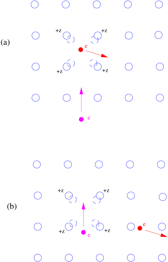
Figure 1: In (a) one electron polarizes the lattice (indicated by dashed circles displaced towards uppermost electron); in (b) that electron has moved away. In the meantime a second electron (seen below in (a)) is attracted to the polarized region, which has remained polarized long after the first electron has left the region. Figure is schematic only, and does not, for example, properly convey the opposite momenta such a pair should possess.

where $k_{\circ}$ is the Thomas-Fermi wave vector, and $\omega({\bf q})$ is the dressed phonon frequency. Eq. (1) is an effective interaction; a more formal and general approach, utilizing Green functions, will be given later. Nonetheless, it is clear that this effective interaction captures the essence of “overscreening”, i.e. for electronic energy differences less than the phonon energy, the phonon contribution to the screened interaction has the opposite sign from the electronically screened interaction, and exceeds it in magnitude. Physically [37], one electron makes a transition, which excites a phonon, accompanied by an ionic charge density fluctuation. A second electron undergoes a transition caused by this induced charge density fluctuation. If the differences in the electron energies is small compared to the phonon excitation energy, the second electron is actually attracted to the first. This is shown pictorially in Fig. 1.

Eq. (1) represents the starting point for the two-electron interaction in metals. It was further simplified for both the Cooper pair calculation [38] and the Bardeen-Cooper-Schrieffer (BCS) [5] calculation. The progression of events that ultimately led to a successful theory for BCS has been well documented [22]. Most of this part of the story had little to do with the details of the attractive mechanism, but rather with the pairing theory itself. Thus, one can divide the theory of superconductivity into two separate conquests: first the establishment of a pairing formalism, which leads to a superconducting condensate, given some attractive particle-particle interaction, and secondly, a mechanism by which two electrons might attract one another. BCS, by simplifying the interaction, succeeded in establishing the pairing formalism. They were able to explain quite a number of experiments, previously performed, in progress at the time of the formulation of the theory, and many that were to follow. However, one might well ask to what extent the experiments support the electron-phonon mechanism as being responsible for superconductivity [39]. Indeed, one of the elegant outcomes of the BCS pairing formalism is the universality of various properties; at the same time this universality means that the theory really doesn’t distinguish one superconductor from another, and, more seriously, one mechanism from another. Fortunately, while many superconductors do display universality, some do not, and these, as it turns out, provided very strong support for the electron-phonon mechanism, as initially motivated by Fröhlich [26] and by Bardeen and Pines [35]. Much of this chapter will be concerned with these deviations from universality.

After the BCS paper appeared, several workers rederived their results using alternative formalisms. For example, Anderson used an RPA treatment of the reduced BCS Hamiltonian in terms of pseudospin operators [40], and Bogoliubov and others [41, 42] developed more general methods, later to be adapted to inhomogeneous superconductivity by de Gennes [43]. Finally, Gor’kov [44] developed a Green function method, from which both the BCS results, and the Ginzburg-Landau phenomenology [45] could be derived, near the transition temperature, $T_{c}$.

The Gor’kov formalism proved to be the most useful, for the purposes of generalizing BCS theory (with its model effective interaction) to the case where the electron-phonon interaction is properly taken into account in the superconducting state. This was done by Eliashberg [1], as well as Nambu [2], and later partially by Morel and Anderson [3] and more completely by Schrieffer and coworkers [4, 46, 47]. Around the same time tunneling became a very useful spectroscopic probe of the superconducting state [48]; besides providing an excellent measure of the gap in a superconductor, it also revealed the fine detail of the electron-phonon interaction [49], to such an extent that tunneling data could be “inverted” to tell us about the underlying electron-phonon interactions [50]. These developments have been well documented in the Parks treatise [51]. In particular retardation effects are covered in the articles by Scalapino [14] and McMillan and Rowell [52]. An interesting historical perspective is provided in the article by Anderson [53].

In the meantime, developments in our understanding of the polaron were occurring in parallel. The problem of phonon-mediated superconductivity and the problem of the impact of electron-phonon interactions on a single electron are obviously related, but, after the initial work by Fröhlich and Pines and coworkers, the two fields seem to have parted ways. Indeed, an excellent summary of the status of polarons at that time is Ref. [54], where, however, there is essentially no “cross-talk” with the theory of superconductivity. Similarly, in the treatise by Parks [51] there is essentially no discussion of polarons [55], in spite of the fact that the ‘polaron’ really is the essential building block of the BCS theory of superconductivity. So, for example, a perusal of the index of the classic texts on superconductivity, by Schrieffer [46], Blatt [56], Rickayzen [57], de Gennes [43], and Tinkham [58] reveals not a single entry [59]. The reason for this is that the electron-phonon coupling strength in all known superconductors was deemed to be sufficiently weak that the only effect on normal state properties was a slightly increased electron effective mass. Thus, the electronic state is presumed to be well described by Fermi Liquid Theory, upon which the BCS theory (and its modifications) is based. It is important to keep this in mind; for this reason we will refrain from referring to Eliashberg theory as a strong coupling theory (we ourselves have used this term in the past). Eliashberg theory goes beyond BCS theory because it includes retardation effects; however, it is still a weak coupling theory, in the sense that the Fermi energy is the dominant energy, and the quasiparticle picture remains intact.

We make this distinction because in recent years polaron theory has experienced a renaissance, and some attempts to explain high temperature superconductivity have utilized polaron and bipolaron concepts. The bipolaron is simply a bound state of two polarons, analogous to the Cooper pair, except that the latter requires a Fermi sea to exist (at least in three dimensions) whereas the former exists as a tightly bound pair in the absence of a Fermi sea. In this respect bipolaron theories resemble the quasichemical theory advocated by Schafroth and coworkers [60, 56] in the 1950’s. Tightly bound electron pairs are now recognized as the strong coupling limit of the BCS ground state; the transition to the normal state is, however, governed by very different (and as yet undetermined) excitations compared to BCS theory. We will refer to some of this work in the course of this chapter.

To complete this brief historical tour, we should add that in 1964, with the suggestion of a theorist [61], what has emerged as a new class of superconductors was discovered [62]. The actual superconducting compound was doped Strontium Titanate (SrTiO₃), a perovskite with low carrier density. This compound, along with BaPb_0.75Bi_0.25O₃, another doped perovskite discovered in 1975 [63] with a transition temperature of 12 K, were the precursors to the modern high temperature superconductors discovered by Bednorz and Müller [8]. In fact, with fortuitous foresight, Schooley et al. [64] remarked, “If SrTiO₃ had magnetic properties, a complete study of this material would require a thorough knowledge of all of solid state physics.” Little did they know that in 1986 perovskites would be discovered, that not only had high superconducting transition temperatures, but also exhibited a plethora of magnetic phenomena. We should also note that the so-called cuprates, which presently exhibit superconducting transition temperatures up to 160 K (under pressure), all contain CuO₂ layers, whereas the cubic oxides (such as SrTiO₃, BaPb_0.75Bi_0.25O₃, and Ba_1-xK_xBiO₃    [65] (with $T_{c}\approx 30$ K)) do not. For this reason many workers have come to regard the layered cuprates and the cubic oxides as belonging to two completely separate (and unconventional) classes, even though they are both essentially low carrier density perovskites.

2.2 Electron-Ion Interaction

2.2.1 Overview

A useful ab initio theory has to begin from some fundamental starting point. In condensed matter systems the starting point is usually taken to be electrons and ions (with their charges, and masses, etc.) along with the chemical composition of the material [12]. Given these ingredients, the prescription for calculation is, in principle, straightforward. One has to solve the many-body Schrodinger equation, with a Hamiltonian consisting of one-body kinetic energy terms and the two-body Coulomb interaction. The form of these terms, along with all the constants involved, are known, so all that is required to solve the problem is perhaps some ingenuity along with unlimited computer resources. This has been referred to by Laughlin as the Condensed Matter version of “The Theory of Everything” [66].

Of course the difficulty is that, even if one could solve this problem, one would not recognize what the solution represented. The notion of ionic collective modes (i.e. phonons), for example, would not be very transparent in such an approach. More obscure still would be the distinction between a superconducting state versus a metallic state.

Instead, an approach which separates the complex many-body problem into smaller, more tractable pieces, has traditionally been adopted in condensed matter, and in particular in the problem of superconductivity [5, 14, 12]. The most systematic approach has been discussed by Rainer [12]. The premise in this approach is the observation that many metals (amongst which many undergo a transition to a superconducting state) are well described by Landau Fermi Liquid Theory. This allows for an asymptotic expansion in small parameters like $k_{B}T_{c}/E_{F}$, $\hbar\omega_{\rm phon}/E_{F}$ and $1/k_{F}\ell$, where $E_{F}$ ($k_{F}$) is the Fermi energy (wavevector), $\omega_{\rm phon}$ is a typical phonon frequency, and $\ell$ is the electron mean free path. He separates the problem into the “high energy problem” (effect of Coulomb interactions amongst the electrons themselves as well as between the electrons and the fixed nuclear potentials), and the “low energy problem” (the dressing of conduction electrons with phonons), and the eventual formation of the superconducting state. Most of this review will concern the low energy problem. In our opinion the high energy problem is not at all solved at present, from a truly “ab initio” approach. For example, strictly speaking, one cannot rely on any of the expansion parameters mentioned above, because one does not know, in principle, whether one has a metal with a well-defined Fermi surface, to begin with. Nonetheless, by appealing to experimental observation, one can use for many cases the fact that nature has already solved the high energy problem, and proceed from there to solve the low energy part. This has been the dominant philosophy throughout most of the last four decades towards understanding superconductivity.

The difficulty with this approach was exemplified by the discovery of superconductivity in the layered perovskites; band structure calculations for the parent compound (La₂CuO₄) demonstrated that it was a metal, when in fact the real material was an antiferromagnetic insulator. This problem was later repaired [67], but it remains the case that band structure calculations fail to properly take into account strong Coulomb correlations, and remain somewhat powerless to reliably predict a breakdown of the Fermi Liquid picture.

With these caveats, the “ab initio” approach of Ref. [12] has experienced excellent success in cases where a metallic state is known to exist, and experimental input has been used in the theory. We will comment in particular on the “low energy” part of the theory later in this chapter. A thorough discussion is available in Ref. [12].

2.2.2 Models

The net result of a proper handling of the “high energy” problem in the case of a well-behaved metal is a set of input parameters for the low energy problem that are simple enough to make the remaining part of the problem appear to have arisen from a non-interacting model. The distinction is that the input parameters (band structure, phonon spectrum, etc.) come not directly from specified model parameters, but rather from previous calculation and/or experiment. For this reason, we now discuss possible models for the electron-phonon interaction, which, for the moment, we view as fundamental models in their own right, and not as models which somehow parameterize (and disguise) the “high energy problem”.

The reason for this is that we hope to accomplish several tasks simultaneously. First, we will in effect work through the “low energy problem” discussed in the previous subsection. Secondly, we will touch upon some of the more recent work on electron-phonon Hamiltonians, which are characterized not so much by comparison with experiment as comparison with some “exact” solution, as attained, for example, by Quantum Monte Carlo methods [68, 69]. Thirdly, we will also be able to make contact with recent ongoing work on the polaron (and bipolaron). These latter two topics are presented here more by way of a digression. Some further detail is presented in an Appendix, but for a more thorough discussion the cited literature will have to be consulted.

It is always tempting to immediately compare the results of a calculation with experiment; agreement justifies the starting model (in this context this would mean the Hamiltonian, with associated parameters), whereas disagreement would tend to rule out the starting model as a candidate. In the many-body problem, however, life is not so simple. For one thing, we know the starting Hamiltonian, as emphasized in the previous subsection. We will get agreement with experiment if we were only able to routinely calculate any observable. However, in our endeavour to understand many-body systems, we have grown to utilize effective Hamiltonians, which would capture the essence of the phenomenon under investigation. The purpose of this strategy is twofold; we make sense of the many-body system in terms we can understand, and we make the calculation itself more tractable in practice.

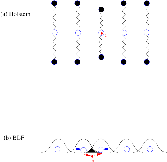
Figure 2: Schematic of ionic displacements in (a) the Holstein model, and (b) the BLF model. In (a) neighbouring chains are distorted in the vicinity of the electron, and in (b) neighbouring ions, when displaced while undergoing oscillations, lead to an increased (or decreased) overlap region (shaded in black), which leads to an altered hopping amplitude for the electron.

There are many Hamiltonians in condensed matter physics, which were derived as effective Hamiltonians for some particular problem, but, which have since taken on a life of their own. This is true because (a) they have withstood solution in spite of their simplicity, and (b) they epitomize some qualitative aspect of the more general problem. Famous examples are the Heisenberg/Ising model for spins, and the Hubbard model for fermions with spin degrees of freedom. In the electron-phonon problem several effective models have arisen over the years, the three most prominent of which have been the Fröhlich Hamiltonian [26], the Holstein model [34], and the BLF (Barišić-Labbé-Friedel) model [70] (also known as the SSH (Su-Schrieffer-Heeger) model [71]). The Fröhlich Hamiltonian was derived in a continuum approximation (see Ref. [72] or [73] for a derivation), and results in a coupling between the electron density and the ionic momentum (a canonical transformation changes this to the ionic displacement) which diverges as the momentum transfer between electron and ions goes to zero. This Hamiltonian has been the subject of many investigations of the polaron. Holstein proposed his model as a simplification in which the interaction between electron and ion is more local; in fact in some ways the simplification Hubbard [74] invoked to replace the long-range Coulomb interaction is analogous to the simplification that the Holstein model represents compared to the Fröhlich Hamiltonian. Both the Fröhlich and Holstein models represent couplings of the electron to an optical phonon mode. We will focus on the Holstein model since it is particularly amenable to numerical simulations. In contrast, the BLF (SSH) model couples the electron to the relative displacement of nearby ions, i.e. an acoustic phonon mode. The physics is simple; in the Holstein model ionic distortions affect the electron energy level at a particular site, while in the BLF model ionic displacements affect the electron hopping amplitude. These are represented pictorially in Fig. 2, although of course the coupling is dynamic.

The BLF model gained prominence in the 1980’s [75] when it was used to describe solitons in conducting polymers; otherwise comparatively little effort has been expended towards an understanding of its properties, particularly in two or three dimensions. The BLF Hamiltonian is

$$H = \sum_{i}{{\bf p}^{2}_{i}\over 2M}\phantom{aa}+\phantom{aa}\sum_{<ij>}{1\over 2}K\bigl{(}{\bf u}_{i}-{\bf u}_{j}\bigr{)}^{2}$$ (2)

$$-\sum_{<ij>\atop\sigma}\bigl{(}t_{ij}-{\bf\alpha}\cdot({\bf u}_{i}-{\bf u}_{j})\bigl{(}c^{\dagger}_{i\sigma}c_{j\sigma}\phantom{a}+\phantom{a}h.c.\bigr{)},$$

where the first line refers to the ions, with mass $M$ and spring constant $K$. The ionic degrees of freedom are described by the ion momentum, ${\bf p}_{i}$, and displacement, ${\bf u}_{i}$, at site $i$. The electrons are described by creation (annihilation) operators $c^{\dagger}_{i\sigma}$ ($c_{i\sigma}$) for an electron with spin $\sigma$ at site $i$. The electron hopping amplitude is given by $t_{ij}$; this in turn is modulated by ionic vibrations, and therefore results in the electron-ion coupling with strength $|{\bf\alpha}|$. The coupling constant $|{\bf\alpha}|$ is proportional to the gradient of the hopping overlap integral between electron orbitals on two neighbouring sites.

Equation 2 gives rise to the standard electron-phonon Hamiltonian, as written in momentum space:

$$H=\sum_{{\bf k}\sigma}\epsilon_{\bf k}c^{\dagger}_{{\bf k}\sigma}c_{{\bf k}\sigma}\phantom{a}+\phantom{a}\sum_{\bf q}\hbar\omega_{\bf q}a^{\dagger}_{\bf q}a_{\bf q}\phantom{a}+\phantom{a}{1\over\sqrt{N}}\sum_{{\bf k}{\bf k}^{\prime}\atop\sigma}g({\bf k},{\bf k}^{\prime})\bigl{(}a_{{\bf k}-{\bf k}^{\prime}}+a^{\dagger}_{-({\bf k}-{\bf k}^{\prime})}\bigr{)}c^{\dagger}_{{\bf k}^{\prime}\sigma}c_{{\bf k}\sigma}.$$ (3)

We have used the conventional oscillator operators, $a_{\bf q}={M\omega_{\bf q}\over 2\hbar}\bigl{(}{\bf u}_{\bf q}+i{\bf p}_{\bf q}\bigr{)}$ and the standard Fourier expansions, $c^{\dagger}_{i\sigma}={1\over\sqrt{N}}\sum_{\bf k}e^{i{\bf k}\cdot{\bf R}_{i}}c^{\dagger}_{{\bf k}\sigma}$, etc. The phonon dispersion is given by $\omega_{\bf q}$, where, in principle, ${\bf q}$ includes branch indices as well as momenta within the first Brillouin zone, and $g({\bf k},{\bf k}^{\prime})$ is the coupling function. For the BLF Hamiltonian, this coupling function has a very specific form (involving sine functions). A more general consideration of the electron-ion interaction yields a Hamiltonian of essentially the same form [14, 13], but where the parameters involved are understood to already contain the “high energy” effects alluded to earlier. State-of-the-art computations of the electron-ion coupling strength, are given, for example, in Ref. [76] (for La_2-xSr_xCuO₄) and in Ref. [77] (and references therein, for A₃C₆₀).

The Holstein Hamiltonian is

$$H=-t\sum_{{<ij>}\atop\sigma}(c^{\dagger}_{i\sigma}c_{j\sigma}+H.c.)+\sum_{i}[{p^{2}_{i}\over 2M}+{1\over 2}K{x}^{2}_{i}]-\alpha\sum_{i\sigma}x_{i}n_{i\sigma},$$ (4)

where the parameters are as before except that the displacement variable $x_{i}$ represents the (one-dimensional) displacement of some optical mode (say a breathing mode) associated with the $i$th site, and the electron-ion coupling $\alpha$ represents the change in site energy (per unit displacement) associated with this mode. In momentum space this Hamiltonian is particularly simple:

$$H=\sum_{{\bf k}\sigma}\epsilon_{\bf k}c^{\dagger}_{{\bf k}\sigma}c_{{\bf k}\sigma}\phantom{a}+\phantom{a}\sum_{\bf q}\hbar\omega_{E}a^{\dagger}_{\bf q}a_{\bf q}\phantom{a}+\phantom{a}{g\over\sqrt{N}}\sum_{{\bf k}{\bf q}\atop\sigma}\bigl{(}a_{\bf q}+a^{\dagger}_{-(\bf q)}\bigr{)}c^{\dagger}_{{\bf k+q}\sigma}c_{{\bf k}\sigma},$$ (5)

where $\omega_{E}$ is the Einstein mode frequency and $g\equiv\sqrt{{\alpha^{2}\hbar\omega_{E}\over 2K}}$. This model has been studied extensively in the last twenty years, at least partly due to its simplicity. Some of this work is reviewed in the Appendix.

2.3 Migdal Theory

The primary language of many-body systems is the Green function, or propagator. Many books have been written (see for example Refs. [78, 79, 80, 81, 82, 83]) about the Green function formalism, so we will bypass a thorough discussion here. A sketch of the derivation of the Migdal [84] equation for the electron self-energy is given in the Appendix. Migdal argued that all vertex corrections are $O(m/M)^{1/2}$ compared to the bare vertex, and therefore can be ignored. Here $m$ ($M$) is the electron (ion) mass. This represents a tremendous simplification, and allows one to solve a theory which should work for arbitrary coupling strength (this is, in fact, not the case, for reasons that will become apparent in the next section).

An “exact” formulation of the electron-phonon problem can be summarized [84, 85, 86] in terms of the Dyson equations (written in momentum and imaginary frequency space):

$$G({\bf k},i\omega_{m})=\bigl{[}G_{\circ}({\bf k},i\omega_{m})^{-1}-\Sigma({\bf k},i\omega_{m})\bigr{]}^{-1}$$ (6)

for the electron, and

$$D({\bf q},i\nu_{n})=\bigl{[}D_{\circ}({\bf q},i\nu_{n})^{-1}-\Pi({\bf q},i\nu_{n})\bigr{]}^{-1}$$ (7)

for the phonon, where $G({\bf k},i\omega_{m})$ is the one-electron Green function, $D({\bf q},i\nu_{n})$ is the phonon propagator, and $\Sigma({\bf k},i\omega_{m})$ is the electron and $\Pi({\bf q},i\nu_{n})$ the phonon self energy. Then,

$$\Sigma({\bf k},i\omega_{m})=-{1\over N\beta}\sum_{{\bf k^{\prime}},m^{\prime}}g_{\bf k,k^{\prime}}D({\bf k-k^{\prime}},i\omega_{m}-i\omega_{m^{\prime}})G({\bf k^{\prime}},i\omega_{m^{\prime}})\Gamma({\bf k^{\prime}},i\omega_{m^{\prime}};{\bf k},i\omega_{m};{\bf k-k^{\prime}},i\omega_{m}-i\omega_{m^{\prime}}),$$ (8)

and

$$\Pi({\bf q},i\nu_{n})={2\over N\beta}\sum_{{\bf k},m}g_{\bf k,k+q}G({\bf k+q},i\omega_{m}+i\nu_{n})G({\bf k},i\omega_{m})\Gamma({\bf k+q},i\omega_{m}+i\nu_{n};{\bf k},i\omega_{m};{\bf q},i\nu_{n}),$$ (9)

where the vertex function $\Gamma$ can only be defined in terms of an infinite set of diagrams (i.e. not in closed form).

The non-interacting propagators are

$$G_{\circ}({\bf k},i\omega_{m})=\bigl{[}i\omega_{m}-(\epsilon_{\bf k}-\mu)\bigr{]}^{-1}$$ (10)

for the electron and

$$D_{\circ}({\bf q},i\nu_{n})=\bigl{[}-M(\omega^{2}({\bf q})+\nu_{n}^{2})\bigr{]}^{-1}$$ (11)

for the phonon, where $\epsilon_{\bf k}$ is the single electron dispersion (band indices are implicit here and in the following), $\mu$ is the chemical potential, and $\omega({\bf q})$ is the phonon dispersion. In writing these relations we have adopted the finite temperature Matsubara formalism, with Fermion ($i\omega_{m}\equiv i\pi T(2m-1)$) and Boson ($i\nu_{n}\equiv i2\pi Tn$) Matsubara frequencies, where $m$ and $n$ are integers and $T$ is the temperature ($k_{B}\equiv 1$). The Matsubara sums in Eqs. (8,9) extend over all integers, and the momentum sums extend over the first Brillouin zone. This convention will be maintained unless noted otherwise.

Migdal’s approximation was to set the vertex function $\Gamma$ equal to the bare vertex, $g$. Then, the electron self-energy can be written:

$$\Sigma({\bf k},i\omega_{m})=-{1\over N\beta}\sum_{{\bf k^{\prime}},m^{\prime}}|g_{\bf k,k^{\prime}}|^{2}D({\bf k-k^{\prime}},i\omega_{m}-i\omega_{m^{\prime}})G({\bf k^{\prime}},i\omega_{m^{\prime}}).$$ (12)

Migdal [84] also included renormalization effects in the phonon propagator. With an application to real materials in mind, however, the electron dispersion relations will have been obtained from a band structure calculation, and the phonon properties will generally have been taken from experiment. In this case the phonon self energy is omitted entirely (to avoid double counting). In addition electron-electron effects have been omitted, as they have been presumed to be included already in the band structure and phonon calculations (to the best extent possible).

Alternatively, Eq. (12) can be viewed as having been derived from some microscopic electron-ion Hamiltonian. For example, in the case of the Holstein Hamiltonian, Eq. (4), $g_{\bf k,k^{\prime}}\rightarrow g$, the constant appearing in Eq. (5), and the electron band structure is given by $\epsilon_{\bf k}=-2t\cos{(k_{x})}$ (in one dimension, and for nearest-neighbour hopping only). In addition, the phonon frequency becomes dispersionless ($\omega({\bf q})\rightarrow\omega_{E}$) and the phonon self energy is given by some appropriate approximation. Such an identification is useful for comparison to exact results (usually done numerically - see the Appendix for references).

In the classical literature [84, 85, 87, 88, 13], Eq. (12) is simplified in the following way. First, very often the phonon propagator is provided separately, usually by inelastic neutron scattering measurements [89, 90]. To see how, one first writes the phonon propagator in terms of its spectral representation [13]:

$$D({\bf q},i\nu_{n})=\int_{0}^{\infty}d\nu B({\bf q},\nu){2\nu\over(i\nu_{n})^{2}-\nu^{2}}$$ (13)

where $B({\bf q},\nu)$ is the phonon spectral function

$$B({\bf q},\nu)\equiv-{1\over\pi}{\rm Im}D({\bf q},\nu+i\delta).$$ (14)

The spectral function is positive definite, and obeys a sum rule; it is the quantity that is constructed with fits to high-symmetry phonon dispersion curves measured by inelastic neutron scattering [89]. Following this tact a calculation of the phonon self energy is no longer required. Another simplification was recognized in Ref. [85]; this is the use of the non-interacting electron Green function $G_{\circ}({\bf k},i\omega_{m})$ in the right hand side of Eq. (12) instead of the full self-consistent choice, $G({\bf k},i\omega_{m})$. This approximation is valid when particle-hole symmetry is present and the infinite bandwidth approximation is invoked. This latter approximation is used extensively in the early literature on metals and superconductors; a systematic explanation of the logic is provided in Ref. [13], and requires the usual hierarchy of energy scales, $\omega_{\rm phon}<<E_{F}$ ($\hbar\equiv 1$). The result is

$$\Sigma({\bf k},i\omega_{m})={1\over N\beta}\sum_{{\bf k^{\prime}},m^{\prime}}\int_{0}^{\infty}d\nu|g_{\bf k,k^{\prime}}|^{2}B({\bf k-k^{\prime}},\nu){2\nu\over(\omega_{m}-\omega_{m^{\prime}})^{2}+\nu^{2}}G_{\circ}({\bf k^{\prime}},i\omega_{m^{\prime}}).$$ (15)

The form of Eq. (15) allows one to introduce the electron-phonon spectral function,

$$\alpha^{2}F({\bf k,k^{\prime}},\nu)\equiv N(\mu)|g_{\bf k,k^{\prime}}|^{2}B({\bf k-k^{\prime}},\nu),$$ (16)

where $N(\mu)$ is the electron density of states at the chemical potential. At this point one can introduce ‘Fermi surface Harmonics’ [91, 13], and define an electron self-energy with Fermi momentum which depends on Matsubara frequency, and on the angle around the Fermi surface. Elastic impurities would act to homogenize the self-energy (as well as other properties), so a more useful function for dirty superconductors is the Fermi-surface-averaged spectral function,

$$\alpha^{2}F(\nu)\equiv{1\over N(\mu)^{2}}\sum_{\bf k,k^{\prime}}\alpha^{2}F({\bf k,k^{\prime}},\nu)\delta(\epsilon_{\bf k}-\mu)\delta(\epsilon_{\bf k^{\prime}}-\mu).$$ (17)

To gain an understanding of electron-phonon effects, Englesberg and Schrieffer [85] solved this model for two simple phonon models, the Einstein and Debye models. Here we summarize their results for the Einstein model, with unmodified phonon spectrum, a simpler case since both the phonon spectrum and the bare vertex function are independent of momentum. In this case $g_{\bf k,k^{\prime}}\equiv g$ and $B({\bf q},\nu)\equiv\delta(\nu-\omega_{E})$. Using, in addition, the prescription

$${1\over N}\sum_{\bf k}\rightarrow\int d\epsilon N(\epsilon)$$ (18)

along with a constant density of states approximation, extended over an infinite bandwidth, one obtains for the electron self energy

$$\Sigma(i\omega_{m})=\lambda\omega_{E}^{2}\int_{-\infty}^{\infty}d\epsilon\,{1\over\beta}\sum_{m^{\prime}}{1\over\omega_{E}^{2}+(\omega_{m^{\prime}}-\omega_{m})^{2}}{1\over i\omega_{m^{\prime}}-(\epsilon-\mu)},$$ (19)

where we have used the standard definition for the electron-phonon mass enhancement parameter, $\lambda$:

$$\lambda\equiv 2\int_{0}^{\infty}d\nu{\alpha^{2}F(\nu)\over\nu},$$ (20)

which, for the Einstein spectrum used here, reduces to

$$\lambda=2N(\epsilon_{F})g^{2}/\omega_{E}.$$ (21)

Performing the Matsubara sum yields

$$\Sigma(i\omega_{m})={\lambda\omega_{E}\over 2}\int_{-\infty}^{\infty}d\epsilon\biggl{(}\,\,{n(\omega_{E})+1-f(\epsilon-\mu)\over i\omega_{m}-\omega_{E}-(\epsilon-\mu)}+{n(\omega_{E})+f(\epsilon-\mu)\over i\omega_{m}+\omega_{E}-(\epsilon-\mu)}\,\,\biggr{)}$$ (22)

where $f(\epsilon-\mu)$ is the Fermi function and $n(\omega_{E})$ is the Bose distribution function. The remaining integral can also be performed [13]

$$\Sigma(z)={\lambda\omega_{E}\over 2}\biggl{[}\,\,-2\pi i(n(\omega_{E})+1/2)+\psi\bigl{(}{1\over 2}+i{\omega_{E}-z\over 2\pi T}\bigr{)}-\psi\bigl{(}{1\over 2}-i{\omega_{E}+z\over 2\pi T}\bigr{)}\,\,\biggr{]}$$ (23)

where $\psi(x)$ is the digamma function [92, 13] and the entire expression has been analytically continued to a general complex frequency $z$. Because we performed the Matsubara sum first, before replacing $i\omega_{m}$ with $z$, this is the physically correct analytic continuation [93].

At zero temperature one can use well-documented properties of the digamma function, or, more simply, refer to the analytic continuation of Eq. (22), since the Bose and Fermi functions may be more familiar. Since $n(\omega_{E})\rightarrow 0$ and $f(\epsilon-\mu)\rightarrow\theta(\mu-\epsilon)$ as $T\rightarrow 0$ ($\theta(x)$ is the Heaviside step function), the self energy at $T=0$ is

$$\Sigma(z)={\lambda\omega_{E}\over 2}\ln\biggl{(}{\omega_{E}-z\over\omega_{E}+z}\biggr{)}.$$ (24)

Spectroscopic measurements yield properties as a function of real frequency; because of the analytic properties of the Green function, this corresponds to a frequency either slightly above or below the real axis. We will use frequencies slightly above, and designate the infinitesmal positive imaginary part by ‘$i\delta$’. Thus,

$$\Sigma(\omega+i\delta)={\lambda\omega_{E}\over 2}\Biggl{[}\ln\mid{\omega_{E}-\omega\over\omega_{E}+\omega}\mid-i\pi\theta(\mid\omega\mid-\omega_{E})\Biggr{]}.$$ (25)

The real and imaginary parts of this self energy are shown in Fig. 3, along with the non-interacting inverse Green function ($\omega-(\epsilon_{\bf k}-\mu)$) to determine the poles of the electron Green function (see Eq. (6)) graphically. A quantity often measured in single particle spectroscopies is the spectral function, $A({\bf k},\omega)$ defined by

$$A({\bf k},\omega)\equiv-{1\over\pi}{\rm Im}G({\bf k},\omega+i\delta).$$ (26)

With this definition, we obtain, through Eq. (6) and (25),

$$A({\bf k},\omega) = \delta\biggl{(}\omega-(\epsilon_{\bf k}-\mu)-{\lambda\omega_{E}\over 2}\ln\mid{\omega_{E}-\omega\over\omega_{E}+\omega}\mid\biggr{)}\phantom{aaaaaaaaaa}{\rm if}\mid\omega\mid<\omega_{E},$$ (27)

$$= {\lambda\omega_{E}/2\over\biggl{(}\omega-(\epsilon_{\bf k}-\mu)-{\lambda\omega_{E}\over 2}\ln\mid{\omega_{E}-\omega\over\omega_{E}+\omega}\mid\biggr{)}^{2}\,+\,\biggl{(}{\pi\lambda\omega_{E}\over 2}\biggr{)}^{2}}\phantom{aaa}{\rm if}\mid\omega\mid>\omega_{E}.$$

Plots are shown in Fig. 4. Each spectral function displays a quasiparticle peak, whose strength $a_{\bf k}$ and frequency $\omega_{\bf k}$ is implicitly dependent on wavevector

$$a_{\bf k}=\biggl{(}1+{\lambda\over 1-(\omega_{\bf k}/\omega_{E})^{2}}\biggr{)}^{-1},$$ (28)

where $\omega_{\bf k}$ is the solution (between $-\omega_{E}$ and $\omega_{E}$) to the zero of the delta-function argument in Eq. (27). For all momenta (or equivalently all $\epsilon_{\bf k}-\mu$) there is a solution, whose frequency approaches $\omega_{E}$ asymtotically as $\epsilon_{\bf k}-\mu\rightarrow\infty$. The weight of this peak starts at the Fermi surface ($\epsilon_{\bf k}=\mu$) as $1/(1+\lambda)$ and quickly goes to zero according to Eq. (28) as $\omega_{\bf k}\rightarrow\omega_{E}$, which occurs for $\epsilon_{\bf k}{>\atop\sim}2\omega_{E}$. For larger $\epsilon_{\bf k}$ a quasiparticle peak forms once again, albeit with non-zero width, at approximately the non-interacting electron energy, $\epsilon_{\bf k}=\mu$. At intermediate $\epsilon_{\bf k}\approx\omega_{E}$, the quasiparticle picture has broken down, and a description as described here is required for a complete picture.

How well the Migdal approximation works in specific circumstances is the subject of ongoing research (see, for example, Refs. [94, 95, 96, 97, 98], and the Appendix. For example, Alexandrov et al. [99] found an apparent breakdown (for coupling strengths greater than 1, within the Holstein model) to the approximation when a finite electronic bandwidth was taken into account.

We have focussed on the modifications to the electron spectral function due to the electron-phonon interaction. For excitations at the Fermi level ($\epsilon_{\bf k}=\mu$), the quasiparticle pole remains there ($\omega_{\bf k_{F}}=0$), remains infinitely long-lived (it is a delta-function), but has a reduced weight, by a factor of $1+\lambda$. This same factor enhances the effective mass, and alters various normal state properties in a similar way [100, 88]. For example, the low temperature electronic specific heat is linear in temperature with coefficient usually denoted by $\gamma$, which is proportional to the electron density of states. The electron-phonon interaction enhances this coefficient by the same factor, $1+\lambda$. Other renormalizations are reviewed in Ref. [88].

2.4 Eliashberg Theory

Eliashberg theory is the natural development of BCS theory to include retardation effects due to the ‘sluggishness’ of the phonon response. In fact, insofar as BCS introduced an energy cutoff, $\omega_{D}$ (the Debye frequency), they included, in the most minimal way, retardation effects. However, Eliashberg theory goes well beyond this approximation, and handles momentum cutoffs and frequency cutoffs separately. We begin this section with a very brief review of BCS theory, followed by a more detailed discussion of Eliashberg theory.

2.4.1 BCS Theory

Before one establishes a theory of superconductivity, one requires a satisfactory theory of the normal state. In conventional superconductors, Fermi Liquid Theory appears to work very well, so that, while we cannot solve the problem of electrons interacting through the Coulomb interaction, experiment tells us that Coulomb interactions give rise to well-defined quasiparticles, i.e. a set of excitations which are in one-to-one correspondence with those of the free-electron gas. The net result is that one begins the problem with a ‘reduced’ Hamiltonian,

$$H_{\rm red}=\sum_{{\bf k}\sigma}\epsilon_{\bf k}c^{\dagger}_{{\bf k}\sigma}c_{{\bf k}\sigma}\phantom{a}+\phantom{a}\sum_{{\bf k}{\bf k}^{\prime}}V_{{\bf k},{\bf k}^{\prime}}c^{\dagger}_{{\bf k}\uparrow}c^{\dagger}_{-{\bf k}\downarrow}c_{-{\bf k}^{\prime}\downarrow}c_{{\bf k}\uparrow},$$ (29)

where, for example, the electron energy dispersion $\epsilon_{\bf k}$ already contains much of the effect due to Coulomb interactions. The important point is that well-defined quasiparticles with a well-defined energy dispersion near the Fermi surface are assumed to exist, and are summarized by the dispersion $\epsilon_{\bf k}$. The pairing interaction $V({\bf k},{\bf k}^{\prime})$ is assumed to be ‘left-over’ from the main part of the Coulomb interaction, and this is the part that BCS simply modelled, based on earlier work by Fröhlich [26] and Bardeen and Pines [35].

Complete derivations of BCS theory have been provided elsewhere in this volume; here we state the final result [46]:

$$\Delta_{\bf k}=-{1\over N}\sum_{\bf k^{\prime}}V_{{\bf k},{\bf k}^{\prime}}{\Delta_{\bf k^{\prime}}\over 2E_{\bf k^{\prime}}}\tanh{\beta E_{\bf k^{\prime}}\over 2},$$ (30)

where

$$E_{\bf k}=\sqrt{(\epsilon_{\bf k}-\mu)^{2}+\Delta_{\bf k}^{2}}$$ (31)

is the quasiparticle energy in the superconducting state, and $\Delta_{\bf k}$ is the variational parameter used by BCS. An additional equation which must be considered alongside the gap equation (30) is the number equation,

$$n=1-{1\over N}\sum_{{\bf k}}{\epsilon_{{\bf k}}-\mu\over E_{{\bf k}}}\tanh{\beta E_{\bf k}\over 2}.$$ (32)

Given a pair potential and an electron density, one has to ‘invert’ these equations to determine the variational parameter $\Delta_{\bf k}$ and the chemical potential. For conventional superconductors the chemical potential hardly changes on going from the normal to the superconducting state, and the variational parameter is much smaller than the chemical potential, with the result that the second equation was usually ignored.

BCS then modelled the pairing interaction as a negative (and therefore attractive) constant with a sharp cutoff in momentum space:

$$V_{{\bf k},{\bf k}^{\prime}}\approx-V\theta(\omega_{D}-\mid(\epsilon_{\bf k}-\mu)\mid)\theta(\omega_{D}-\mid(\epsilon_{\bf k^{\prime}}-\mu)\mid).$$ (33)

Using this potential in Eq. (30), along with a constant density of states assumption over the entire range of integration, we obtain

$${1\over\lambda}=\int_{0}^{\omega_{D}}{d\epsilon\over E}\,\tanh{\beta E\over 2},$$ (34)

where $\lambda\equiv N(\mu)V$. At $T=0$, the integral can be done analytically to give

$$\Delta=2\omega_{D}{\exp{(-1/\lambda)}\over 1-\exp{(-1/\lambda)}}.$$ (35)

In weak coupling this becomes the more familiar

$$\Delta=2\omega_{D}\exp{(-1/\lambda)},$$ (36)

while in strong coupling we obtain

$$\Delta=2\omega_{D}\lambda.$$ (37)

Both of these results are within the realm of BCS theory (at zero temperature) [101, 102], although the latter generally requires a self-consistent solution with the number equation, Eq. (32).

Close to the critical temperature, $T_{c}$, the BCS equation becomes

$${1\over\lambda}=\int_{0}^{\beta\omega_{D}/2}dx\,{\tanh{x}\over x},$$ (38)

which can’t be solved in terms of elementary functions for arbitrary coupling strength. Nonetheless, in weak coupling, one obtains

$$T_{c}=1.13\omega_{D}\exp{(-1/\lambda)},$$ (39)

and in strong coupling

$$T_{c}=\omega_{D}\lambda/2.$$ (40)

It is clear that $T_{c}$ or the zero temperature variational parameter $\Delta$ depend on material properties such as the phonon spectrum ($\omega_{D}$), the electronic structure ($N(\mu)$) and the electron-ion coupling strength ($V$). However, it is possible to form various thermodynamic ratios, which turn out to be independent of material parameters. The obvious example from the preceding equations is the ratio ${2\Delta\over k_{B}T_{c}}$. In weak coupling (most relevant for conventional superconductors), for example, we obtain

$${2\Delta\over k_{B}T_{c}}=3.53,$$ (41)

a universal result, independent of the material involved. Many other such ratios can be determined within BCS theory, and the observed deviations from these universal values contributed to the need for an improved formulation of BCS theory. For example, the observed value of this ratio in superconducting Pb was closer to 4.5, a result that is readily understood with Eliashberg theory. It is worth noting that simply extending BCS theory to the strong coupling limit (see Eqs. (37,40) above) results again in a universal constant, ${2\Delta\over k_{B}T_{c}}=4$, which is the maximum value attainable within BCS theory with a constant interaction [103], and is still clearly too low.

Other aspects of BCS theory, particularly those which prove to inadequately account for the superconducting properties of some materials (notably Pb and Hg) will not be reviewed here. Instead, we will make reference to the BCS limit as we encounter various properties within the experimental or Eliashberg context.

2.4.2 Eliashberg Equations

In most reviews and texts that derive the Eliashberg equations, the starting point is the Nambu formalism [2]. While this formalism simplifies the actual derivation, it also provides a roadblock to further understanding for the uninitiated. For this reason we have followed the conceptually much more straightforward approach (provided by Rickayzen [57], for example) in the derivation outlined in the Appendix. The result can be summarized by the following set of equations:

$$\Sigma({\bf k},i\omega_{m}) \equiv {1\over N\beta}\sum_{{\bf k^{\prime}},m^{\prime}}{\lambda_{{\bf k}{\bf k^{\prime}}}(i\omega_{m}-i\omega_{m^{\prime}})\over N(\mu)}G({\bf k}^{\prime},i\omega_{m^{\prime}})$$ (42)

$$\phi({\bf k},i\omega_{m}) \equiv {1\over N\beta}\sum_{{\bf k^{\prime}},m^{\prime}}\Biggl{[}{\lambda_{{\bf k}{\bf k^{\prime}}}(i\omega_{m}-i\omega_{m^{\prime}})\over N(\mu)}-V_{\bf kk^{\prime}}\Biggr{]}F({\bf k}^{\prime},i\omega_{m^{\prime}}),$$ (43)

$$G({\bf k},i\omega_{m}) = {G^{-1}_{n}({\bf k},i\omega_{m})\over G^{-1}_{n}({\bf k},i\omega_{m})G^{-1}_{n}(-{\bf k},-i\omega_{m})+\phi({\bf k},i\omega_{m})\bar{\phi}({\bf k},i\omega_{m})}$$ (44)

$$F({\bf k},i\omega_{m}) = {\phi({\bf k},i\omega_{m})\over G^{-1}_{n}({\bf k},i\omega_{m})G^{-1}_{n}(-{\bf k},-i\omega_{m})+\phi(-{\bf k},-i\omega_{m})\bar{\phi}(-{\bf k},-i\omega_{m})}$$ (45)

$$G^{-1}_{n}({\bf k},i\omega_{m}) = G^{-1}_{\circ}({\bf k},i\omega_{m})-\Sigma({\bf k},i\omega_{m}).$$ (46)

Another couple of equations identical to Eqs. (43) and (45), except with $\bar{\phi}$ and $\bar{F}$ instead of $\phi$ and $F$, have been omitted; they indicate that some choice of phase is possible, which will be important for Josephson effects [104] but not for what will be considered in the remainder of this chapter. Therefore, we use $\bar{\phi}=\phi$ [105].

Note that $G^{-1}_{\circ}({\bf k},i\omega_{m})$ is the inverse of the non-interacting Green function, in which Hartree-Fock contributions from both the electron-ion and electron-electron interactions are assumed to be contained.

Following the standard practice we have used a kernel given by

$$\lambda_{{\bf k}{\bf k^{\prime}}}(z)\equiv\int_{0}^{\infty}{2\nu\alpha_{{\bf k}{\bf k^{\prime}}}^{2}F(\nu)\over\nu^{2}-z^{2}}d\nu$$ (47)

where $\alpha_{{\bf k}{\bf k^{\prime}}}^{2}F(\nu)$ is given by Eq. (16). Eqs. (42-47) have been written in a fairly general way; in this way they can be viewed as having arisen from a microscopic Hamiltonian as in Eqs. (2-4) (although electron-electron interactions have been included in the pairing channel only, and not in the single electron self energy), or, alternatively, from a treatment of real metals, where, as mentioned earlier, the electron and phonon structure come from previous calculations and/or experiments. These equations emphasize the electron-ion interaction; attempts to explain superconductivity through the electron-electron interactions have been proposed in the past, mainly through collective modes [106, 107, 108, 109, 111, 112, 110, 113]; some of these attempts will be treated elsewhere in this volume in the context of high temperature superconductivity.

Assuming the electron and phonon structure is given, Eqs. (42-47) must be solved for the two functions, $\Sigma({\bf k},i\omega_{m})$ and $\phi({\bf k},i\omega_{m})$. The procedure is as follows: it is standard practice to separate the self energy, $\Sigma({\bf k},i\omega_{m})$, into its even and odd components [13]:

$$i\omega_{m}\bigl{[}1-Z({\bf k},i\omega_{m})\bigr{]} \equiv {1\over 2}\bigl{[}\Sigma({\bf k},i\omega_{m})-\Sigma({\bf k},-i\omega_{m})\bigr{]}$$

$$\chi({\bf k},i\omega_{m}) \equiv {1\over 2}\bigl{[}\Sigma({\bf k},i\omega_{m})+\Sigma({\bf k},-i\omega_{m})\bigr{]}$$ (48)

where $Z$ and $\chi$ are both even functions of $i\omega_{m}$ (and, as we’ve assumed all along, ${\bf k}$). Then, Eq. (42) becomes two equations,

$$Z({\bf k},i\omega_{m})=1+{1\over N\beta}\sum_{{\bf k^{\prime}},m^{\prime}}{\lambda_{{\bf k}{\bf k^{\prime}}}(i\omega_{m}-i\omega_{m^{\prime}})\over N(\mu)}{\bigl{(}\omega_{m^{\prime}}/\omega_{m}\bigr{)}Z({\bf k^{\prime}},i\omega_{m^{\prime}})\over\omega_{m^{\prime}}^{2}Z^{2}({\bf k^{\prime}},i\omega_{m^{\prime}})+\bigl{(}\epsilon_{\bf k^{\prime}}-\mu+\chi({\bf k^{\prime}},i\omega_{m^{\prime}})\bigr{)}^{2}+\phi^{2}({\bf k^{\prime}},i\omega_{m^{\prime}})}$$ (49)

$$\chi({\bf k},i\omega_{m})=-{1\over N\beta}\sum_{{\bf k^{\prime}},m^{\prime}}{\lambda_{{\bf k}{\bf k^{\prime}}}(i\omega_{m}-i\omega_{m^{\prime}})\over N(\mu)}{\epsilon_{\bf k^{\prime}}-\mu+\chi({\bf k^{\prime}},i\omega_{m^{\prime}})\over\omega_{m^{\prime}}^{2}Z^{2}({\bf k^{\prime}},i\omega_{m^{\prime}})+\bigl{(}\epsilon_{\bf k^{\prime}}-\mu+\chi({\bf k^{\prime}},i\omega_{m^{\prime}})\bigr{)}^{2}+\phi^{2}({\bf k^{\prime}},i\omega_{m^{\prime}})}$$ (50)

along with the gap equation (Eq. (43)):

$$\phi({\bf k},i\omega_{m})={1\over N\beta}\sum_{{\bf k^{\prime}},m^{\prime}}\biggl{(}{\lambda_{{\bf k}{\bf k^{\prime}}}(i\omega_{m}-i\omega_{m^{\prime}})\over N(\mu)}-V_{\bf kk^{\prime}}\biggr{)}{\phi({\bf k^{\prime}},i\omega_{m^{\prime}})\over\omega_{m^{\prime}}^{2}Z^{2}({\bf k^{\prime}},i\omega_{m^{\prime}})+\bigl{(}\epsilon_{\bf k^{\prime}}-\mu+\chi({\bf k^{\prime}},i\omega_{m^{\prime}})\bigr{)}^{2}+\phi^{2}({\bf k^{\prime}},i\omega_{m^{\prime}})}.$$ (51)

These are supplemented with the electron number equation, which determines the chemical potential, $\mu$:

$$n = {2\over N\beta}\sum_{{\bf k^{\prime}},m^{\prime}}G({\bf k^{\prime}},i\omega_{m^{\prime}})e^{i\omega_{m^{\prime}}0^{+}}$$ (52)

$$= 1-{2\over N\beta}\sum_{{\bf k^{\prime}},m^{\prime}}{\epsilon_{\bf k^{\prime}}-\mu+\chi({\bf k^{\prime}},i\omega_{m^{\prime}})\over\omega_{m^{\prime}}^{2}Z^{2}({\bf k^{\prime}},i\omega_{m^{\prime}})+\bigl{(}\epsilon_{\bf k^{\prime}}-\mu+\chi(({\bf k^{\prime}},i\omega_{m^{\prime}})\bigr{)}^{2}+\phi^{2}({\bf k^{\prime}},i\omega_{m^{\prime}})}.$$ (53)

These constitute general Eliashberg equations for the electron-phonon interaction, in which electron-electron interactions enter explicitly only in the pairing equation. Very complete calculations of these functions (linearized, for the calculation of $T_{c}$) were carried out for Nb by Peter et al. [114], and for Pb by Daams [115].

The more standard practice is to essentially confine all electronic properties to the Fermi surface; then only the anisotropy of the various functions need be considered. Often these are simply averaged over (due to impurities, for example), or the anisotropy may be very weak and therefore neglected. In this case the equations (49-53) can be written

$$Z_{m} = 1+\pi T\sum_{m^{\prime}}\lambda(i\omega_{m}-i\omega_{m^{\prime}}){(\omega_{m^{\prime}}/\omega_{m})Z_{m^{\prime}}\over\sqrt{\omega_{m^{\prime}}^{2}Z^{2}_{m^{\prime}}+\phi^{2}_{m^{\prime}}}}A_{0}(m^{\prime})$$ (54)

$$\chi_{m} = -\pi T\sum_{m^{\prime}}\lambda(i\omega_{m}-i\omega_{m^{\prime}})A_{1}(m^{\prime})$$ (55)

$$\phi_{m} = \pi T\sum_{m^{\prime}}\biggl{(}\lambda(i\omega_{m}-i\omega_{m^{\prime}})-N(\mu)V_{\rm coul}\biggr{)}{\phi_{m^{\prime}}\over\sqrt{\omega_{m^{\prime}}^{2}Z^{2}_{m^{\prime}}+\phi^{2}_{m^{\prime}}}}A_{0}(m^{\prime})$$ (56)

$$n = 1-2\pi TN(\mu)\sum_{m^{\prime}}A_{1}(m^{\prime})$$ (57)

where we have adopted the shorthand $Z(i\omega_{m})=Z_{m}$, etc, $\lambda(z)$ and $V_{\rm coul}$ represent appropriate Fermi surface averages of the quantities involved, and the functions $A_{0}(m^{\prime})$ and $A_{1}(m^{\prime})$ are given by integrals over appropriate density of states, using the prescription (18) to convert from Eqs. (49-53) to Eqs. (54-57). If the electron density of states is assumed to be constant, then, with the additional approximation of infinite bandwidth, $A_{0}(m^{\prime})\equiv 1$ (actually a cutoff, $\theta(\omega_{c}-\mid\omega_{m^{\prime}}\mid)$, is required in Eq. (56)), and $A_{1}(m^{\prime})\equiv 0$. This last result effectively removes $\chi_{m}$ (and Eqs. (55,57) ) from further consideration. An earlier review by one of us [11] covered the consequences of the remaining two coupled equations in great detail.

Nonetheless, a considerable effort has been devoted to examining gap anisotropy, as well as variations in the electronic density of states near the Fermi surface. We describe some of this work in the following few paragraphs.

Referring back to Eqs. (49-53), one can rewrite the summation over ${\bf k^{\prime}}$ on the right-hand-side of these equations as an integral over energy plus an integral over angle (for a given constant energy surface). In carrying out the energy integration the energy dependent electron density of states (EDOS), $N(\epsilon)$, introduces a new weighting factor if $N(\epsilon)$ exhibits variations over the energy scale of the phonon frequencies. On the other hand, the integration over angle will account for variations of the gap and other quantities in the integrands with momentum direction. There is a large literature on each of these complicating effects, starting with anisotropy effects [116, 117], and more recently with EDOS energy dependence [118, 119, 120, 13].

Concerning anisotropy, the observed universal decrease in $T_{c}$ with increasing impurity concentration (i.e. so-called ‘normal’ impurities, deemed to be innocuous by Anderson’s argument [121]) can be attributed to the washing out of gap anisotropy. To see why this decreases $T_{c}$ (we omit here effects due to valence changes) we note that the impurity potential scattering has a tendency to homogenize the gap on the Fermi surface. This tends to reduce the gap in some directions, and it is these directions that make the maximum contribution to $T_{c}$, and so $T_{c}$ is reduced. A simple BCS calculation can demonstrate this analytically. One makes a separable approximation for the pairing potential, Eq. (33), to be used in the BCS equation (30):

$$V_{{\bf k},{\bf k}^{\prime}}=-V(1+a_{\bf k})(1+a_{\bf k^{\prime}}),$$ (58)

where the same energy cutoffs are assumed, and $a_{\bf k}$ is a function of momentum direction only. Assuming $a_{\bf k}$ to be small with a Fermi surface average equal to zero (i.e. $<a_{\bf k}>=0$) and $a^{2}_{\bf k}=a^{2}$, with $<>$ denoting an angular average over the Fermi surface, then clearly $\Delta_{\bf k}=\Delta_{\circ}(1+a_{\bf k})$. Solving the resulting equation yields

$$<\Delta_{\bf k}>=\Delta_{\circ}=2\omega_{D}\exp{(-{1\over\lambda(1+a^{2})})}\biggl{(}1-{3\over 2}a^{2}\biggr{)}$$ (59)

in the weak coupling approximation. Similarly, one can solve the $T_{c}$ equation, to obtain

$$T_{c}=1.13\omega_{D}\exp{(-{1\over\lambda(1+a^{2})})}.$$ (60)

This last equation demonstrates that $T_{c}$ is increased by anisotropy. Hence, increased scattering due to impurities will decrease $T_{c}$, as the anisotropy is washed out. Finally, the gap ratio,

$${2<\Delta_{\bf k}>\over k_{B}T_{c}}=3.53\biggl{(}1-{3\over 2}a^{2}\biggr{)},$$ (61)

showing that anisotropy reduces this quantity.

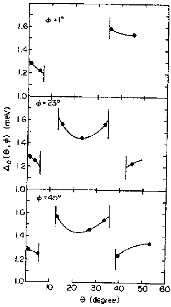
Figure 5: Gap anisotropy for Pb as a function of angle, $\theta$, for three different values of azimuthal angle, $\phi$. Regions where the Fermi surface of Pb does not exist are indicated by vertical lines. Figure reproduced from Ref. [122].

How big can the anisotropy be in pure conventional superconductors ? Microscopically the anisotropy is related to band structure anisotropy plus anisotropy in the electron-phonon spectral function from Eq. (16), $\alpha^{2}F({\bf k,k^{\prime}},\nu)$. In Fig. 5 we show the results of a calculation of the gap anisotropy in Pb as a function of position on the Fermi surface [122]. These calculations include multiple-plane-wave effects for the electronic wave functions, and the corresponding distortions of the Fermi surface from a sphere, as well as anisotropy effects due to the phonons and umklapp processes in the electron phonon interactions. The Figure illustrates the gap $\Delta_{\circ}(\theta,\phi)$ at zero temperature, as a function of $\theta$ for three constant $\phi$ arcs. Solid angle regions where the Fermi surface of Pb does not exist are indicated by vertical solid lines. It is clear that the pure Pb crystal gap is highly anisotropic, varying by about 20% over the Fermi surface. As described above, impurities will wash out this anisotropy. Nevertheless, such anisotropies can be observed in some low temperature properties, like the specific heat. For more details the reader is referred to Ref. [117].

The other complication we have mentioned is an energy variation in the EDOS, as seems to exist in some A15 compounds. If this energy dependence occurs on a scale comparable to $\omega_{D}$, then $N(\epsilon)$ cannot be assumed to be constant, and cannot be taken outside of the integrals in Eqs. (49-53). Such EDOS energy dependence is thought to be responsible for some of the anomalous properties seen in A15 compounds — their magnetic susceptibility and Knight shift [123], and the structural transformation from cubic to tetragonal [124, 125, 126]. Several electronic band structure calculations [127, 128, 129, 130] also find sharp structure in $N(\epsilon)$ at the Fermi level. An accurate description of the superconducting state thus requires a proper treatment of this structure. This was first undertaken to understand $T_{c}$ by Horsch and Reitschel [118] and independently by Nettel and Thomas [119]. A more general approach to understanding the effect of energy dependence in $N(\epsilon)$ on $T_{c}$ was given by Lie and Carbotte [120], who formulated the functional derivative $\delta T_{c}/\delta N(\epsilon)$; they found that only values of $N(\epsilon)$ within 5 to 10 times $T_{c}$ around the chemical potential have an appreciable effect on the value of $T_{c}$. More specifically they found that $\delta T_{c}/\delta N(\epsilon)$ is approximately a Lorentzian with center at the chemical potential; the function becomes negative only at energies $|\epsilon-\mu|{>\atop\sim}50T_{c}$.

Irradiation damage experiments illustrate some of this dependency. For example, irradiation of Mo₃Ge causes an increase in $T_{c}$ [131]. Washing out gap anisotropy with the irradiation cannot possibly account for an increase in $T_{c}$; instead, this result finds a natural explanation in the fact that the chemical potential for Mo₃Ge falls in a valley [132] of the EDOS, and irradiation smears the EDOS, thus increasing $N(\mu)$, and hence $T_{c}$.

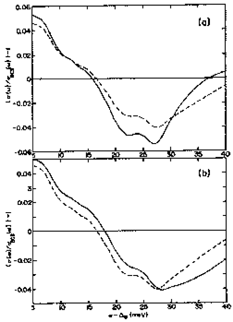
Figure 6: Normalized tunneling conductance reduced to the corresponding BCS expression, for (a) a peak, and (b) a valley in the electron density of states (solid curves). The dashed curves were obtained with a constant density of states. Reproduced from Ref. [134].

For details on the formulation of Eliashberg theory with an energy dependent $N(\epsilon)$ the reader is referred to the work of Pickett [133] and Mitrović and Carbotte [134], and references therein. The energy dependent EDOS affects many properties. To illustrate a typical result we show in Fig. 6 the effect of an energy dependent EDOS on the current (I)-voltage (V) characteristics of a tunneling junction [135, 134]. A detailed discussion of tunneling appears in Section 3.3.2. The tunneling conductance is proportional to the electron density of states, and is denoted by $\sigma(\omega)\equiv{\rm Re}\Biggl{(}{\omega\over\sqrt{\omega^{2}-\Delta^{2}(\omega)}}\Biggr{)}$. Fig. 6 shows the difference with the BCS conductance, $\sigma(\omega)/\sigma_{\rm BCS}(\omega)-1$ vs. $\omega-\Delta_{\circ}$ [134, 135]. Fig. 6a (b) is for a peak (valley) in the EDOS at the Fermi level. The solid curves include the effect of an energy dependent EDOS, while the dashed curves do not (the EDOS is approximated by a constant value, $N(\mu)$). In these examples the electron phonon spectral density obtained for Nb₃Sn [136] is used.

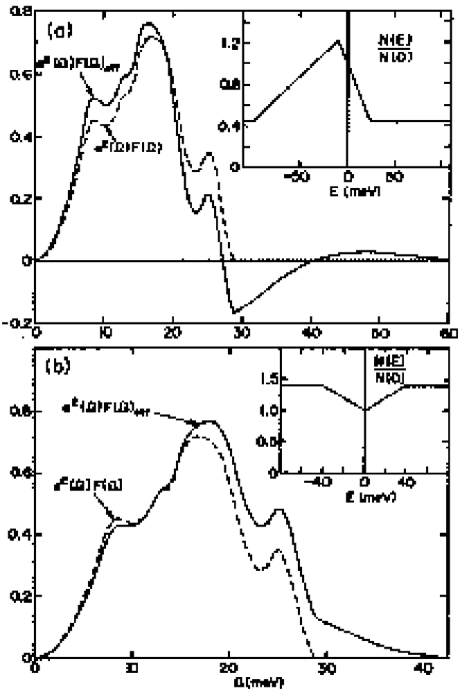
Figure 7: Effective electron phonon spectral functions obtained by the inversion of the calculated normalized tunneling conductances within the usual (i.e. constant electron density of states) Eliashberg theory (solid curves). The input spectral functions are shown with the dashed curves. The insets contain the corresponding electron densities of states used. Reproduced from Ref. [134].

These differences can be highlighted in another way, shown in Fig. 7 [135, 134]. Here, the “effective” electron phonon spectral density, $\alpha^{2}F(\Omega)_{\rm eff}$, is obtained by inverting the solid curves in Fig. 6 under the assumption that the EDOS is constant and equal to $N(\mu)$. The dashed curves give Shen’s original $\alpha^{2}F(\Omega)$ while the solid curves are the result of (incorrectly) inverting the result obtained with an energy dependent EDOS, but not accounting for it in the inversion process itself. The actual EDOS used to generate the I-V characteristic is shown in the inset for each figure. It contains a peak in Fig. 7a and a valley in Fig. 7b. Clearly a peak introduces a negative tail into $\alpha^{2}F(\Omega)_{\rm eff}$, which of course is not present in the actual $\alpha^{2}F(\Omega)$. For other important modifications the reader is referred to the references. The rest of this chapter will focus primarily on the ‘standard’ theory, using Eqs. (54-57) with $A_{0}(m)\equiv 1$ and $A_{1}(m)\equiv 0$.

All of the equations discussed so far have been developed on the imaginary frequency axis. Because practitioners in the field at the time were interested in tunneling spectroscopy measurements [49], the theory was first developed on the real frequency axis [4, 47]. The resulting equations are complicated, even for numerical solution. It wasn’t until quite a number of years later that numerical work returned to the imaginary axis [137], where, for thermodynamic properties, the numerical solution was very efficient [138, 139, 140, 141]. The difficulty, however, was that imaginary axis solutions are not suitable for dynamical properties. We will return to the interplay between imaginary and real frequency axis solutions as we ecounter them throughout the chapter.

3 The Phonons

3.1 Neutron Scattering

When dealing with model Hamiltonians, the phonon dispersion relations (before interaction with the electrons) are generally given, and simple: they are Einstein modes, or Debye-like modes, for example. A noteable exception is the case where the model contains anharmonic forces, in which case even the ‘non-interacting’ phonon spectrum is unknown.

In the case of real solids, and in particular metals, the situation is much worse. In this case the electrons cannot be ignored, though they can be treated in the Born-Oppenheimer approximation. Nonetheless the results require parametrization (with input from other experiments) and are generally not reliable. Pseudopotential methods [142, 143] can be applied to this problem, again, with limited success. In contrast, the spectacular success of inelastic neutron scattering techniques [89, 90] to simply measure the phonon dispersion curves in real metals effectively eliminates the need to calculate them quantitatively. Various qualitative effects, like the impact of electronic screening to the long wavelength ionic plasma mode [146], as well as the existence of Kohn anomalies [147], all due to the presence of electrons, are understood theoretically. For detailed results, however, Born-von Karman fits to high symmetry phonon dispersions suffice for an excellent description of the low temperature phonon properties. At temperatures of order $10$ K, the phonons in most conventional superconductors are completely determined, and no longer changing with temperature. Hence, as far as understanding (low temperature) superconductivity is concerned, these higher temperature measurements are sufficient.

The measured dispersion curves, $\omega_{\bf q}$ (again, branch indices are suppressed), are summarized in the frequency distribution

$$F(\nu)={1\over N}\sum_{\bf q}\delta(\nu-\omega_{\bf q}),$$ (62)

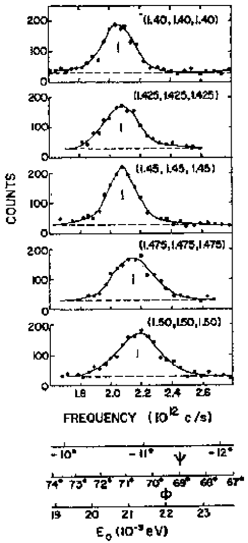
Figure 8: A set of ‘constant ${\bf q}$’ scans in Pb taken at various points along the diagonal in the Brillouin zone. Reproduced from Ref. [89].

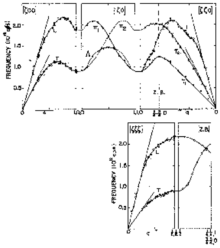
Figure 9: The dispersion curves for Pb at 100 K, as a function of momentum along various high symmetry directions. Reproduced from Ref. [89].

where $N$ is the number of ions in the system, and ${\bf q}$ is a wavevector which ranges over the entire First Brillouin Zone (FBZ), (and implicitly contains the branch index). It should be stressed that this procedure is an idealization; in actual fact a set of ‘constant ${\bf q}$’ scans are performed (usually along high symmetry directions). A typical result [89] is shown in Fig. 8 for Pb, for a set of wavevectors along the diagonal in reciprocal space. Note that the neutron counts tend to form a peak as a function of energy transfer (to the neutron), $\hbar\nu$. In general these peaks have a finite width, i.e. broader than the spectrometer resolution; these are due to a variety of effects, for example, anharmonic effects. Nonetheless, because the peaks are relatively sharp compared to the centroid energy, (i.e. the phonon inverse lifetimes are small compared to their energies), these data are usually presented in the form of Fig. 9, as a set of dispersion curves. Fig. 9 does obscure, however, the lifetimes of the various phonons, and hence the validity of Eq. (62), where infinitely long-lived phonons are assumed throughout the Brillouin zone, is called into question.

Nonetheless, for most of the Brillouin zone the approximation of infinitely long-lived excitations is a good one (hence, the name, phonon), and so the spectrum of excitations can be constructed according to Eq. (62). Such a procedure relies on coherent neutron scattering. An alternative is to use incoherent neutron scattering, whereby one measures the spectrum more or less directly. This latter procedure has advantages over the former, but also includes multiphonon scattering processes, and for non-elemental materials, weighs the contribution from each element differently, according to their varying scattering lengths. The result is often denoted the ‘generalized density of states’ (GDOS). A comparison for a Thallium-Lead alloy is shown in Fig. 10 [144, 145]. Also shown is the result from tunneling, to be discussed in the next subsection. There is clearly good agreement between the various methods. Amongst the two neutron scattering techniques, inelastic coherent neutron scattering produces the sharpest features, but requires a model (i.e. a Born-von Karman fit) to extract the spectrum $F(\nu)$ from the dispersion curves measured along high symmetry directions.

3.2 The Eliashberg Function, $\alpha^{2}F(\nu)$: Calculations

First-principle calculations of the electron-phonon spectral function, $\alpha^{2}F(\nu)$ require a knowledge of the electronic wave functions, the phonon spectrum, and the electron-phonon matrix elements between two single-electron Bloch states. A fairly comprehensive review is given in Ref. [88]. For our purposes, we note that, since the phonon spectrum will come from experiment, Eq. (16) requires calculation of $g_{\bf k,k^{\prime}}$. It is [11, 88]

$$g_{{\bf k,k^{\prime}}j}=<\psi_{\bf k}\mid{\bf\epsilon}^{j}({\bf k-k^{\prime}})\cdot{\bf\nabla V}\mid\psi_{\bf k^{\prime}}>\left[{\hbar\over 2M\omega_{j}({\bf k-k^{\prime}})}\right]^{1/2}$$ (63)

where, for this equation we have included the phonon branch index $j$ explicitly. The Bloch state is denoted $\mid\psi_{\bf k}>$, and ${\bf\epsilon}^{j}({\bf k})$ is the polarization vector for the ($j{\bf k}$)th phonon mode. The crystal potential is denoted $V$, and as one might expect, the electron-phonon coupling depends on its gradient.

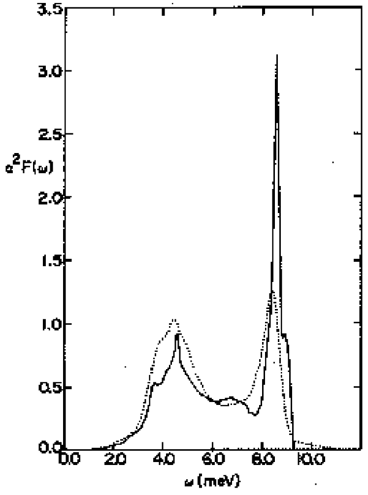
Figure 11: The electron phonon spectral function $\alpha^{2}F(\omega)$ measured in tunneling experiments (dotted curve) compared with that which is calculated from first principles (solid curve) [148].

Tomlinson and Carbotte [148] used pseudopotential methods [149, 150] to compute $g_{{\bf k,k^{\prime}}j}$ and, from Eq. (16), $\alpha^{2}F(\nu)$, for Pb. The phonons were taken from experiment [89, 90, 151, 152] through Born - von Kármán fits. The result is plotted in Fig. 11, along with results from tunneling experiments (to be described below). The agreement is qualitatively very good; this provides very strong confirmation of the electron phonon mechanism of superconductivity.

Further details of more modern calculations of electron-phonon coupling constants can be found in, for example, Refs. [76] and [77] and references therein. Their reliability appears to remain an issue, both with the high temperature cuprates, and perhaps less so with the fulleride and more conventional superconductors. The spirit of these calculations is somewhat different than the older ones, in that coupling constants are extracted from the phonon linewidths, where it is assumed that the phonon broadening is entirely due to the electron-ion interaction (and not, say, anharmonic effects). Allen [153, 154] derived a formula (Fermi’s Golden Rule) for the inverse lifetime, $\gamma_{\bf q}(\nu)$, of a phonon with momentum (and branch index) ${\bf q}$:

$$\gamma_{\bf q}=2\pi\omega_{\bf q}\sum_{\bf k}|g_{{\bf k,k^{\prime}}}|^{2}\left[{f({\epsilon_{\bf k+q}}-\mu)-f({\epsilon_{\bf k}}-\mu)\over\hbar\omega_{\bf q}}\right]\delta(\epsilon_{\bf k+q}+\hbar\omega_{\bf q}-\epsilon_{\bf k}),$$ (64)

where again we have suppressed both phonon branch indices and electron band labels. Using this equation, in the approximation that the expression $\left[f(\epsilon_{\bf k+q}-\mu)-f(\epsilon_{\bf k}-\mu)\right]/(\hbar\omega_{\bf q})$ is replaced by $\delta({\epsilon_{\bf k}}-\mu)$ makes it resemble Eq. (17), so that one can write

$$\alpha^{2}F(\nu) = {1\over\pi N(\mu)}{1\over N}\sum_{\bf q}{1\over 2}{\gamma_{\bf q}\over\hbar\omega_{\bf q}}\delta(\nu-\omega_{\bf q})$$ (65)

$$= {1\over 3N}\sum_{\bf q}{1\over 2}\omega_{\bf q}\lambda_{\bf q}\delta(\nu-\omega_{\bf q})$$

where the second line serves to define a ${\bf q}$-dependent coupling parameter:

$$\lambda_{\bf q}\equiv{3\over\pi N(\mu)}{\gamma_{\bf q}\over\hbar\omega^{2}_{\bf q}}.$$ (66)

It is through these relations that coupling parameters are often determined.

It is worth noting at this point that several moments of the function $\alpha^{2}F(\nu)$ have played an important role in characterizing retardation (and strong coupling) effects in superconductivity. Foremost amongst these is the mass enhancement parameter, $\lambda$, already defined in Eq. (20); in addition, the characteristic phonon frequency, $\omega_{\ln}$ is given by

$$\omega_{\ln}\equiv\exp{\left[{2\over\lambda}\int_{0}^{\infty}d\nu\,\ln{(\nu)}{\alpha^{2}F(\nu)\over\nu}\right]}.$$ (67)

Further discussion of these calculations can be found in Refs. [88, 11].

3.3 Extraction from Experiment

Experiments which probe dynamical properties do so as a function of frequency, which is a real quantity. However, the Eliashberg equations as formulated in the previous section are written on the imaginary frequency axis. To extract information from these equations relevant to spectroscopic experiments, one must analytically continue these equations to the real frequency axis. Mathematically speaking, this is not a unique procedure; one can often imagine several functions whose values on the imaginary axis are equal, and yet differ elsewhere in the complex plane (and in particular on the real axis). For example, replacing unity by $-\exp{(\beta i\omega_{m})}$, in any number of places in the equations does not affect the imaginary axis equations, or their solutions, and yet on the real axis the corresponding number of factors $-\exp{(\beta\omega)}$ will appear.

Physically speaking, however, the Green functions involved have to satisfy certain conditions; complying with these conditions determines the function uniquely [93]. This allows a unique determination of the analytic continuation of the Eliashberg equations on the real axis. This procedure will be discussed in the following subsection, followed by subsections on experimental spectroscopies, and how they can be used to extract the Eliashberg function, $\alpha^{2}F(\nu)$.

3.3.1 The Real-Axis Eliashberg Equations

We begin with Eqs. (42 - 46). To analytically continue Eqs. (44 - 46) is trivial; one simply replaces the imaginary frequency $i\omega_{m}$ wherever it appears with $\omega+i\delta$. The $i\delta$ remains to remind us that we are analytically continuing the function to just above the real axis; it is important to specify this since there is a discontinuity in the Green function as one crosses the real axis. A simple replacement of $i\omega_{m}$ with $\omega+i\delta$ in Eqs. (42,43) (leaving the summations over $m^{\prime}$) would in general be incorrect. The correct procedure is to first perform the Matsubara sum, and then make the replacement. To perform the Matsubara sum, however, one has to introduce the spectral representation for the Green functions, $G$ and $F$. These are given by

$$G({\bf k},i\omega_{m}) = \int_{-\infty}^{\infty}d\omega\,{A({\bf k},\omega)\over i\omega_{m}-\omega}$$ (68)

$$F({\bf k},i\omega_{m}) = \int_{-\infty}^{\infty}d\omega\,{C({\bf k},\omega)\over i\omega_{m}-\omega},$$ (69)

where $A({\bf k},\omega)$ is given by Eq. (26) and $C({\bf k},\omega)$ is given by a similar relation:

$$C({\bf k},\omega)\equiv-{1\over\pi}{\rm Im}F({\bf k},\omega+i\delta).$$ (70)

The spectral representation for the phonons is already present in Eqs. (42,43). Therefore the Matsubara sum can be performed straightforwardly (see, for example, Refs. [83, 13]), and the analytical continuation can be done. Upon integrating over momentum (using, as in Eqs. (54-57) electron-hole symmetry and a constant (and infinite in extent) density of electron states), one arrives at the standard real-axis Eliashberg equations [4, 13]. These equations are much more difficult to solve than the imaginary axis counterparts. They require numerical integration of principal value integrals and square-root singularities, and the various Green function components are complex. In contrast the imaginary axis equations are amenable to computers (the sums are discrete) and the quantities involved are real. Moreover a considerable number of thermodynamic and magnetic properties can be obtained directly from the imaginary axis solutions.

The discrepancy in computational ease between the two formulations led to an alternative path to dynamical information, namely the direct analytic continuation of the solutions of the imaginary axis equations to the real axis by a fitting procedure with Padé approximants [155]. This method is in general very sensitive to the input data, and has (surmountable [156, 157]) difficulties at high temperatures and frequencies.

More recently yet another procedure was formulated [158], which first requires a numerical solution of the imaginary axis equations, followed by a numerical solution of analytic continuation equations. This latter set is formally exact (i.e. no fitting required) and yet avoids the complications of the real-axis equations. These equations are

$$\Sigma({\bf k},z)={1\over N\beta}\sum_{{\bf k^{\prime}}m^{\prime}=-\infty}^{\infty}{\lambda_{{\bf k}{\bf k^{\prime}}}(z-i\omega_{m^{\prime}})\over N(\mu)}G({\bf k^{\prime}},i\omega_{m^{\prime}})\phantom{a}-\phantom{{1\over N\beta}\sum_{{\bf k^{\prime}}m^{\prime}=-\infty}^{\infty}{\lambda_{{\bf k}{\bf k^{\prime}}}(z-i\omega_{m^{\prime}})\over N(\mu)}G({\bf k^{\prime}},i\omega_{m^{\prime}})}$$

$${1\over N}\sum_{{\bf k^{\prime}}}\int_{0}^{\infty}d\nu{\alpha_{{\bf k}{\bf k^{\prime}}}^{2}F(\nu)\over N(\mu)}\Biggl{\{}\Bigl{[}f(\nu-z)+N(\nu)\Bigr{]}G({\bf k^{\prime}},z-\nu)+\Bigl{[}f(\nu+z)+N(\nu)\Bigr{]}G({\bf k^{\prime}},z+\nu)\Biggr{\}}$$ (71)

$$\phi({\bf k},z)={1\over N\beta}\sum_{{\bf k^{\prime}}m^{\prime}=-\infty}^{\infty}\Biggl{[}{\lambda_{{\bf k}{\bf k^{\prime}}}(z-i\omega_{m^{\prime}})\over N(\mu)}-V_{{\bf k}{\bf k^{\prime}}}\Biggr{]}F({\bf k^{\prime}},i\omega_{m^{\prime}})\phantom{a}-\phantom{\Biggl{[}{\lambda_{{\bf k}{\bf k^{\prime}}}(z-i\omega_{m^{\prime}})\over N(\mu)}-U\Biggr{]}F({\bf k^{\prime}},i\omega_{m^{\prime}})}$$

$${1\over N}\sum_{{\bf k^{\prime}}}\int_{0}^{\infty}d\nu{\alpha_{{\bf k}{\bf k^{\prime}}}^{2}F(\nu)\over N(\mu)}\Biggl{\{}\Bigl{[}f(\nu-z)+N(\nu)\Bigr{]}F({\bf k^{\prime}},z-\nu)+\Bigl{[}f(\nu+z)+N(\nu)\Bigr{]}F({\bf k^{\prime}},z+\nu)\Biggr{\}},$$ (72)

where $z$ can actually be anywhere in the upper half-plane. Thus, for example, Eqs. (42,43) can be recovered by substituting $z=i\omega_{m}$. On the other hand, once these equations have been solved, one can substitute $z=\omega+i\delta$, and iterate the resulting equations to convergence. When the “standard” approximations for the momentum dependence are made (i.e. Fermi surface averaging, constant density of states, particle-hole symmetry, etc.) the result is

$$Z(\omega+i\delta) = 1+{i\pi T\over\omega}\sum_{m=-\infty}^{\infty}\lambda(\omega-i\omega_{m}){\omega_{m}Z(i\omega_{m})\over\sqrt{\omega_{m}^{2}Z^{2}(i\omega_{m})+\phi^{2}(i\omega_{m})}}$$ (73)

$$+{i\pi\over\omega}\int_{0}^{\infty}d\nu\,\alpha^{2}F(\nu)\Biggl{\{}\bigl{[}N(\nu)+f(\nu-\omega)\bigr{]}{(\omega-\nu)Z(\omega-\nu+i\delta)\over\sqrt{(\omega-\nu)^{2}Z^{2}(\omega-\nu+i\delta)-\phi^{2}(\omega-\nu+i\delta)}}$$

$$+\bigl{[}N(\nu)+f(\nu+\omega)\bigr{]}{(\omega+\nu)Z(\omega+\nu+i\delta)\over\sqrt{(\omega+\nu)^{2}Z^{2}(\omega+\nu+i\delta)-\phi^{2}(\omega+\nu+i\delta)}}\Biggr{\}}$$

$$\phi(\omega+i\delta) = \pi T\sum_{m=-\infty}^{\infty}\bigl{[}\lambda(\omega-i\omega_{m})-\mu^{*}(\omega_{c})\theta(\omega_{c}-|\omega_{m}|)\bigr{]}{\phi(i\omega_{m})\over\sqrt{\omega_{m}^{2}Z^{2}(i\omega_{m})+\phi^{2}(i\omega_{m})}}$$ (74)

$$+i\pi\int_{0}^{\infty}d\nu\,\alpha^{2}F(\nu)\Biggl{\{}\bigl{[}N(\nu)+f(\nu-\omega)\bigr{]}{\phi(\omega-\nu+i\delta)\over\sqrt{(\omega-\nu)^{2}Z^{2}(\omega-\nu+i\delta)-\phi^{2}(\omega-\nu+i\delta)}}$$

$$+\bigl{[}N(\nu)+f(\nu+\omega)\bigr{]}{\phi(\omega+\nu+i\delta)\over\sqrt{(\omega+\nu)^{2}Z^{2}(\omega+\nu+i\delta)-\phi^{2}(\omega+\nu+i\delta)}}\Biggr{\}}.$$

Note that in cases where the square-root is complex, the branch with positive imaginary part is to be chosen.

One important point has been glossed over in these derivations. Because of the infinite bandwidth approximation, an unphysical divergence occurs in the term involving the direct Coulomb repulsion, $V_{\bf k,k^{\prime}}$, both in the imaginary axis formulation, Eq. (56), and in the real-axis formulation, Eq. (74). The solution to this difficulty is to introduce a cutoff in frequency space (even though the original premise was that the Coulomb repulsion was frequency independent), as is apparent in the two equations. In fact, this cutoff should be of order the Fermi energy, or bandwidth. However, this requires a summation (or integration) out to huge frequency scales. In fact one can use a scaling argument [159, 3, 160] to replace this summation (or integration) by one which spans a small multiple ($\approx 6$) of the phonon frequency range. Hence the magnitude of the Coulomb repulsion is scaled down, and becomes [159]

$$\mu^{\ast}(\omega_{c})\approx{N(\mu)U\over 1+N(\mu)U\ln{\epsilon_{F}\over\omega_{c}}},$$ (75)

where $U$ is a double Fermi surface average of the direct Coulomb repulsion. This reduction is correct physically, in that the retardation due to the phonons should reduce the effectiveness of the direct Coulomb repulsion towards breaking up a Cooper pair. It does appear to overestimate this reduction, however [161]. The analytic continuation of this part of the equations has been treated in detail in Ref. [162].

In the zero temperature limit, Eqs. (73,74) are particularly simple. Then the Bose function is identically zero and the Fermi function becomes a step function: $f(\nu-\omega)\rightarrow\theta(\omega-\nu)$. Once the imaginary axis equations have been solved, solution of Eqs. (73,74) no longer requires iteration. One can simply build up the solution by construction from $\omega=0$ (assuming $\alpha^{2}F(\nu)$ has no weight at $\nu=0$); in fact, if the phonon spectrum has no weight below a frequency, $\nu_{\rm min}$, then only the first lines in Eqs. (73,74) need be evaluated. In particular, if the gap (still to be defined) happens to occur below this minimum frequency (often a good approximation for a conventional superconductor) then the gap can be obtained in this manner [163].

In the following two sections we explore the possibility of using Eqs. (73,74) to obtain information about the microscopic parameters of Eliashberg theory.

3.3.2 Tunneling

Perhaps the simplest, most direct probe of the excitations of a solid is through single particle tunneling. In this experiment electrons are injected into (or extracted from) a sample, as a function of bias voltage, $V$. The resulting current is proportional to the superconducting density of states [48, 164, 165, 166]:

$$I_{S}(V)\propto\int d\omega{\rm Re}\left[{|\omega|\over\sqrt{\omega^{2}-\Delta^{2}(\omega)}}\right]\left[f(\omega)-f(\omega+V)\right],$$ (76)

where we have used the gap function, $\Delta(\omega)$, defined as

$$\Delta(\omega)\equiv\phi(\omega+i\delta)/Z(\omega+i\delta).$$ (77)

The proportionality constant contains information about the density of states in the electron supplier (or acceptor), and the tunneling matrix element. These are usually assumed to be constant. If one takes the zero temperature limit, then the derivative of the current with respect to the voltage is simply proportional to the superconducting density of states,

$$\left({dI\over dV}\right)_{S}/\left({dI\over dV}\right)_{N}={\rm Re}\left(|V|\over\sqrt{V^{2}-\Delta^{2}(V)}\right),$$ (78)

where $S$ and $N$ denote “superconducting” and “normal” state, respectively. The right hand side of Eq. (78) is simply the density of states, computed within the Eliashberg framework (see, for example, Ref. [52]). It is not at all apparent what the structure of the density of states is from Eq. (78), until one has solved for the gap function from Eqs. (73,74) and Eq. (77). At zero temperature the gap function $\Delta(\omega)$ is real and roughly constant up to a frequency roughly equal to that constant. This implies that the density of states will have a gap, as in BCS theory. At finite temperature the gap function has a small imaginary part starting from zero frequency (and, in fact the real part approaches zero at zero frequency [167]) so that in principle there is no gap, even for an s-wave order parameter. In practice, a very well-defined gap still occurs for moderate coupling, and disappears at finite temperature only when the coupling strength is increased significantly [168, 169].

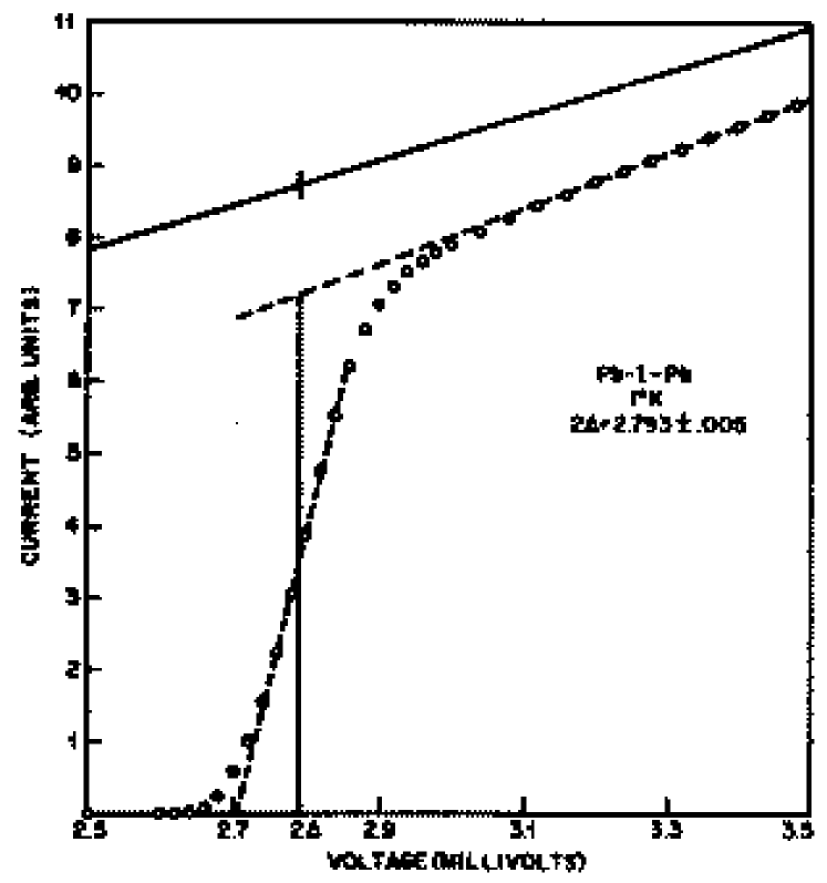
Figure 12: I-V characteristic of a Pb-I-Pb junction showing the construction used to find the energy gap. The solid line and open circles are the current in the normal and superconducting states, respectively. Reproduced from Ref. [52].

In Fig. 12 and 13 we show the current-voltage and conductance plots for superconducting Pb, taken from McMillan and Rowell [52]. These data were obtained from a superconductor-insulator-superconductor (SIS) junction, with Pb being the superconductor on both sides of the insulating barrier, so that, rather than directly using Eq. (78), the current is given by a convolution of the two superconducting densities of states. Two features immediately stand out in these plots. First, a gap is clearly present in Fig. 12, given by $2\Delta_{\circ}$, where $\Delta_{\circ}$ is the single electron gap defined by

$$\Delta_{\circ}\equiv{\rm Re}\Delta(\omega=\Delta_{\circ}),$$ (79)

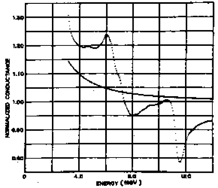
Figure 13: Conductance $dI/dV$ of a Pb-I-Pb junction in the superconducting state normalized by the conductance in the normal state vs. voltage. Also shown is the two-superconductor conductance calculated from the BCS density of states which contains no phonon structure. Reproduced from Ref. [52].

a definition one can use for all temperatures. Secondly, a significant amount of structure occurs beyond the gap region, as is illustrated in Fig. 13.

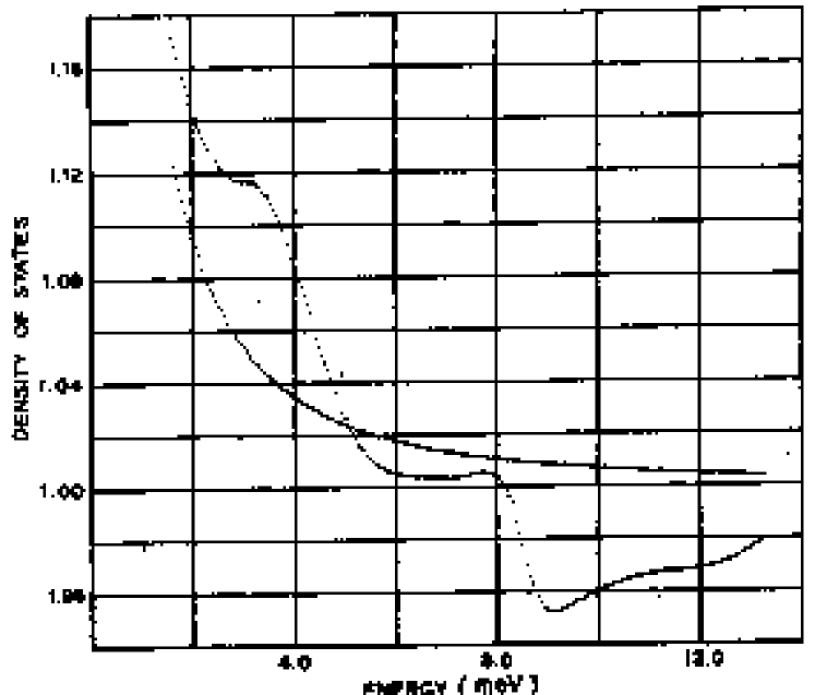
Figure 14: Electronic density of states $N(E)$ vs. $E-\Delta_{\circ}$ for Pb, obtained from the data of Fig. 13. The smooth curve is the BCS density of states. Reproduced from Ref. [52].

McMillan and Rowell were able to deconvolve their measurement, to produce the single electron density of states shown in Fig. 14. Since the superconducting density of states is given by the right hand side of Eq. (78), the structure in the data must be a reflection of the structure present in the gap function, $\Delta(\omega)$. The structure in the gap function is in turn a reflection of the structure in the input function, $\alpha^{2}F(\nu)$. In other words, Eqs. (73,74) can be viewed as as a highly nonlinear transform of $\alpha^{2}F(\nu)$. Thus the structure present in Fig. 14 contains important information (in coded form) concerning the electron-phonon interaction. One has only to “invert” the “transform” to determine $\alpha^{2}F(\nu)$ from the tunneling data. This is precisely what McMillan and Rowell [50, 52] accomplished, first in the case of Pb.

The procedure to do this is as follows. First a “guess” is made for the entire function, $\alpha^{2}F(\nu)$, and the Coulomb pseudopotential parameter, $\mu^{\ast}$. Then the real axis Eliashberg equations ((72) and (73)) are solved, and the superconducting density of states (Eq. (78)) is calculated. The result attained will in general differ from the experimentally measured function (represented, for example, by Fig. 14); a Newton-Raphson procedure (using functional derivatives rather than normal derivatives) is used to determine the correction to the initial guess for $\alpha^{2}F(\nu)$ that will lead to better agreement. Very often another parameter (for example, the measured energy gap value) is used to fit $\mu^{\ast}$. This process is iterated until convergence is achieved. The result for Pb is illustrated by the dotted curve in Fig. 11.

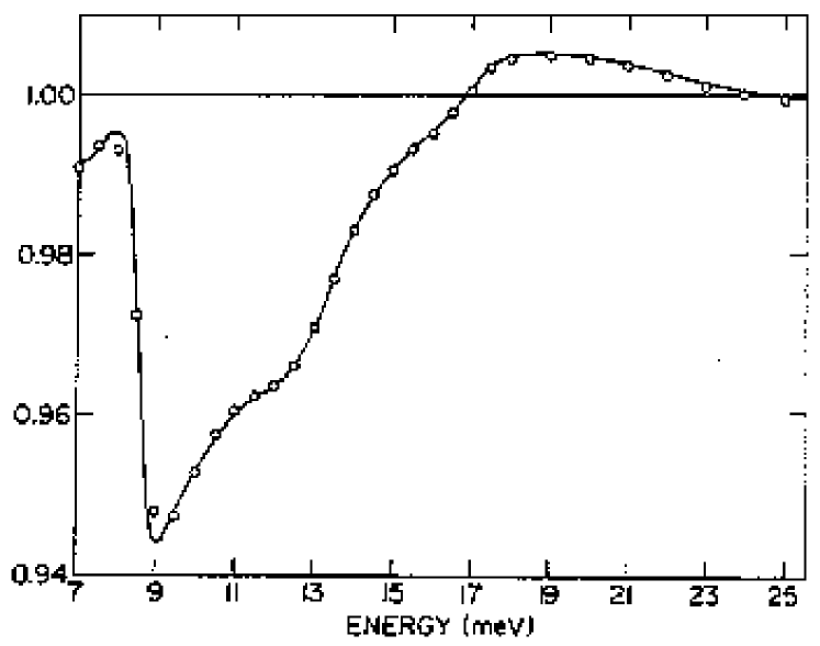
Figure 15: The predicted (solid curve) normalized density of states in Pb as a function of energy $\omega$ compared with measured values (open dots) as a function of energy measured from the gap edge. The measured density of states divided by the BCS density of states above 11 meV was not used in the fitting procedure that produced $\alpha^{2}F(\omega)$ and a comparison of theory and experiment in the multiple-phonon region is a valid test of the theory. Reproduced from Ref. [52].

Once $\alpha^{2}F(\nu)$ (and $\mu^{\ast}$) has been acquired in this way one can use the Eliashberg equations to calculate other properties, for example, $T_{c}$. These can then be compared to experiment, and the agreement in general tends to be fairly good. One may suspect, however, a circular argument, since the theory was used to produce the spectrum (from experiment), and now the theory is used as a predictive tool, with the same spectrum. There are a number of reasons, however, for believing that this procedure has produced meaningful information. First, the spectrum attained has come out to be positive definite, as is required physically. Second, the spectrum is non-zero precisely in the phonon region, as it should be. Moreover, it agrees very well with the calculated spectrum. Thirdly, as already mentioned, various thermodynamic properties are calculated with this spectrum, with good agreement with experiment. Finally, the density of states itself can be calculated in a frequency regime beyond the phonon region, as is shown in Fig. 15. The agreement with experiment is spectacular.

None of these indicators of success can be taken as definitive proof of the electron-phonon interaction. For example, even the excellent agreement with the density of states could be understood as a mathematical property of analytic functions [170]. Also, we have focussed on Pb; in other superconductors this procedure has not been so straightforward. For example, in Nb a proximity layer is explicitly accounted for in the inversion [171, 166], thus introducing extra parameters. In the so-called A15 compounds (eg. Nb₃Sn, V₃Si, etc.), although the measured tunneling results have been inverted [172], several experiments do not fit the overall electron-phonon framework [10].

More details are provided in Ref. [11]. An alternate inversion procedure is also provided there [173], which utilizes a Kramers-Kronig relation to extract $\Delta(\omega)$ from the tunneling result. An inversion of ${\rm Im}\phi(\omega+i\delta)$ then removes $\mu^{\ast}$ from the procedure. A variant of this, where the imaginary axis quantity $\Delta(i\omega_{m})$ is extracted directly from the tunneling I-V characteristic, and then the imaginary axis equations are inverted for $\alpha^{2}F(\nu)$, also works [174], but the accuracy requirements for a unique inversion are very debilitating.

3.3.3 Optical Conductivity

In principle, any spectroscopic measurement will contain a signature of $\alpha^{2}F(\nu)$. In particular, several attempts have been made to infer $\alpha^{2}F(\nu)$ from optical conductivity measurements in the superconducting state [175, 176, 177]. In this section we describe a procedure for extracting $\alpha^{2}F(\nu)$ from the normal state [178].

A common method to determine the optical conductivity is to measure the reflectance [179] as a function of frequency, usually at normal incidence. The reflectance, $R(\nu)$, is defined as the absolute ratio squared of reflected over incident electromagnetic wave amplitude. The complex reflectivity is defined by

$$r(\nu)\equiv R^{1/2}(\nu)\exp{(i\theta(\nu))},$$ (80)

where $\theta(\nu)$ is the phase, and is obtained through a Kramers-Kronig relation from the reflectance [179]

$$\theta(\nu)={\nu\over\pi}\int_{0}^{\infty}{\ln{R(\nu^{\prime})}-\ln{R(\nu)}\over\nu^{2}-{\nu^{\prime}}^{2}}d\nu^{\prime}.$$ (81)

The complex reflectivity is related to the complex index of refraction, $n(\nu)$,

$$r(\nu)\equiv{1-n(\nu)\over 1+n(\nu)},$$ (82)

which, finally, is related to the complex conductivity, $\sigma(\nu)$ (using the dielectric function, $\epsilon(\nu)$):

$$\epsilon(\nu)\equiv n^{2}(\nu)=\epsilon_{\infty}+{4\pi i\sigma(\nu)\over\nu},$$ (83)

where $\epsilon_{\infty}$ is the dielectric function at high frequency (in principle, for infinite frequency this would be unity). It is through such transformations that the ‘data’ is often presented in ‘raw’ form. Nonetheless, assumptions are required to proceed through these steps; for example, Eq. (81) indicates quite clearly that the reflectance is required over all positive frequencies. Thus extrapolation procedures are required at low and high frequencies; a more thorough discussion can be found in [180]; see also [181].

For this review, we will consider both static impurities and phonons as sources of electron scattering. Both contribute to the optical conductivity, and can be treated theoretically either with the Kubo formalism or with a Boltzmann approach [83]. In the Born approximation the result for the conductivity, in the normal state, at zero temperature, is [176]:

$$\sigma(\nu)={\omega^{2}_{P}\over 4\pi}{i\over\nu}\int_{0}^{\nu}d\omega{1\over\nu+i/\tau-\Sigma(\omega)-\Sigma(\nu-\omega)}$$ (84)

where

$$\Sigma(\omega)=\int_{0}^{\infty}d\Omega\alpha^{2}F(\Omega)\ln|{\Omega-\omega\over\Omega+\omega}|-i\pi\int_{0}^{|\omega|}d\Omega\ \alpha^{2}F(\Omega)$$ (85)

is the effective electron self-energy due to the electron-phonon interaction. The spectral function that appears in Eq. (85) is really a closely related function, as has been discussed by Allen [176] and Scher [182]. For our purposes we will treat them identically. The other two parameters that enter these expressions are the electron plasma frequency, $\omega_{P}$, and the (elastic) electron-impurity scattering rate, $1/\tau$.

Equation (84) has been written to closely resemble the Drude form,

$$\sigma_{\rm Dr}(\nu)={\omega_{P}^{2}\over 4\pi}{i\over\nu+i/\tau};$$ (86)

the equation could well be recast in this form, with a frequency-dependent scattering rate and effective mass (in the plasma frequency) [183]. Eqs. (84) and (85) make clear that the optical conductivity is given by two integrations over the electron-phonon spectral function. One would like to “unravel” this information as much as possible before attempting an inversion, so that, in effect, the signal is “enhanced”. To this end one can attempt various manipulations [184, 185, 186].

As a first step one can make a weak coupling type of approximation to obtain [178] the explicit result:

$$\alpha^{2}F(\nu)={1\over 2\pi}{\omega_{P}^{2}\over 4\pi}{d^{2}\over d\nu^{2}}\biggl{\{}\nu Re{1\over\sigma(\nu)}\biggr{\}}.$$ (87)

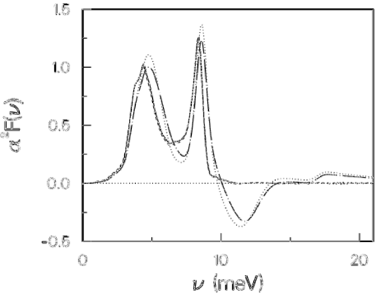
Figure 16: $\alpha^{2}F(\nu)$ for Pb (solid curve) vs. $\nu$, along with the estimates obtained from Eq. (87) with an impurity scattering rate, $1/\tau=1$ meV (dotted) and 10 meV (dot-dashed). These are both qualitatively quite accurate, before they become negative at higher frequencies. Also plotted is the result (dashed curve, indiscernible from the solid curve) obtained from a full numerical inversion, as described in the text. Taken from the second reference in Ref. [178].

Note that the conductivity data, including a measurement of the plasma frequency, provides us with both the shape and magnitude of $\alpha^{2}F(\nu)$. Eq. (87) works extremely well, as Fig. 16 shows, in the case of Pb. It tells us that, with a judicious manipulation of the conductivity data, the underlying electron-phonon spectral function emerges in closed form. The very simple formula, Eq. (87) introduces some errors — it was derived with some approximations — as can be seen in Fig. 16. In fact, a full numerical inversion will also succeed [187, 188]; the first reference requires a Newton-Raphson iteration technique, while the second uses an adaptive method (in the superconducting state).

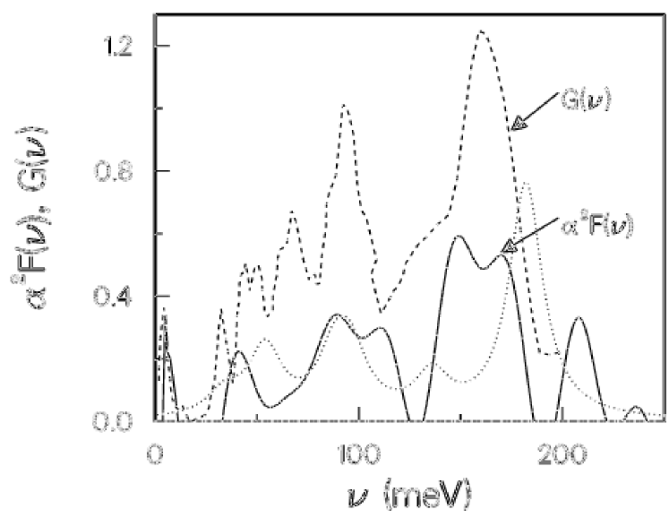
Figure 17: The $\alpha^{2}F(\nu)$ for K₃C₆₀ (solid curve) extracted from the reflectance data of Degiorgi et al. [314], using Eq. (87). For purposes of analysis we have omitted the negative parts. The neutron scattering results from Ref. [189] (dashed curve) are also shown. Clearly the energy scale in $\alpha^{2}F(\nu)$ matches that of the phonons, and some of the peaks even line up correctly. Finally, the dotted curve comes from an analysis of photoemission data [190], where we have arbitrarily broadened the phonon spectrum with Lorentzian lineshapes. Taken from the second reference in Ref. [178].

Eq. (87) was first applied to K₃C₆₀ [178] to help determine whether or not this class of superconductor was driven by the electron-phonon interaction. The result is shown in Fig. 17 and provides convincing evidence that the alkali-doped fullerene superconductors are driven by the electron-phonon mechanism. We will return to these superconductors in a later section, and further examine the optical conductivity in the superconducting state in another section.

4 The Critical Temperature and the Energy Gap

Perhaps the most important property of a superconductor is the critical temperature, $T_{c}$. For this reason a considerable amount of effort has been devoted both towards new materials with higher superconducting $T_{c}$, and, on the theoretical side, towards an analytical solution of the linearized Eliashberg equations (set $\phi{{}_{m}{{}^{\prime}}}$ to zero, where it appears in the denominator in Eqs. (54 - 57) ) for $T_{c}$ (see [13, 11] for reviews); the experimental ‘holy grail’ has enjoyed some success, particularly in the last 15 years; the theoretical goal has had limited success. In fact numerical solutions are so readily available at present, that the absence of an analytical solution is not really debilitating to understanding $T_{c}$.

In the conventional theory there are two input ”parameters”: a function of frequency, $\alpha^{2}F(\nu)$, about which we have already said much, and $\mu^{\ast}(\omega_{c})$, a number which summarizes the (reduced) Coulomb repulsion experienced by a Cooper electron pair. The focus of this chapter will be the effect of size and functional form of $\alpha^{2}F(\nu)$ on $T_{c}$.

4.1 Approximate Solution: The BCS Limit

The first insight into $T_{c}$ comes from reducing the Eliashberg theory to a BCS-like theory. This is accomplished by approximating the kernel

$$\lambda(i\omega_{m}-i\omega_{m^{\prime}})\equiv\int_{0}^{\infty}{2\nu\alpha^{2}F(\nu)\over\nu^{2}+(\omega_{m}-\omega_{m^{\prime}})^{2}}$$ (88)

by a constant as long as the magnitude of the two Matsubara frequencies are within a frequency rim of the Fermi surface [140], taken for convenience to be $\omega_{c}$, the cutoff used for the Coulomb repulsion, $\mu^{\ast}$. That is,

$$\lambda(i\omega_{m}-i\omega_{m^{\prime}})=\cases{\lambda\phantom{aaaa}{\rm for\phantom{aa}both}\phantom{aaaa}|\omega_{m}|,|\omega_{m^{\prime}}|<\omega_{c},\cr 0\phantom{aaaa}{\rm otherwise,}}$$ (89)

where $\lambda\equiv\lambda(0)$ has already been defined in Eq. (20). Then, the linearized version of Eq. (54) (with $A_{0}(m^{\prime})=1$), for the renormalization function, $Z(i\omega_{m})$, reduces to

$$Z(i\omega_{m})\approx 1+\lambda.$$ (90)

Using this and solving the linearized version of Eq. (56) for the pairing function yields

$${1+\lambda\over\lambda-\mu^{\ast}}=\psi\biggl{(}{\omega_{c}\over 2\pi T_{c}}+{1\over 2}\biggr{)}-\psi\bigl{(}{1\over 2}\bigr{)},$$ (91)

where $\psi(x)$ is the digamma function. The cutoff in these equations is along the Matsubara frequency axis; this procedure is to be contrasted with the BCS procedure, which introduced a cutoff in momentum space. The former is more physical, insofar as the true electron-phonon interaction comes from retardation effects, which occur in the temporal domain; hence the cutoff should occur in the frequency (either real, or imaginary) domain. In practice, the two procedures are connected, so they produce the same physical equation in the weak coupling limit.

Returning to Eq. (91), for large $x$, $\psi(x)\approx\log{(x)}$, so, in the weak coupling limit ($T_{c}<<\omega_{c}$), we obtain a BCS-like equation,

$$T_{c}=1.13\omega_{c}\exp{\biggl{(}-{1+\lambda\over\lambda-\mu^{\ast}}\biggr{)}}.$$ (92)

This equation has essentially summarized all the detailed information contained in the electron-phonon spectral function $\alpha^{2}F(\nu)$ into two parameters, $\lambda$ and $\omega_{c}$. The mass enhancement parameter, $\lambda$, is a simple moment of $\alpha^{2}F(\nu)$ (see Eq. (20)), while the parameter $\omega_{c}$ physically is meant to represent some typical phonon frequency. In more refined treatments [191, 140], $\omega_{c}$ is given by some moment of $\alpha^{2}F(\nu)$ as well. For example, in Ref. [140], the logarithmic average is used to define $\omega_{\ln}$ (see Eq. (67)), a quantity we shall use extensively in the following sections. They modified the McMillan equation [191] to read

$$k_{B}T_{c}={\hbar\omega_{\ln}\over 1.2}\exp{\biggl{(}-{1.04(1+\lambda)\over\lambda-\mu^{\ast}(1+0.62\lambda)}\biggr{)}}.$$ (93)

A derivation of this equation is given in Refs. [191, 140].

4.2 Maximum $T_{c}$, Asymptotic Limits, and Optimal Phonon Spectra

Eq. (92) (or Eq. (93)) describes the weak coupling limit of Eliashberg theory reasonably well. It errs in the strong coupling limit; for example, it predicts that $T_{c}$ saturates as $\lambda$ increases, whereas the Eliashberg equations themselves predict that $T_{c}$ grows indefinitely with $\lambda$ [192]. Asymptotic results from Eliashberg theory can be obtained correctly and analytically [140, 193, 11] through a variety of arguments. The methodology based on scaling theorems is particularly powerful, and has been applied to other thermodynamic properties as well [11].

The correct asymptotic result for $T_{c}$ is [140, 193]:

$$T_{c}=0.183\sqrt{\lambda}\omega_{E},$$ (94)

as $\lambda\rightarrow\infty$. In obtaining Eq. (94), an Einstein spectrum has been assumed (this is not required), which in turn is characterized by two parameters: the weight, $A\equiv\lambda\omega_{E}/2$, and the frequency, $\omega_{E}$. In writing Eq. (94), one tacitly has assumed that the parameter $\lambda\equiv 2A/\omega_{E}$ is increased while keeping the frequency $\omega_{E}$ fixed. In reality, the two parameters are not independent — this is the main point of the article by Cohen and Anderson [194]. For example, often phonon softening occurs because the coupling strength increases. In fact, this is made explicit in McMillan’s definition [191] of $\lambda$:

$$\lambda\equiv{N(\epsilon_{F})\alpha^{2}\over M\omega_{E}^{2}},$$ (95)

where $N(\epsilon_{F})$ is the electron density of states at the Fermi energy, $M$ is the ionic mass, and $\alpha^{2}$ is the electron-ion coupling referred to in the Holstein Hamiltonian, Eq. (4) (in a more realistic electron-phonon Hamiltonian, $\alpha^{2}$ would be given by a Fermi surface average of the electronic matrix element of the change in crystal potential as one atom is moved [191]).

To determine what the optimal phonon frequencies actually are, functional derivatives were introduced [138]. These had already been utilized extensively as an iterative aid in inverting tunneling data with the Eliashberg equations [52]. The most commonly used functional derivative is that of $T_{c}$ with respect to infinitesmal changes in $\alpha^{2}F(\nu)$, with fixed area, $A\equiv\int_{0}^{\infty}d\nu\,\alpha^{2}F(\nu)$, first computed by Bergmann and Rainer [138]. An approximate result, derived in Ref. [195], is given by the expression

$${\delta T_{c}\over\delta\alpha^{2}F(\Omega)}={1\over 1+\lambda}\sum_{n=1}^{\infty}{4\bar{\Omega}\over{\bar{\Omega}}^{2}+4\pi^{2}n^{2}},$$ (96)

where $\bar{\Omega}\equiv\Omega/k_{B}T_{c}$, and the $B_{n}$ are numbers given by

$$B_{n}=\sum_{m=1}^{n}\biggl{(}{1\over n}{2\over 2m-1}+{2\over(2m-1)^{2}}\biggr{)}-{\pi^{2}\over 4}.$$ (97)

This function (which is universal) is shown in Fig. 18, and reflects well the generic behaviour of the more precise calculation. It illustrates that the optimal phonon frequency lies at some finite frequency (i.e. non-zero, and non-infinite), which is a factor of order 10 times the critical temperature. Thus if one could imagine shifting small amounts of weight in $\alpha^{2}F(\nu)$ around then $T_{c}$ would increase if spectral weight is shifted either from very high or from very low frequencies towards frequencies near the maximum of the curve shown in Fig. 18.

The reasoning above leads naturally to the concept of an optimum spectrum, first determined by Leavens [196], and elaborated upon in Refs. [197, 198, 199, 200, 201]. In an optimum spectrum calculation, one imagines having a fixed area of $\alpha^{2}F(\nu)$, and asks at what frequency it would best be situated in order to optimize some particular property. An appropriate scaling of the linearized Eliashberg equations for an Einstein phonon spectrum with frequency $\omega_{E}$ leads to the result

$$T_{c}/A=f({\bar{\omega}}_{E},\mu^{\ast}),$$ (98)

where $A$ is the area, ${\bar{\omega}}_{E}\equiv\omega_{E}/A$, and $f$ is a universal function of ${\bar{\omega}}_{E}$, to be determined numerically for each choice of $\mu^{\ast}$ (a very weak $A$ dependence in the cutoff associated with $\mu^{\ast}$ has been neglected). The result is a curve with a maximum at ${\bar{\omega}}_{E}\approx 1$; placing a spectral function at this frequency will yield the maximum $T_{c}$. This procedure yields a result,

$$T_{c}\leq Ac(\mu^{\ast}),$$ (99)

where $c(\mu^{\ast})$ is a function of $\mu^{\ast}$ shown in Fig. 19. Also shown are data from many superconductors for which $\alpha^{2}F(\nu)$ is known from tunneling spectroscopy, all of which fall below the optimum curve. Interestingly, some superconductors have a critical temperature reasonably close to their optimal value.

The last few paragraphs demonstrate the usefulness of functional derivatives in understanding the systematics of $T_{c}$. A variant of these results can easily be obtained, which may shed even more light on $T_{c}$ systematics. As we have already mentioned, the functional derivative discussed involves the moving around of spectral weight, subject to the condition that the area remain constant. However, as Eq. (95) suggests, it is not the area which likely remains constant while phonons soften, but rather the area times a frequency. Hence, one can define a different spectral function,

$$\alpha^{2}G(\nu)\equiv\nu\alpha^{2}F(\nu),$$ (100)

and take functional derivatives with respect to this new function. The result is easily obtained from that in Eq. (96), simply by dividing by $\Omega$. Then ${\delta T_{c}\over\delta\alpha^{2}G(\Omega)}$ will peak at zero frequency, and it would seem that it is always advantageous to decrease the phonon frequency. Continuing this process will result in a spectrum for which the calculation which gives Eq. (96) is no longer valid, and one would have to self-consistently calculate the functional derivative, numerically. To our knowledge this has not been done for $T_{c}$ or any other superconducting property.

4.3 Isotope Effect

As already remarked in the Historical Developments subsection, the discovery of an isotope effect on $T_{c}$ played an important role in the subsequent development of the theory. In the BCS equation the isotope effect is clear from the prefactor; phonon frequencies for elemental superconductors are inversely proportional to the square root of the ionic mass, and hence the isotope coefficient $\beta$ is

$$\beta\equiv-{d\,\ln T_{c}\over d\,\ln M}={1\over 2}.$$ (101)

The last equality follows from Eq. (39), using the fact that $\lambda$, as defined there, is independent of ion mass. In the standard Eliashberg theory, $\lambda$ as defined by Eq. (20) remains independent of ion mass, and, with $\mu^{\ast}\equiv 0$, we once again obtain $\beta=1/2$. Complications can arise, for example, from a finite electronic bandwidth [202], or from a non-constant density of states near the Fermi level [203, 204, 205].

There are two other clear sources of deviation from $\beta=1/2$. One is that in non-elemental superconductors, an isotopic substitution for one of the elements will result in varying changes in $T_{c}$, depending on how the element being substituted contributes to the important phonon modes. One then has to define partial isotope coefficients, defined by [206]

$$\beta_{i}\equiv-{d\,\ln T_{c}\over d\,\ln M_{i}},$$ (102)

where $M_{i}$ refers to the mass of the $i$th element. The total isotope coefficient, $\beta_{\rm tot}\equiv\sum_{i}\beta_{i}$, will sum to $1/2$ (in the absence of $\mu^{\ast}$). The total isotope coefficient can also be broken down by frequency, with

$$\beta(\omega)\equiv\alpha^{2}F(\omega){d\over d\omega}\biggl{(}{\omega\over 2T_{c}}{\delta T_{c}\over\delta\alpha^{2}F(\omega)}\biggr{)},$$ (103)

and then

$$\beta_{\rm tot}=\int_{0}^{\infty}d\omega\beta(\omega).$$ (104)

Eq. (104) is useful when phonon modes coming from one of the elements are well separated from those coming from the others, as exists, for example, in the high temperature perovskites, since oxygen is much lighter than the other elements, and hence is chiefly responsible for the high frequency modes. Example calculations can be found in Refs. [207, 11].

The second source of deviation from $\beta=1/2$ is because $\mu^{\ast}(\omega_{c})$ is non-zero. To understand why this causes less of a reduction in $T_{c}$ (when a heavier mass is substituted) recall that $\mu^{\ast}(\omega_{c})$ is reduced from some larger value $\mu(\omega_{B})$ through the pseudopotential effect. That is, it is through retardation that a weaker electron-phonon interaction can overcome the stronger direct Coulomb repulsion. In analytical treatments this is often modelled by endowing a mass dependency to the Coulomb pseudopotential through the cutoff [191]. For example, inspection of Eq. (75) shows a mass dependency if the cutoff frequency $\omega_{c}$ is made to correspond to a phonon frequency. Then one can derive, from the McMillan equation for $T_{c}$, Eq. (93), the following expression for the isotope coefficient (assuming one element):

$$\beta={1\over 2}\biggl{(}1-{1.04(1+\lambda)(1+0.62\lambda)\over[\lambda-\mu^{\ast}(1+0.62\lambda)]^{2}}\mu^{\ast 2}\biggr{)}.$$ (105)

This result properly reduces to $1/2$ when $\mu^{\ast}=0$, and shows that the isotope coefficient is generally reduced when $\mu^{\ast}$ is finite. In fact it is clear from Eq. (105) that the isotope coefficient is reduced for both positive and negative $\mu^{\ast}$. The isotope coefficient is reduced for positive $\mu^{\ast}$ because, when you lower the ionic mass, the increase in phonon frequency will raise $T_{c}$, but not as much as would be the case if the Coulomb repulsion were not present. This is because the discrepancy in frequency scales has been reduced slightly, and the retardation-induced attractive interaction is not as large as before the isotopic substitution. On the other hand a negative $\mu^{\ast}$ represents some unknown attractive non-phonon mechanism [207], which contributes to $T_{c}$. A weakening of the phonon-induced attraction (through an isotopic substitution) reduces $T_{c}$ only partially, resulting again in a reduced isotope coefficient.

A more accurate determination of the isotope coefficient can be obtained simply numerically, following the prescription of Rainer and Culetto [206]. In this case a cutoff is imposed on the Eliashberg equations, which is independent of (but much greater than) the maximum phonon frequency. An isotopic substitution results in only a shift in the phonon spectrum, and a subsequent calculation of $T_{c}$ will yield the isotope coefficient. This is physically more transparent than the analytical approach described above, as an isotope substitution does not alter (at this level of theory) the direct Coulomb repulsion.

There is a substantial literature on the isotope effect; much of the older results are summarized in Ref. [164]. By 1969 many low $T_{c}$ superconductors had been found, several of which had very low isotope coefficients. These had, for the most part, been explained through detailed calculations [3, 208], due to the physics outlined above. It is worth noting that this explanation of the sometimes low isotope coefficient observed was not universally accepted [209].

The discovery of the high temperature cuprate materials prompted considerable activity concerning the isotope coefficient, as is reviewed in Ref. [210]. The isotope coefficient displays some unusal doping dependence in the La_2-x{Sr,Ba}_xCuO_4-δ systems, but is essentially zero in the optimally doped 90 K YBa₂Cu₃O_7-y system. The question is, can a realistic (and conventional) electron-phonon interaction give rise to a 90 K superconductor with a near zero isotope coefficient ? A qualitative answer can be obtained [211] through the use of the McMillan equation (93,105). For a given electron-phonon coupling, $\lambda$, and phonon frequency $\omega_{E}$, one can determine the required value of $\mu^{\ast}(\omega_{c})$ to fix $T_{c}$ from Eq. (93) (assuming $\omega_{c}$ refers to a cutoff associated with the phonon spectrum). These parameters can then be used in Eq. (105) to determine the isotope coefficient, $\beta$. Some such results are plotted in Fig. 20. To obtain the desired results for optimally doped YBa₂Cu₃O_7-y ($T_{c}\approx 90$ K and $\beta\approx 0$) would require high frequency phonons $\omega_{E}\approx 100$ meV with very strong electron-phonon coupling ($\lambda\approx 5$). That such a coupling strength is unrealistic, particularly for such very high frequency phonons, was discussed much earlier by Cohen and Anderson [194].

The qualitative validity of Fig. 20 has been verified by several numerical solutions to the Eliashberg equations [211, 212, 202]. In particular, in Ref. [202] a natural bandwidth cutoff was employed, with similar results. In summary the conventional Eliashberg theory can yield a near-zero isotope coefficient, provided $T_{c}$ is low. One must go beyond the conventional framework to obtain a zero isotope coefficient with $T_{c}\approx 90$ K.

4.4 The Energy Gap

The existence of a single particle energy gap, although not fundamental to superconductivity [213], nonetheless has played an important role in our understanding of superconductivity. How an energy gap arises in the I-V characteristic of a conventional superconductor has already been discussed in Section 3.3.2; there we focussed on extracting detailed information about the mechanism. Here we turn our attention to the gap, a much more prominent feature in the experimental result, and learn what a particular value may imply about the superconductor.

The first step is to examine what occurs in BCS theory. The order parameter is then given by a constant, as written in Eq. (35). Suitable generalization to the model interaction given by Eq. (89) yields

$$\Delta=2\omega_{c}\exp{\biggl{(}-{1+\lambda\over\lambda-\mu^{\ast}}\biggr{)}},$$ (106)

in the weak coupling limit. The solution at finite temperature is somewhat more complicated; it can be obtained numerically, and shows the typical mean field behaviour near $T_{c}$ [5]:

$$\Delta(T)\propto(T_{c}-T)^{1/2}.$$ (107)

Near $T=0$ the order parameter is exponentially flat [214]:

$$\Delta(T)\approx\Delta(0)-[2\pi\Delta(0)T]^{1/2}e^{-\Delta(0)/T}.$$ (108)

The order parameter is a real (i.e. not complex) number for all temperatures [215]. Thus, Eq. (78) shows that the $dI/dV$ curve (which provides an image of the density of states) will show an energy gap at $\Delta(T)$ at each temperature. An illustration of the temperature dependence of the order parameter is given in Fig. (21a), along with the density of states at several temperatures (Fig. (21b)).

Within Eliashberg theory, the calculation of the corresponding property is much more complicated. First of all, a careful distinction between the gap or pairing function (which is now a function of frequency at any given temperature) and the energy gap is required. The energy gap is defined through Eq. (79). The gap function is, in general, a complicated and complex function of frequency, that results from a solution of the Eliashberg equations. These, in turn, can be solved either on the imaginary axis (Eqs. (54) and (56) for the ‘standard’ theory) or the real axis (Eqs. (73) and (74)). Example solutions for a real electron-phonon spectrum (Pb) are shown in Fig. 22 and Fig. 23. The solutions on the imaginary axis turn out to be real; on the real axis they are complex. The corresponding densities of states are shown in Fig. 24.

The low frequency behaviour of the various functions plotted is not clear on the figures shown. A careful analysis [167] leads to

$${{\rm Re}\Delta(\omega)\,=\,c\atop{\rm Im}\Delta(\omega)\,=\,0}\qquad T=0$$

$${{\rm Re}Z(\omega)\,=\,d\atop{\rm Im}Z(\omega)\,=\,0}\qquad T=0$$ (109)

at zero temperature, where $c$ and $d$ are constants, whereas at any non-zero temperature, we obtain

$${{\rm Re}\Delta(\omega)\,\propto\,\omega^{2}\atop{\rm Im}\Delta(\omega)\,\propto\,\omega}\qquad T>0$$

$${{\rm Re}Z(\omega)\,=\,d(T)\atop{\rm Im}Z(\omega)\,\propto\,1/\omega}\qquad T>0.$$ (110)

The latter result in particular implies that, strictly speaking, at finite temperature there is always ”gapless” superconductivity. However, as can be seen from Fig. 24, in reality the “finite temperature” density of states at zero energy is generally quite small (except for very close to $T_{c}$). The extent to which this is true depends on the electron-phonon coupling strength; as this increases the zero frequency density of states can be a significant fraction of the normal state value at temperatures near $T_{c}$ [169].

In the remaining subsections we wish to examine the dependence of the energy gap on coupling strength. Since the electron-phonon interaction is characterized by a spectral function, $\alpha^{2}F(\Omega)$, we first must decide how to quantify the coupling strength of a particular superconductor. Historically the mass enhancement parameter, given by Eq. (20), has played this role. However, depending on the material, the direct Coulomb repulsion, characterized by $\mu^{\ast}(\omega_{c})$, where $\omega_{c}$ is some suitable cutoff frequency, can offset the effect of $\lambda$. Another possible parameter is the ratio of the critical temperature to an average phonon frequency, a quantity first advocated by Geilikman and Kresin [216, 217, 218, 219]. This approach was further quantified by Mitrović et al. [220]. In this reference (see also Ref. [221]), the Allen-Dynes parameter $T_{c}/\omega_{\ln}$ emerged naturally in the derivation of strong coupling corrections, as an indicator of coupling strength. A large number of superconducting properties were obtained in this way (see Refs. [222, 11] for derivations and more details), and semi-empirical fits were obtained based on accurate numerical solutions. We discuss these further in the next section.

4.5 The Energy Gap: Dependence on Coupling Strength $T_{c}/\omega_{\ell n}$

As we have already emphasized, $T_{c}$ cannot be reliably calculated at present. The first, perhaps simplest, test for the accuracy of Eliashberg theory is then its ability to properly obtain the gap ratio, $2\Delta_{\circ}/k_{B}T_{c}$, where, by $\Delta_{\circ}$, we mean the zero temperature gap edge. In Ref. [220] (see also Ref. [11]), numerically calculated results were compared to experimental tunneling results for $\Delta_{\circ}$, obtained for a variety of conventional elemental and alloy superconductors. The deviations of the gap ratio from the BCS universal result, $2\Delta_{\circ}/k_{B}T_{c}=3.53$, are up to 50 %; yet the level of error is about 5 % , with one notable exception (Nb₃Sn). The theoretical results are obtained from a solution of the imaginary axis equations (Eqs. (54) and (56), with the standard approximations of infinite bandwidth and particle-hole symmetry), followed by an analytical continuation to the real axis. To obtain the gap edge, a Padé approximant suffices to get very accurate results [155], as the more systematic continuation [158] verifies. In any event it is desirable to have an analytic form for these corrections. The result of Mitrović et al. [220] is

$${2\Delta_{\circ}\over k_{B}T_{c}}=3.53\biggl{[}1+12.5\bigl{(}{T_{c}\over\omega_{\ln}}\bigr{)}^{2}\ln{({\omega_{\ln}\over 2T_{c}})}\biggr{]}.$$ (111)

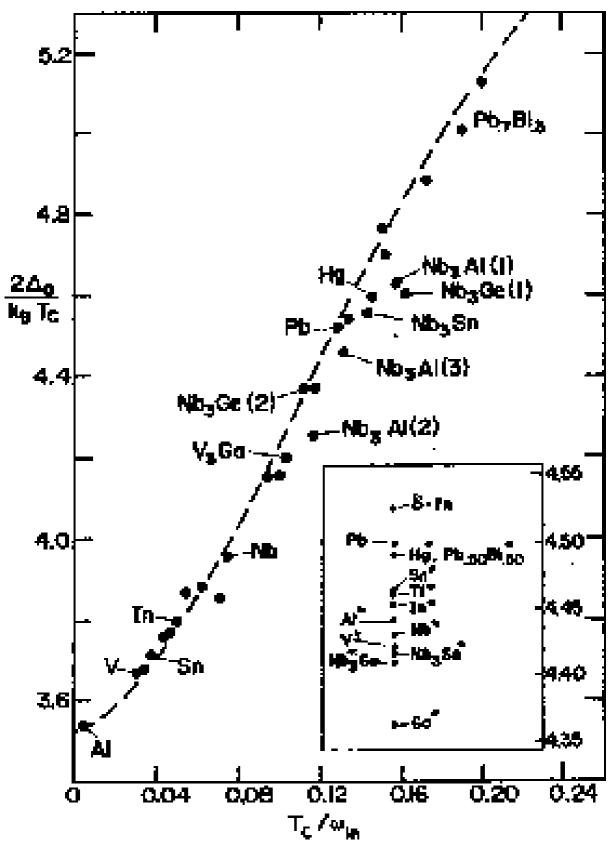
Figure 25: The ratio $2\Delta_{0}/k_{B}T_{c}$ vs $T_{c}/\omega_{\ell n}$. The solid dots represent results from the full numerical solutions of the Eliashberg equations. Experiment tends to agree to within 10%. In increasing order of $T_{c}/\omega_{\ell n}$, the dots correspond to the following systems: $A\ell$, $V$, Ta, Sn, $T\ell$, $T\ell_{0.9}Bi_{0.1}$, In, Nb (Butler), Nb (Arnold), $V_{3}Si(1)$, $V_{3}Si$ (Kihl.), Nb (Rowell), Mo, $Pb_{0.4}T\ell_{0.6}$, La, $V_{3}Ga$, $Nb_{3}A\ell(2)$, $Nb_{3}Ge(2)$, $Pb_{0.6}T\ell_{0.4}$, Pb, $Nb_{3}A\ell(3)$, $Pb_{0.8}T\ell_{0.2}$, Hg, $Nb_{3}Sn$, $Pb_{0.9}Bi_{0.1}$, $Nb_{3}A\ell(1)$, $Nb_{3}Ge(1)$, $Pb_{0.8}Bi_{0.2}$, $Pb_{0.7}Bi_{0.3}$, and $Pb_{0.65}Bi_{0.35}$. The drawn curve corresponds to $2\Delta_{0}/k_{B}T_{c}=3.53[1+12.5(T_{c}/\omega_{\ell n})^{2}\ell n(\omega_{\ell n}/2T_{c})]$. The insert shows results for different scaled $\alpha^{2}F(\omega)$ spectra. They all correspond to the same value of $T_{c}$ and of $\omega_{\ell n}$ as Pb. They serve to show that some deviation from the general trend is possible. Reproduced from Ref. [11].

In obtaining this result the spirit of the McMillan equation was followed, and the coefficients $12.5$ and $2$ were chosen from fits to the numerical data for a large number of superconductors. These results are plotted in Fig. 25. From this Figure it is clear that Eq. (111) describes the overall trend very well. As the electron-phonon interaction increases (i.e. becomes more retarded), the gap ratio increases to values exceeding 5.0.

Figure 25 illustrates that a simple analytic form describes the trend of the gap ratio as a function of ${T_{c}/\omega_{\ln}}$ rather well for a variety of conventional superconductors. In each case electron-phonon spectral functions were used, as obtained from tunneling data, or, in some cases, model calculations. On occasion, one sometimes uses a phonon spectrum obtained from inelastic neutron scattering, scaled to give the measured critical temperature. This latter process assumes that the electron-phonon coupling is constant as a function of frequency (seen to be reasonable in the case of Pb), and often assumes a value of the Coulomb pseudopotential, $\mu^{\ast}(\omega_{c}=6\omega_{\rm max})\approx 0.1$ ($\omega_{\rm max}$ is the maximum phonon frequency). Specific references to the sources of these spectra can be found in Refs. [222, 11].

An important question, particularly when faced with a new superconductor whose phonon characteristics may or may not be ‘typical’, is to what extent the trend modelled by the semi-empirical analytic form, Eq. (111) can be violated, for a given coupling study. This question was considered in Ref. [223]. They took existing electron-phonon spectra, $\alpha_{\circ}^{2}F(\nu)$, and scaled them to new spectra, $\alpha_{\circ}^{2}F(\nu)^{\ast}=B\alpha_{\circ}^{2}F(b\nu)$, where $B$ and $b$ are constants, chosen to span a continuum of values of ${T_{c}/\omega_{\ln}}$. Thus, given some spectral shape, say that of Pb, one can determine a curve of $2\Delta_{\circ}/k_{B}T_{c}$ vs. ${T_{c}/\omega_{\ln}}$. In this way they were able to ascertain, for a given value of ${T_{c}/\omega_{\ln}}$, the shape dependence of the gap ratio. They of course found more significant deviations from the analytical form, Eq. (111); nonetheless, the deviations remained small on the scale of Fig. 25. Larger deviations were obtained with the use of (somewhat artificial) delta-function model spectra [223, 224, 225]. Similarly, if the electron-phonon coupling strength is taken to be extremely high, large deviations occur from one spectral shape to another [226].

The net conclusion is that, with physical spectra and physically relevant coupling strength (${T_{c}/\omega_{\ln}}{<\atop\sim}0.2$), the strong coupling corrections are quasi-universal, and are well described by Eq. (111). We explore in the next subsection how this can be used to optimize the gap and gap ratio.

4.6 Optimal Phonon Spectra and Asymptotic Limits

A functional derivative analysis similar to that described for $T_{c}$ yields, for $\Delta_{\circ}$, an optimum phonon frequency for a given spectral area. One finds that for a delta function spectral function, the zero temperature gap edge obeys a scaling relation just like $T_{c}$ given by Eq. (98):

$$\Delta_{\circ}/A=g({\bar{\omega}}_{E},\mu^{\ast}),$$ (112)

where all quantities are as defined following Eq. (98). As found there, for a given base spectrum, an optimum frequency $\bar{\omega}_{E}^{\ast}$ exists whose value is generally lower than the characteristic frequency of the base spectrum — this is particularly clear when the base spectrum itself is a delta function. With $T_{c}$ one found that shifting the spectral weight to that optimum frequency resulted in an enhancement of $T_{c}$. Furthermore, an iteration of this procedure resulted in convergence to the situation where, for a given spectral area, the maximum $T_{c}$ had been achieved, with a frequency given by $\bar{\omega}_{E}^{\ast}\approx 1.3$ (for $\mu^{\ast}(\omega_{c})=0.1$). The functional derivative of $T_{c}$ with respect to $\alpha^{2}F(\nu)$ using this base spectrum is non-positive definite [199] with a maximum at $\bar{\omega}_{E}^{\ast}$, showing that $T_{c}$ could no longer be increased.

The situation with the gap edge is similar, but differs in the following crucial point. Upon iteration one finds that the optimum frequency continues to decrease, as the Einstein frequency of the base spectrum decreases. Thus, the implication is that the gap edge, and therefore the gapedge ratio, $2\Delta_{\circ}/k_{B}T_{c}$, will be maximized in the limit as $\bar{\omega}_{E}^{\ast}\rightarrow 0$. Alternatively, since these calculations are for fixed spectral area, $A$, this will occur as $\lambda\rightarrow\infty$.

What is the maximum value of $2\Delta_{\circ}/k_{B}T_{c}$ allowed within ‘standard’ Eliashberg theory ? Carbotte et al. [198] answered this question through a scaling theorem, and backed up with numerical work. They found that the gap ratio increased monotonically as $\lambda$ increased, finding (numerically) a value close to 10 (recall BCS gives 3.53) for values of $\lambda\approx 30$. In doing so they proved that $\Delta_{\circ}\propto\sqrt{\lambda}\omega_{E}$ as $\lambda\rightarrow\infty$, just like $T_{c}$ does (Eq. (94)). Claims were made to the contrary, but these were definitively put to rest in Ref. [169]. By solving a set of Eliashberg equations written specifically for $\lambda\rightarrow\infty$, they found a maximum value of the gap ratio equal to 12.7. A variety of other properties were explored in the asymptotic limit, $\lambda\rightarrow\infty$, as can be found in the previous references and in Ref. [227, 228, 229, 230, 231].

5 Thermodynamics and Critical Magnetic Fields

These topics have been amply covered in previous reviews [11]. Nonetheless, we include here for completeness a brief summary of the impact of the electron-phonon interaction on these properties in the superconducting state.

5.1 The Specific Heat

To calculate the specific heat one requires the free energy. For an interacting electron system, a practical formulation of this problem was first proposed by Luttinger and Ward [232], and further pursued by Eliashberg [233]. A simpler calculation requires the free energy difference between the superconducting and normal state, for which an expression due to Bardeen and Stephen [234] is

$${\Delta F\over N(0)}=-\pi T\sum_{m}\biggl{(}\sqrt{\omega_{m}^{2}+\Delta^{2}(i\omega_{m})}-|\omega_{m}|\biggr{)}\biggl{(}Z^{S}(i\omega_{m})-Z^{N}(i\omega_{m}){|\omega_{m}|\over\sqrt{\omega_{m}^{2}+\Delta^{2}(i\omega_{m})}}\biggr{)},$$ (113)

where, for clarity, we include the two Eliashberg equations from Eqs.(54 - 57):

$$Z_{m} = 1+\pi T\sum_{m^{\prime}}\lambda(i\omega_{m}-i\omega_{m^{\prime}}){(\omega_{m^{\prime}}/\omega_{m})Z_{m^{\prime}}\over\sqrt{\omega_{m^{\prime}}^{2}Z^{2}_{m^{\prime}}+\phi^{2}_{m^{\prime}}}}$$ (114)

$$\phi_{m} = \pi T\sum_{m^{\prime}}\biggl{(}\lambda(i\omega_{m}-i\omega_{m^{\prime}})-N(0)V_{\rm coul}\biggr{)}{\phi_{m^{\prime}}\over\sqrt{\omega_{m^{\prime}}^{2}Z^{2}_{m^{\prime}}+\phi^{2}_{m^{\prime}}}}.$$ (115)

These equations ignore band structure effects entirely (except through the electron density of states at the Fermi level, denoted here by $N(0)$), and we again have adopted the shorthand $Z(i\omega_{m})=Z_{m}$ etc., and used the gap function $\Delta(i\omega_{m})\equiv\phi(i\omega_{m})/Z(i\omega_{m})$. For the free energy expression we have used superscripts ‘S’ or ‘N’ to denote the superconducting or normal state, respectively. In the normal state $Z^{N}(i\omega_{m})$ reduces to the expressions obtained in subsection (2.3), which is easily seen if one uses the relation

$$\Sigma(z)=z\bigl{(}1-Z(z)\bigr{)},$$ (116)

where $z$ is a frequency anywhere in the upper half plane, and $\Sigma(z)$ is the electron self-energy.

Equation (113) can easily be evaluated, once the imaginary axis Eliashberg equations (114-115) are solved. From this the specific heat difference,

$$\Delta C(T)=-T{d^{2}\Delta F\over dT^{2}},$$ (117)

and the thermodynamical critical field,

$$H_{c}(T)=\sqrt{-8\pi\Delta F},$$ (118)

can be computed. The former displays a jump at $T_{c}$, characteristic of a mean field theory, which is the level of approximation of Eliashberg theory. At low temperatures the specific heat in the superconducting state should be exponentially suppressed. This is generally observed [141], and deviations that do occur at very low temperatures can readily be explained by anisotropy in the gap parameter [117].

Because properties like the electron density of states at the Fermi level are difficult to measure or calculate reliably, one would like to focus on observables that are independent of these properties. For the specific heat difference, one way of accomplishing this is to normalize the specific heat to the normal state result, which presumably contains the same electron density of states. The result is then independent of $N(0)$, and can be compared directly to the measured results. A textbook example was provided in the case of Al [235]; the data is reproduced in Fig. 26, along with the BCS prediction. The normal state specific heat for a weakly interacting electron gas is given by

$$C_{N}(T)=\gamma T,$$ (119)

where $\gamma$ is the Sommerfeld constant given by

$$\gamma={2\over 3}\pi^{2}k_{B}^{2}N(0)(1+\lambda).$$ (120)

Here, $\lambda$ is the electron-phonon enhancement parameter, already referred to on many occasions. The electron-phonon interaction alters the low temperature specific heat through the mass enhancement parameter, $1+\lambda$. In fact, a more careful treatment [100, 236, 88] yields a temperature-dependent $\gamma(T)$ for the specific heat coefficient (which, at very low temperature, reduces to the Sommerfeld $\gamma$). Besides providing quantitative corrections to the electronic specific heat in the normal state, this correction also provides a properly physical contribution from the low frequency phonon modes, as found in Ref. [237].

For a variety of conventional superconductors, like Al, the normal state low temperature specific heat is easily measured by suppressing the superconducting state with a magnetic field. Then the ratio $\Delta C(T)/\gamma T_{c}$ can be determined. At $T_{c}$, the BCS result for this ratio is universal, like the gap ratio: it is 1.43. Strong coupling corrections can be derived [221] as before, as a function of the strong coupling parameter, $T_{c}/\omega_{\ln}$. The result is

$${\Delta C(T_{c})\over\gamma T_{c}}=1.43\biggl{[}1+53\bigl{(}{T_{c}\over\omega_{\ln}}\bigr{)}^{2}\ln{({\omega_{\ln}\over 3T_{c}})}\biggr{]}.$$ (121)

Again, the coefficients $53$ and $3$ were determined semi-empirically by fits to numerical data. A plot of this result, along with some of the numerical data, is shown in Fig. 27. We already remarked about Al — its calculated value is indicated by the point nearest the ordinate, and agrees very well with experiment. The result for Pb is also shown; the experimental value is 2.65, almost a factor of 2 greater than the BCS result. The theoretical result, based on a numerical solution of Eqs. (113-115), is in good agreement.

The result for stronger coupling has also been calculated [226]. In particular, the asymptotic limit can be computed, following standard procedures. The result is [229]

$${\Delta C(T_{c})\over\gamma T_{c}}={19.9\over\lambda},$$ (122)

showing that the relative magnitude of the jump decreases for large $\lambda$, and therefore, as is already becoming apparent in Fig. 27, the specific heat will have a maximum as a function of coupling strength.

Similar results can be derived for other thermodynamic properties as well. These have been summarized in Ref. [11] and will be omitted here.

5.2 Critical Magnetic Fields

In a type-I superconductor, a critical magnetic field ($H_{c}$) exists, given by Eq. (118). In a type-II superconductor, a lower critical field, $H_{c1}$, and an upper critical field, $H_{c2}$, exist; the former signals the departure from the Meissner state to one in which one vortex penetrates the system, while the latter occurs at the normal/superconducting transition. The thermodynamic critical field continues to exist as a thermodynamic property, but not one that can be measured by application of a magnetic field.

A theory of $H_{c1}$ has been worked out within the BCS approximation in Ref. [238, 239] (in the dirty limit). This work was extended to the level of Eliashberg theory in Ref. [240]. It is traditional to calculate the reduced field, $h_{c1}(T/T_{c})\equiv{H_{c1}(T)\over T_{c}H^{\prime}_{c1}(T_{c})}$ as a function of $T/T_{c}$. Such a curve has a slope of $-1$ near $T_{c}$, and saturates to some value at $T=0$. Rammer [240] found that the low temperature value decreased with coupling strength (there characterized by a particular spectrum).

A detailed theory has also been provided for the upper critical field, $H_{c2}$. In 1957 Abrikosov essentially created the subject of type II superconductivity [241]. Both experimental and theoretical work in this exciting area continued to flourish throughout the 1960’s. Applications of superconductivity in the mixed state require type II superconductivity in order to sustain high magnetic fields. Abrikosov’s solution used the phenomenology of Ginzburg-Landau theory [45]. Further theoretical developments utilized the microscopic theory of Gor’kov [44]. The first of these was by Gor’kov [242] for clean superconductors, followed by five papers by Werthamer and collaborators to include impurity effects [243, 244], spin and spin-orbit effects [245], Fermi surface anisotropy effects [246], and retardation effects [247]. All of these papers used an instantaneous attractive potential (i.e. as in BCS theory), except for the last. Further developments to include retardation effects were carried out in Refs. [248, 238, 138, 139] and others. Finally, in Ref. [249] the Eliashberg theory of $H_{c2}$, including Pauli paramganetic limiting and arbitrary impurity scattering, was formulated and solved.

Without retardation effects or Pauli limiting, the zero temperature upper critical field, when expressed in terms of the slope near $T_{c}$, takes on universal values, dependent only on the elastic impurity scattering rate, given by $1/\tau$. For example, the quantity $h_{c2}(0)\equiv H_{c2}(0)/(T_{c}|H^{\prime}_{c2}(T_{c})|)$ is given by 0.693 in the dirty limit ($1/\tau>>\Delta$) and 0.727 in the clean limit ($1/\tau=0$). For intermediate scattering rates the result falls somewhere in between. It is worth mentioning that the absolute value of the upper critical field increases with increased impurity scattering. We often use the ratio because the slope near $T_{c}$ is measured, and then the zero temperature value is obtained by using the universal number quoted above. The value at zero temperature is of special interest because the Ginzburg-Landau coherence length can then be extracted through

$$H_{c2}={\Phi_{0}\over 2\pi\xi_{\rm GL}^{2}}.$$ (123)

Here $\Phi_{0}$ is the fluxoid quantum, and we have used the subscript ‘GL’ to denote the Ginzburg-Landau coherence length, which, at zero temperature, is often close to the BCS coherence length, and gives us an indication of the Cooper pair size [250]. Hence, deviations from 0.693 (or 0.727) due to retardation effects are of interest for this reason.

For completeness, we quote the equations which govern $H_{c2}$, taking into account electron-phonon interactions in the Eliashberg sense, and Pauli limiting. The gap equation is linear in the order parameter [249]

$$\tilde{\Delta}(i\omega_{n})=\pi T\sum_{m}\biggl{[}\lambda(i\omega_{n}-i\omega_{m})-\mu^{\ast}\biggr{]}{\tilde{\Delta}(i\omega_{m})\over\chi^{-1}(\tilde{\omega}(i\omega_{m}))-1/2\tau},$$ (124)

with

$$\tilde{\omega}(i\omega_{n})=\omega_{n}+\pi T\sum_{m}\lambda(i\omega_{n}-i\omega_{m}){\rm sgn}\omega_{m}+{1\over 2\tau}{\rm sgn}\omega_{n}.$$ (125)

The factor $\chi(\tilde{\omega}(i\omega_{n}))$ is given by

$$\chi(\tilde{\omega}(i\omega_{n}))={2\over\sqrt{\alpha}}\int_{0}^{\infty}dq\,e^{-q^{2}}{\rm tan}^{-1}\bigl{(}{\sqrt{\alpha}q\over|\tilde{\omega}(i\omega_{n})|+i\mu_{B}H_{c2}{\rm sgn}\tilde{\omega}(i\omega_{n})}\bigr{)}.$$ (126)

Here $\alpha(T)\equiv{1\over 2}|e|H_{c2}(T)v_{F}^{2}$, with $e$ the charge of the electron and $v_{F}$ the electron Fermi velocity. $\mu_{B}$ is the Bohr magneton. Eq. (124) can be written as an eigenvalue equation, just like $T_{c}$. It is linear because the solution is valid only on the phase boundary between the normal and the superconducting states.

We have carried out extensive numerical investigations of $h_{c2}(0)$ as a function of coupling strength. In the conventional regime, the dependence on coupling strength is very weak [251]; in the dirty limit $h_{c2}(0)$ decreases initially (as a function of $T_{c}/\omega_{\ln}$) to about 0.65, and then increases to beyond 0.70. In the clean limit there is first a barely discernible decrease, followed by an increase to values of approximately 0.80. These are all theoretical results, and, in many cases have not been carefully investigated with experiment. On the other hand the expected changes are of order 10% or less, and may well be masked by other effects. A thorough investigation was provided for Nb by Schachinger et al. [252]. The agreement with the available data was excellent (although they did invoke, in addition to the theoretical framework described here, anisotropy effects). For further information the interested reader is directed to the aforementioned references.

Before leaving this section we should also mention that optimum spectrum analysis [201] and asymptotic limits (3rd reference in [229]) have also been investigated for $H_{c2}$; the result is very dependent on elastic impurity content, except in the asymptotic limit. In that case, the results approach a universal value, i.e. $h_{c2}(0)\rightarrow 0.57$ as $\lambda$ increases.

6 Response Functions

In the previous sections we have seen effects due to the inclusion (through the Eliashberg formalism) of the detailed electron-phonon coupling. The result is in many cases a large quantitative correction to the corresponding BCS result. In this way one can infer, from experiment, the necessity of taking into account the dynamics of the electron-phonon interaction. Nonetheless, as we saw in Section 3 (particularly in the Tunneling and Optical Conductivity subsections) dynamical interactions manifest themselves more clearly in dynamical properties. For this reason we now focus on various response functions.

6.1 Formalities

A theory of linear response can be approached from two very different frameworks, the Kubo formalism, and the Boltzmann equation. The two frameworks often lead to the same result; their connection is discussed at length in Ref. [83]. Early treatments [5, 253] of the various response functions in a superconductor neglected the electron-phonon interaction, except insofar as it provided the mechanism for the superconductivity in the first place. The main interest was the investigation of a new state which apparently had a single electron energy gap, which would manifest itself either directly in spectroscopic methods (optical and tunneling) or more indirectly as a function of temperature (NMR relaxation rate, acoustic attenuation, etc.). Sometime later two seminal papers appeared [254, 100], both of which discussed the impact of the electron-phonon interaction on transport in the electron gas. These dealt specifically with the normal state. Work at a similar level but in the superconducting state appeared a little later [255]; this latter work was generalized to apply for arbitrary elastic impurity scattering only much later [256]. These authors used quasiclassical techniques; below we will sketch an alternative derivation based on the Kubo [257] formula.

We should preface this work with some remarks about vertex corrections. They are generally ignored in calculations of response functions, so that a particle-hole ‘bubble’, consisting of one single electron Green function and one single hole Green function, requires evaluation [258]. Older work [263, 264] investigated the need for vertex corrections and found that they contributed very little; later work in the normal state [182, 176] suggested that their contribution could be summarized by substituting a ‘transport’ electron-phonon spectral function, $\alpha_{\rm tr}^{2}F(\nu)$, for the usual spectral function, $\alpha^{2}F(\nu)$, in the transport equations. This alteration discriminated in favour of back scattering as being particularly effective in depleting the current, as one would expect. Over a large frequency range, however, these spectral functions are not expected to differ substantially; nonetheless, quantitative investigations are currently lacking [83], particularly in the superconducting state.

The contribution to the conductivity consists of two components: the paramagnetic and diamagnetic responses. The diamagnetic response is straightforward [265]; the paramagnetic response is determined by the evaluation of a current-current response function. A standard decoupling of this function (ignoring, as noted above, vertex corrections) yields

$$\sigma(\nu)={i\over\nu+i\delta}\Bigl{(}\Pi(\nu+i\delta)+{ne^{2}\over m}\Bigr{)},$$ (127)

where $\Pi(\nu+i\delta)$ is the paramagnetic response function whose frequency dependence (on the imaginary frequency axis) is given by

$$\Pi(i\nu_{n})={1\over N\beta}\sum_{{\bf k},m}{\rm Tr}(ev_{x})^{2}\hat{G}({\bf k},i\omega_{m})\hat{G}({\bf k},i\omega_{m}+i\nu_{n}),$$ (128)

where $\hat{G}({\bf k},i\omega_{m})$ is actually a matrix in the Nambu formalism [2]. It is given, in terms of functions with which we are already familiar, by

$$\hat{G}({\bf k},i\omega_{m})=-{i\omega_{m}Z(i\omega_{m})+(\epsilon_{\bf k}-\mu)\hat{\tau}_{3}+\phi(i\omega_{m})\hat{\tau}_{1}\over(\epsilon_{\bf k}-\mu)^{2}-(i\omega_{m}Z(i\omega_{m}))^{2}+\phi^{2}(i\omega_{m})},$$ (129)

where the Pauli spin matrices are given by

$$\hat{\tau}_{0}\equiv\left(\matrix{1&0\cr 0&1\cr}\right),\,\,\,\,\hat{\tau}_{1}\equiv\left(\matrix{0&1\cr 1&0\cr}\right),\,\,\,\,\hat{\tau}_{2}\equiv\left(\matrix{0&-i\cr i&0\cr}\right),\,\,\,\,\hat{\tau}_{3}\equiv\left(\matrix{1&0\cr 0&-1\cr}\right).$$ (130)

In Eq. (128) the trace is over the Pauli spin space. The presence of the factor $(ev_{x})^{2}$ shows explicitly that the dressed vertex has been replaced with a bare vertex; $v_{x}$ is the component of the electron velocity in the x-direction. The momentum sum is over the entire Brillouin zone; the factors preceding the summations include the total number of atoms in the crystal, $N$, and the inverse temperature, $\beta\equiv 1/k_{B}T$. The diamagnetic piece in Eq. (127) contains the electron density $n$ and the electron mass, $m$. Finally, the single electron energy is denoted by $\epsilon_{\bf k}$, and, as before, we use a notation where we explicitly subtract off the chemical potential, $\mu$.

The paramagnetic kernel denoted by $\Pi(i\nu_{n})$ in Eq. (128) is a special case of a more general ‘bubble’ diagram. A similar calculation, for example, is required for the NMR relaxation rate [266, 168, 267], or the phonon self-energy [268, 269, 270, 271], except that the vertices are not proportional to $\hat{\tau}_{0}$ (as was the case in Eq. (128)), but to some other Pauli matrix. This has the effect that the so-called ‘coherence factors’ will differ, depending on the particular response function; some will result in a cancellation with singularities arising from the single electron density of states, whereas others will result in a potentially singular response, at low frequencies, as we shall see below. An early review outlining these differences in the context of Eliashberg theory is given in Ref. [14].

Returning to Eq. (128), the standard procedure is as follows; one would like to evaluate the Matsubara sum — only then can one perform the proper analytic continuation to real frequencies required for the optical conductivity. This is straightforward, through the spectral representation, which is the Nambu generalization of Eq. (26). The cost is that two new frequency integrals are required, one of which can be done immediately by making use of the Kramers-Kronig-like relation (see Eq. (68))

$$\hat{G}({\bf k},z)=\int_{-\infty}^{\infty}\,d\omega{\hat{A}({\bf k},\omega)\over z-\omega},$$ (131)

with $z$ anywhere in the upper half plane. Finally, we would like to perform the Brillouin zone integration analytically; to do so, we note that the only dependence on wavevector ${\bf k}$ in Eq. (128) occurs through $\epsilon_{\bf k}$ (this is not so for more complicated response functions, such as is required for neutron scattering, for example, where the momentum dependent kernel, $\Pi({\bf q},\nu+i\delta)$, is required). This feature of the optical response allows us to make the usual replacement, given already by Eq. (18):

$${1\over N}\sum_{\bf k}\rightarrow\int\,d\epsilon N(\epsilon),\\$$

where $N(\epsilon)$ is the single electron density of states. As in that case $N(\epsilon)$ can be taken as constant ($=N(\epsilon_{F})$) and, along with the electron velocity, $v_{x}$, taken out of the integration as an overall constant, $2N(\epsilon_{F})e^{2}v_{x}^{2}\equiv{\omega_{P}^{2}\over 4\pi}\equiv ne^{2}/m$, where $\omega_{P}$ is the electron plasma frequency. However, one would normally like to extend the integration over single electron energy from $-\infty$ to $+\infty$, as is often done within Eliashberg theory. Here, however, one has to be slightly more careful, and first subtract the normal state contribution to the kernel. This makes the integral sufficiently convergent that extension to an infinite bandwidth (effectively) is possible. Then the integral can be readily performed by contour integration. The integration over the normal state contribution alone must be done separately; an integration cutoff $\pm D$ must be used, the effect of which is an additional (imaginary) contribution. The final result is [272]

$$\sigma(\nu) = {ine^{2}\over m\nu}\Biggl{\{}\int_{0}^{\infty}d\omega\tanh({\beta\omega\over 2})\Bigl{(}h_{1}(\omega,\omega+\nu)-h_{2}(\omega,\omega+\nu)\Bigr{)}$$ (132)

$$\phantom{{ne^{2}\over m}\Biggl{\{}-1}+\int_{-\nu}^{D}d\omega\tanh({\beta(\omega+\nu)\over 2})\Bigl{(}h_{1}^{\ast}(\omega,\omega+\nu)+h_{2}(\omega,\omega+\nu)\Bigr{)}\Biggr{\}}$$

with

$$h_{1}(\omega_{1},\omega_{2}) = {1-N(\omega_{1})N(\omega_{2})-P(\omega_{1})P(\omega_{2})\over 2(\epsilon(\omega_{1})+\epsilon(\omega_{2}))}$$

$$h_{2}(\omega_{1},\omega_{2}) = {1+N^{\ast}(\omega_{1})N(\omega_{2})+P^{\ast}(\omega_{1})P(\omega_{2})\over 2(\epsilon(\omega_{2})-\epsilon^{\ast}(\omega_{1}))}$$

$$N(\omega) = {\tilde{\omega}(\omega+i\delta)\over\epsilon(\omega+i\delta)}$$

$$P(\omega) = {\phi(\omega+i\delta)\over\epsilon(\omega+i\delta)}$$

$$\epsilon(\omega) = \sqrt{\tilde{\omega}^{2}(\omega+i\delta)-\phi^{2}(\omega+i\delta)}$$ (133)

where $D$ is the large cutoff mentioned above, to be taken to infinity for large electronic bandwidth, and $\tilde{\omega}(\omega+i\delta)\equiv\omega Z(\omega+i\delta)$.

Various limits can be extracted from these expressions; for example the normal state results of Section 3.3.3 can be readily obtained, as well as the simple Drude result, obtained by assuming only elastic scattering characterized by a frequency independent rate, $1/\tau$. When inelastic scattering is included (here through electron-phonon scattering), low frequency Drude-like fits can be obtained through simple expansions [184]. We will turn to these later.

Equation (132) represents the ‘standard’ theory of the optical conductivity with Eliashberg theory. As already mentioned, this characterization includes the caveats discussed above about vertex corrections and $\alpha^{2}F(\nu)\rightarrow\alpha_{\rm tr}^{2}F(\nu)$ replacements. It is valid for both inelastic scattering and elastic scattering processes (within the Born approximation). The impact of elastic scattering on the Eliashberg equations have not yet been discussed, so we turn to these now. Equations (114,115), on the imaginary axis, along with Eqs. (73,74), on the real frequency axis, are written for the clean limit (‘clean limit’ is here defined to mean that the elastic scattering rate is zero, $1/\tau=0$). When elastic scattering is included, new terms appear on the right hand side of these equations. (As an aside, one way of using the existing equations to include elastic scattering is to include a component of $\alpha^{2}F(\nu)$ (called $\alpha_{\rm imp}^{2}F(\nu)$ for simplicity) which models the elastic scattering part. At any non-zero temperature it will be given by a zero frequency contribution

$$\alpha_{\rm imp}^{2}F(\nu)={\nu\over 2\pi\tau T}\delta(\nu).$$ (134)

Substitution of this expression into Eqs. (114,115), for example, will yield simple expressions on the right hand side proportional to $1/\tau$.) In principle one would think that Eqs. (114,115,73,74) require iteration to a solution for every new value of impurity scattering. In actual fact, however, they need be solved only in the clean limit. Then, the pairing $\phi(\omega+i\delta)$, and renormalization $\tilde{\omega}(\omega+i\delta)\equiv\omega Z(\omega+i\delta)$ functions can be modified by the simple contribution

$$\phi(\omega+i\delta)\rightarrow\phi(\omega+i\delta)+{i\over 2\tau}{\phi(\omega+i\delta)\over\sqrt{\tilde{\omega}^{2}(\omega+i\delta)-\phi^{2}(\omega+i\delta)}}$$ (135)

$$\tilde{\omega}(\omega+i\delta)\rightarrow\tilde{\omega}(\omega+i\delta)+{i\over 2\tau}{\tilde{\omega}(\omega+i\delta)\over\sqrt{\tilde{\omega}^{2}(\omega+i\delta)-\phi^{2}(\omega+i\delta)}}.$$ (136)

Equations (132,133) remain the same with impurity scattering. This is a consequence of the so-called Anderson’s ‘theorem’ [121]. The modifications are all implicitly contained in the pairing and renormalization functions. Note that the gap parameter, $\Delta(\omega+i\delta)\equiv\phi(\omega+i\delta)\bigg{/}Z(\omega+i\delta)$, remains the same, independent of the impurity scattering rate.

6.2 BCS results

The purpose of this chapter is to examine effects specifically due to the electron-phonon interaction. Nonetheless, it is best to first see what occurs in the BCS limit, and then examine the differences. The means for achieving the BCS limit from Eliashberg theory was examined in Section 4.1; in general we mean by the ‘BCS limit’ that limit which corresponds to taking $\alpha^{2}F(\nu)$ to be non-zero only for some very high frequency component (so that the “strong coupling” indicator $T_{c}/\omega_{\ln}\rightarrow 0$). As a result, the renormalization function, $Z(\omega+i\delta)\rightarrow 1$, and the gap function $\Delta(\omega+i\delta)\rightarrow\Delta$, a constant, as a function of frequency. This allows one to explicitly break up the integrals in Eq. (132) into portions involving the BCS gap parameter, $\Delta$, and the electromagnetic frequency, $\nu$. A very efficient FORTRAN program has been provided in Ref. [273] in this case.

6.2.1 Far-Infrared: Dirty Limit

A historically important case is the dirty limit. This is defined by $1/\tau>>\Delta$, and was first treated by Mattis and Bardeen [253]. An analytical expression can be obtained at zero temperature [253]:

$${\sigma_{1}\over\sigma_{n}} = \bigl{(}1+{2\Delta\over\nu}\bigr{)}E(k)-{4\Delta\over\nu}K(k)\,\,\,\,\,\,\,\,\nu>2\Delta$$ (137)

$${\sigma_{2}\over\sigma_{n}} = {1\over 2}\bigl{(}1+{2\Delta\over\nu}\bigr{)}E(k^{\prime})-{1\over 2}\bigl{(}1-{2\Delta\over\nu}\bigr{)}K(k^{\prime}),$$ (138)

where $\sigma_{n}\equiv{ne^{2}\tau\over m}$ is the normal state conductivity (pure real) and the real part of the conductivity is identically zero for frequencies, $\nu<2\Delta$. In these expressions

$$k=|{2\Delta-\nu\over 2\Delta+\nu}|\,\,\,\,\,{\rm and}\,\,\,\,\,\,k^{\prime}=\sqrt{1-k^{2}},$$ (139)

and $E(k)$ and $K(k)$ are the complete elliptic integrals of the first and second kind. For other cases (finite temperature and/or lower impurity scattering rate) one must integrate numerically [273]. Figure 28 shows (a) the real part and (b) the imaginary part of the conductivity in the zero temperature BCS superconducting state, for various impurity scattering rates. We have used some definite values for the impurity scattering rates and the coupling strength. The latter has been chosen to yield an absorption edge, $2\Delta=10.4$ meV, which, because of the insensitivity of superconductivity to elastic impurity scattering [121], holds for all scattering rates. A well-defined absorption onset is evident in Fig. (28a); otherwise the curves simply deviate from what would have been Drude-like curves in the normal state. In Fig. (28b) the frequency times the imaginary part of the conductivity is shown for the same scattering rates. Such a combination is shown because the zero frequency limit gives a direct measure of the London penetration depth:

$$1/\lambda^{2}(T)=\lim_{\nu\rightarrow 0}{4\pi\over c^{2}}\nu\sigma_{2}(\nu).$$ (140)

As is evident from the figure, the penetration depth increases as the impurity scattering rate increases.

Another feature stands out in Fig. (28b); there is a notable ‘dip’ in $\nu\sigma_{2}(\nu)$ at $2\Delta$, particularly in the clean limit. Otherwise the curves all approach the Drude limit at high frequency, which, for this property, is unity (conductivities are in units of $ne^{2}/m\equiv\omega_{P}^{2}/4\pi$).

6.2.2 Penetration Depth

Before we examine the effects of the electron phonon interaction on the real and imaginary parts of the conductivity, we first summarize the ‘BCS’ results for the penetration depth as a function of impurity scattering, which can be extracted analytically [274, 186] from the zero frequency limit of the conductivity. The result is, with $\alpha\equiv{1\over 2\Delta\tau}$,

$${1\over\lambda^{2}(T=0)} = {1\over\lambda_{cl}^{2}(T=0)}\Biggl{\{}{\pi\over 2\alpha}-{1\over\alpha\sqrt{1-\alpha^{2}}}\sin^{-1}(\sqrt{1-\alpha^{2}})\Biggr{\}}\phantom{bbbbbbbbbb}\alpha<1$$ (141)

$${1\over\lambda_{cl}^{2}(T=0)}\Biggl{\{}{\pi\over 2\alpha}-{1\over 2\alpha\sqrt{\alpha^{2}-1}}\ln\Bigl{(}{\alpha+\sqrt{\alpha^{2}-1}\over a-\sqrt{\alpha^{2}-1}}\Bigr{)}\Biggr{\}}\phantom{bbbbbb}\alpha>1.$$

Here, the zero temperature London penetration depth in the clean limit is given by

$$\lambda_{cl}^{2}(T=0)={mc^{2}\over 4\pi ne^{2}}.$$ (142)

In the weak scattering limit Eq. (141) reduces to the more familiar form,

$${1\over\lambda^{2}(0)}\approx{1\over\lambda_{cl}^{2}(0)}{1\over 1+{\pi\over 4}\alpha}.$$ (143)

This expression can be written in terms of the zero temperature coherence length, $\xi_{0}$, and the mean free path, $\ell$, using $\Delta={v_{F}\over\pi\xi_{0}}$ and $v_{F}=\ell/\tau$, where $v_{F}$ is the Fermi velocity:

$${1\over\lambda^{2}(0)}\approx{1\over\lambda_{cl}^{2}(0)}{1\over 1+{\pi^{2}\over 8}{\xi_{0}\over\ell}}.$$ (144)

6.2.3 Microwave Regime: Coherence Factors

The microwave regime (1 - 60 GHz) corresponds to very low energies (1 GHz = 0.0041 meV). This energy scale is much lower than that of the superconducting energy gap. Measurements of the microwave response of a superconductor have been used in recent years to determine the penetration depth and optical conductivity in the high $T_{c}$ cuprates [275, 276], but, historically, either the real or the imaginary component of the surface impedance was measured, making a determination of the complex conductivity impossible. It is of interest to examine the conductivity in this case, because BCS theory makes a highly non-trivial prediction that the real part of the conductivity shows a so-called coherence peak just below $T_{c}$. This coherence peak was almost simultaneously predicted [5] and observed [277, 278] in measurements of the NMR relaxation rate [279]. We will briefly discuss the source of these coherence factors, and return to a description of the microwave conductivity, since a detailed discussion of the NMR relaxation rate [281] is outside the scope of this review, and the final expression relevant to superconductors is a special case of the microwave conductivity.

Within BCS theory the transition probabilities between an initial and final state that enter the expression for various linear response functions are of the form [5, 46]

$$F_{\bf kk^{\prime}}=(u_{\bf k}u_{\bf k^{\prime}}\mp v_{\bf k}v_{\bf k^{\prime}})^{2}$$ (145)

with $u_{\bf k},v_{\bf k}$ the amplitudes that relate quasiparticle operators to electron operators

$$u_{\bf k}=\left({1\over 2}\left(1+{\epsilon_{\bf k}-\mu\over E_{\bf k}}\right)\right)^{1/2}$$ (146)

$$v_{\bf k}=\left({1\over 2}\left(1-{\epsilon_{\bf k}-\mu\over E_{\bf k}}\right)\right)^{1/2}$$ (147)

and $E_{\bf k}$ is the usual quasiparticle energy:

$$E_{\bf k}=\sqrt{(\epsilon_{\bf k}-\mu)^{2}+\Delta_{\bf k}^{2}}$$ (148)

where $\epsilon_{\bf k}$ is the electron band energy, $\mu$ is the chemical potential and $\Delta_{\bf k}$ is the gap function. In Eq. (145) the upper (lower) sign corresponds to case I (case II) observables. These signs have important consequences for the response, particularly just below $T_{c}$. A case in point is the electromagnetic absorption; the temperature-dependent result (derived from Eqs. (132,133)) in the dirty limit ($1/\tau>>\Delta$) is [253]

$${\sigma_{1}\over\sigma_{n}} = {2\over\nu}\int^{\infty}_{\Delta_{0}}dE{E(E+\nu)+\Delta_{0}^{2}\over(E^{2}-\Delta_{0}^{2})^{1/2}((E+\nu)^{2}-\Delta_{0}^{2})^{1/2}}[f(E)-f(E+\nu)]$$ (149)

$$+ \theta(\nu-2\Delta_{0}){1\over\nu}\int^{-\Delta_{0}}_{\Delta_{0}-\nu}dE{E(E+\nu)+\Delta_{0}^{2}\over(E^{2}-\Delta_{0}^{2})^{1/2}((E+\nu)^{2}-\Delta_{0}^{2})}[1-2f(E+\nu)],$$

where $\Delta_{0}\equiv\Delta(T)$ is the temperature-dependent gap function. The second plus sign in $E(E+\nu)+\Delta_{0}$ which appears in this expression is due to the fact that the electromagnetic absorption is a case II observable. In a case I observable this would be a minus sign; it is then readily seen that whereas Eq. (149) contains a divergence as $\nu\rightarrow 0$, the corresponding case I observable would not, as the numerator (coming from the coherence factor given in Eq. (145)) would then cancel the density of states factors, which are explicit in Eq. (149), and which contain square-root divergences. In both cases the ‘freezing out’ of excitations as the temperature is reduced leads to a low temperature suppression of the response function — this is simply a consequence of the gap. On the other hand, near $T_{c}$ an enhancement is expected for type II observables, while, for type I observables, the response is immediately suppressed as the temperature is lowered below the superconducting transition temperature. In the limit that the frequency is zero, one obtains from Eq. (149),

$${\sigma_{1}\over\sigma_{n}}=2\int^{\infty}_{\Delta_{0}}dE{E^{2}+\Delta_{0}^{2}\over E^{2}-\Delta_{0}^{2}}\bigl{(}-{\partial f\over\partial E}\bigr{)}\equiv(1/T_{1})_{s}/(1/T_{1})_{n},$$ (150)

which is formally divergent (at all temperatures). The divergence is in fact eliminated in practice by anisotropy in the gap or retardation effects. As noted by the second equality, this is the expression for the superconducting to normal ratio of the NMR relaxation rate.

For a type I observable (like the ultrasonic attenuation) the numerator in Eq. (150) has a minus sign, so that numerator and denominator cancel, and the remaining integral is trivial. One obtains

$$\alpha_{s}/\alpha_{n}=2f(\Delta(T)),$$ (151)

where $\alpha_{s(n)}$ is the ultrasonic attenuation in the superconducting (normal) state, and $f$ is the Fermi function. This is a monotonically decreasing function as the temperature decreases from $T_{c}$ to zero.

6.2.4 Far-Infrared Regime — Arbitrary Impurity Scattering

The expressions for the optical conductivity provided in the last three subsections apply only in the dirty limit. As already mentioned earlier, a comprehensive expression (for all values of elastic impurity scattering), along with a very efficient FORTRAN program, was provided in Ref. [273]. For completeness, we illustrate here the temperature dependence for two extreme cases, close to the clean limit ($1/\tau=1$ meV), and the dirty limit ($1/\tau\rightarrow\infty$), in Fig. 29 and Fig. 30, respectively. As noted earlier, the optical gap ($=2\Delta(T)$) is clearly evident in both the real and imaginary part of the conductivity. The evolution from the normal state to the superconducting state is clearly evident as well; note, in particular, that in the real part of the conductivity, the missing area is taken up as a delta function at the origin (not shown).

6.3 Eliashberg Results

Within Eliashberg theory, changes occur for two related reasons. First, even in the normal state the self-energy acquires a frequency dependence (no wavevector dependence, because of the simplifying assumptions made at the start); secondly, the gap function in the superconducting state acquires a frequency dependence and acquires an imaginary part. This latter fact tends to smear many of the ‘sharp’ results shown in the last section, a feature which is already evident in comparing the single electron densities of states in Fig. (24) to those in Fig. (21b), for example. For this reason, it is important to re-examine the impact of retardation on a variety of observables.

6.3.1 NMR Relaxation Rate

In the first few years following the discovery of the high temperature superconductors [8], several anomalous features were measured in the superconducting state. One of these was the absence of the coherence peak (the so-called ‘Hebel-Slichter’ peak) in the NMR spin relaxation rate, $1/T_{1}$, just below $T_{c}$ [282]. Motivated by the possibility that this ‘anomaly’ could be explained by damping effects due to retardation, Allen and Rainer [168] and Akis and Carbotte [267] calculated the ratio of the relaxation rate in the superconducting state to that in the normal state with several hypothetical electron-phonon spectra (obtained by scaling known spectra from conventional superconductors). Both groups found that sufficiently strong coupling (as measured by $\lambda$ or $T_{c}/\omega_{\ln}$) smears out the coherence peak entirely. An example is shown in Fig. 31 (taken from Ref. [168]), which shows the theoretical and experimental [283] results for a conventional superconductor (Indium) along with data from YBCO [284], and theoretical results obtained using scaled spectra. While the present consensus is that the lack of a coherence peak is not solely due to damping effects, the lesson learned from these calculations is clear: retardation effects damp out the coherence peak in the NMR relaxation rate. It is worth noting here that even within a BCS framework (i.e. no retardation), the coherence peak can be suppressed in the dilute electron density limit [285].

6.3.2 Microwave Conductivity

A natural extension of this argument applies to the microwave conductivity. In this case, even within BCS theory, a divergence does not occur since the experiment is conducted at some definite non-zero microwave frequency (see Eq. (149)). Before discussing retardation effects, however, it is important to realize the amount of impurity scattering (as characterized by $1/\tau$) also influences the height and presence of the coherence peak [260, 261]. In Fig. (32a) we show, within the BCS framework, the conductivity ratio for a small but finite frequency as a function of reduced temperature, for a variety of elastic scattering rates, ranging from the dirty limit to the clean limit. Quite clearly the coherence peak is reduced and then eliminated as a function of $1/\tau$.

To see how retardation effects also serve to reduce and eliminate the coherence peak (just as in NMR) we focus on the dirty limit ($1/\tau\rightarrow\infty$) where the peak is largest without retardation. In Fig. (32b) we show results obtained from a Pb spectrum (Fig. 11), scaled by varying degrees to increase $\lambda$ from 0.77 to 3.1. For the largest coupling considered the coherence peak has essentially vanished. This is the same effect seen in the NMR relaxation rate. In Fig. (32c) we illustrate the impact of changing the microwave frequency. Clearly, in the limit of very weak coupling (BCS) one expects the strongest variation, since, as $\nu\rightarrow 0$, the BCS result will diverge logarithmicly. However, as the coupling strength increases, the damping due to retardation reduces the peak far more effectively than an increase in microwave frequency would, so that the conductivity ratio (at some temperature near where a maximum would occur in the BCS limit) is essentially constant as a function of frequency. This is clearly illustrated by the two lowest curves in the Figure, representing the strongest coupling situations.

A measurement of the coherence peak in the microwave wasn’t actually performed until the early 1990’s, in Pb [286] and in YBCO [287] (although the peaks observed in these latter measurements are now thought not to be the BCS coherence peak [288, 289, 276].

Several other groups have since examined the microwave response in conventional superconductors. In Ref. [290] Nb was examined in detail. The experiment was performed at 17 GHz, and a prominent coherence peak was observed, as shown in Fig. 33. Also shown are theoretical curves obtained from Eliashberg calculations; they all fall significantly below the experimental results. We have also included the BCS result (dotted curve) computed for this frequency; it is not very different from one of the curves obtained using the full Eliashberg formalism. The BCS result represents probably the highest achievable coherence peak; other alterations of the standard theory (anisotropy, finite bands, non-dirty limit, etc.) would tend to decrease the theoretical result further. Hence, at present the coherence peak observed in Nb remains anomalous because it is too big. Other measurements in Nb and Pb [291] showed agreement with Eliashberg theory, but they were carried out at a much higher frequency (60 GHz). Another measurement of the electrodynamic response (using simultaneous measurement of the amplitude and phase of the transmission in Nb thin films) [292] supported our results. A more recent measurement of the coherence peak in Nb₃Sn [293] also finds a large discrepancy with Eliashberg theory — the experimental results show a peak which is far too large compared to theory.

6.3.3 Far-Infrared Regime

While more recent investigations of the far-infrared (and slightly lower Terahertz) regime in superconductors utilize transmission techniques which simultaneously measure amplitude and phase information [288, 292], the more conventional Fourier-transform spectroscopy [180] requires Kramers-Kronig relations, as outlined in Section (3.3.3). For this reason the entire spectrum needs to be measured, often with an assortment of spectrometers [179]. How do the real and imaginary parts of the conductivity change as a function of the coupling strength $\lambda$ ? In Fig. 34 we show real ((a) and (b)) and imaginary ((c) and (d)) parts of the conductivity with $1/\tau=$ 2 meV and 25 meV, respectively. In all four figures it is clear that an increased coupling strength decreases the real and imaginary parts of the conductivity, at least in the low frequency regime. In fact, at low temperatures, in the normal state, one can derive a Drude-like expression [184]

$$\sigma_{\rm Drude}(\nu)\approx{ne^{2}\over m^{\ast}}{1/\tau^{\ast}\over\nu^{2}+[1/\tau^{\ast}]^{2}}$$ (152)

where $m^{\ast}/m=1+\lambda$ and $\tau/\tau^{\ast}=1/(1+\lambda)$. This expression clearly indicates that, while the zero frequency conductivity remains unaffected, the rest of the conductivity is diminished by the electron-phonon interaction [100]. In fact integration of Eq. (152) yields the result

$$\int_{0}^{\infty}d\nu\,\,\sigma_{\rm Drude}(\nu)={\pi\over 2}{ne^{2}\over m^{\ast}}{1\over 1+\lambda}.$$ (153)

This is lower than the Kubo sum rule [257] by the factor of $1/(1+\lambda)$, which says that the rest of the area is taken up in the phonon-assisted absorption, which occurs at higher frequency (in the phonon range). Also note that one effect of an increased electron-phonon interaction strength is to decrease the impurity scattering rate: $1/\tau\rightarrow 1/\tau{1\over 1+\lambda}$. This occurs because the inelastic scattering reduces the spectral weight of the quasiparticle undergoing the elastic scattering. Further discussion of the Drude-like behaviour at low frequency but for non-zero temperature can be found in Ref. [184, 183].

Returning to Fig. 34, we note that except for small corrections to the gap edge as $\lambda$ increases ($2\Delta$ tends to increase as well), the occurrence of an abrupt onset of absorption in the real part ((a) and (b)) exists for all coupling strengths. While a cusp remains in the imaginary part ((c) and (d)), its size is clearly diminished as the coupling strength increases. Note that the penetration depth (given by the square-root of the inverse of the intercept in the imaginary part — see Eq. (140)) tends to increase as the coupling strength increases. Also note that, while not apparent on the frequency scale shown in (c) and (d), the frequency times the imaginary part of the conductivity approaches unity (in units of $ne^{2}/m$) as the frequency approaches large values. This fact was utilized in the case of Ba_0.6K_0.4BiO₃, which we briefly discuss next.

Fig. 35 shows the imaginary part of the conductivity obtained from reflectance measurements on Ba_0.6K_0.4BiO₃ [294, 295, 186]. A prominent dip occurs near 12 meV, which has been roughly fit by two models as indicated. The occurrence of this dip fully supports the existence of a superconducting state with s-wave symmetry, with a gap value that is high compared to that expected from BCS theory ($2\Delta/k_{B}T_{c}\approx 5$ compared with $3.5$). This value is somewhat higher than that obtained previously with infrared [296] or tunneling [297, 298] measurements. Nonetheless, a thorough analysis of the temperature dependence of the Drude fits at low frequency [184] and the frequency dependence illustrated in Fig. 35 [186] shows that the electron-phonon interaction must be weak in this material, too weak to support $30$ K superconductivity. Two model calculations are shown with the data in Fig. 35. The data is clearly consistent with an electron-phonon coupling strength $\lambda\approx 0.2$ (which requires an additional mechanism to produce $T_{c}=30$ K), and entirely inconsistent with $\lambda\approx 1$.

As is clear from the preceding paragraph, either the real or the imaginary part of the conductivity contains all the relevant information about the absorption processes in the system. This is due to the fact that they obey Kramers-Kronig relations, which ultimately can be traced to requirements of causality and analyticity [180]. In an effort to make these absorption processes more explicit, one can also favour other functions; a particular example is the effective dynamical mass, $m^{\ast}(\nu)$, and the effective scattering rate, $1/\tau(\nu)$, introduced through [183]

$$\sigma(\nu)={\omega_{P}^{2}\over 4\pi}{1\over 1/\tau(\nu)-i\nu m^{\ast}(\nu)/m},$$ (154)

where $\omega_{P}$ and $m$ are the bare electron plasma frequency and mass, respectively. Then, one can define an effective scattering function, $1/\tau(\nu)$, which can be extracted (say, from experiment) through

$$1/\tau(\nu)\equiv{\omega_{P}^{2}\over 4\pi}{\rm Re}{1\over\sigma(\nu)},$$ (155)

bearing in mind that $\sigma(\nu)$ itself has been obtained through Kramers-Kronig relations from, say, reflectance data. This is precisely the function required to invert normal state conductivity data to extract $\alpha^{2}F(\nu)$ (see Eq. (87)). A plot of $1/\tau(\nu)$ vs. frequency is nevertheless revealing. It tends to illustrate at roughly what energies absorption process ‘turn on’ [183, 299]. For example, we show in Fig. 36 the function $1/\tau(\nu)$ derived from conductivity results of model calculations for Ba_1-xK_xBiO₃and YBaCu₃O_7-x   [181]. The former uses a model phonon spectrum extracted from neutron scattering measurements [300] while the latter uses a model spin fluctuation spectrum [301]. The fact that the YBaCu₃O_7-x   result continues to rise at 300 meV reflects the frequency scale of the spin fluctuation spectrum. In contrast, the Ba_1-xK_xBiO₃    result has almost saturated by 100 meV, since the phonon spectrum extends only to 80 meV. More detailed comparisons with self-energy-derived scattering rates have been provided in Refs. [183, 181].

The results shown in Fig. 36 were obtained in the normal state. In the superconducting state the presence of a gap will modify the low frequency behaviour of the scattering rate, $1/\tau(\nu)$. Results within BCS theory (elastic scattering rate only — no inelastic scattering) are shown in Fig. 37. At low frequencies the overall scale of the effective scattering rate is set by the elastic scattering rate (2 and 25 meV, respectively). Note that in the gap region (below 32 meV) the effective scattering rate is zero (at zero temperature), while slightly above the gap the effective scattering rate below $T_{c}$ is actually enhanced with respect to the normal state value. In Fig. 38 we show the effective scattering rate vs. frequency using the model Ba_1-xK_xBiO₃    spectrum in (a) the clean limit and (b) with significant impurity scattering. The results are qualitatively similar to those in Fig. 37.

6.4 Phonon Response

Much of this review has focused on various properties whose determination allows one to infer the degree of electron-phonon coupling that exists in the material under study. The majority of properties that fall in this category refer to a modification of the electronic structure or response due to a coupling with phonons. To a much lesser extent the phonons themselves are modified because of the electron-phonon coupling, and in this section we briefly address a few examples in this category.

The impact of the superconducting state on the phonons was first investigated using ultrasound experiments [302]. Sound waves are attenuated due to their absorption in the solid. The absorption requires interaction with electrons with energies very close to the Fermi energy (the phonon energy is typically very low for sound waves — in the $100$ MHz $=0.0004$ meV range). These electron states are gapped in the superconducting state, so the attenuation is expected to be suppressed to zero as $T\rightarrow 0$. The BCS result, given by Eq. (151), is valid for an order parameter with s-wave symmetry. A similar law can be derived for other symmetry types [303], which results in some sort of power law decay rather than exponential at low temperatures.

Of main interest here is how Eq. (151) is modified when retardation effects are accounted for. An early calculation [304] found that retardation effects did not alter the result Eq. (151). Therefore, little can be learned about the electron-phonon interaction through ultrasonic experiments; instead, one should examine higher energy phonons.

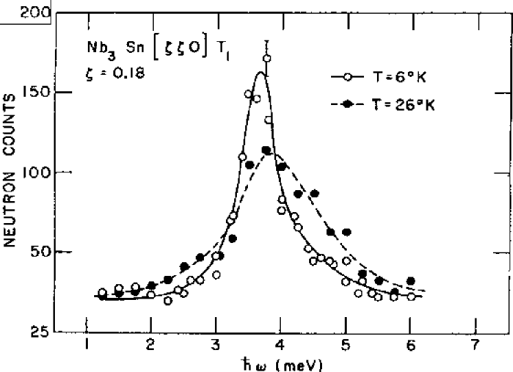
Figure 39: The widths of low energy $[\zeta\zeta 0]T_{1}$ acoustic phonons broaden appreciably at temperatures above $T_{c}$, the superconducting transition temperature. This figure shows the same phonon profile above and below $T_{c}\approx 18.0\ K$ Reproduced from [305].

The classic experiment of this type was performed using neutron scattering on Nb and Nb₃Sn [305]. The idea is simply that the electron charge susceptibility modifies the phonon spectrum. Within the normal state this modification is hardly noticeable in metals over a temperature range of 300 K or so. However, when the material goes superconducting, the electron density of states is profoundly modified at energy scales of order the gap; this in turn will affect phonons whose energy is on the same scale. In particular, a low energy phonon (energy less than $2\Delta$) that had a finite lifetime because it could decay into an electron-hole pair will be unable to do so in the superconducting state because no states exist at energies below the gap, $\Delta$. Therefore its lifetime will lengthen considerably in the superconducting state, resulting in a narrower lineshape below $T_{c}$. Fig. 39 shows the experimental result from Nb₃Sn [305] where the lineshape has clearly become narrower in the superconducting state. Similarly, if the phonon energy is slightly above $2\Delta$, then, under the right conditions, the linewidth will increase, since the electron density of states increases in this energy regime in the superconducting state.

A detailed theory of these effects was first given in Ref. [306], within BCS theory. The theory consists of a calculation of a response function corresponding to a Case I observable. Similar calculations were performed much later by Zeyher and Zwicknagl [268] to understand the frequency shifts and linewidth changes (due to superconductivity) in the ${\bf q}=0$ Raman spectra for various optical modes in YBaCu₃O_7-x. They found, using the BCS approximation,

$${Re\ \Delta\Pi({\bf q}=0,\nu+i\delta)\over N(0)}=\cases{-{2\over\bar{\nu}\sqrt{1-\bar{\nu}^{2}}}tan^{-1}\Bigl{(}{\bar{\nu}\over\sqrt{1-\bar{\nu}^{2}}}\Bigr{)}&for $\bar{\nu}<1$\cr{1\over\bar{\nu}\sqrt{\bar{\nu}^{2}-1}}ln\Bigl{(}2\bar{\nu}^{2}-1+2\bar{\nu}\sqrt{\bar{\nu}^{2}-1}\Bigr{)}&for $\bar{\nu}>1$.\cr}$$ (156)

The imaginary part is given for all temperatures by:

$${Im\ \Delta\Pi({\bf q}=0,\nu+i\delta)\over N(0)}=-\pi\theta(\bar{\nu}-1){tanh\ \beta\nu/4\over\bar{\nu}\sqrt{\bar{\nu}^{2}-1}},$$ (157)

where $\bar{\nu}=\nu/(2\Delta(T))$. Here, $\Delta\Pi({\bf q},\nu+i\delta)$ is the change in the phonon self energy between the superconducting state and the normal state. A positive (negative) real part means that phonons harden (soften) in the superconducting state, while a positive (negative) imaginary part means that the phonon linewidths narrow (broaden). Thus, phonons below the gap edge ($2\Delta$) soften while those above harden. Also, above the gap edge they broaden while below their linewidth does not change. The broadening above $2\Delta$ can be understood as being due to the enhanced scattering with electrons, since the electron density of states now has a square-root singularity in the energy range of $\Delta$, and the phonon self energy is essentially a convolution of two single electron Green functions (see Eq. (128)).

Eqs. (156,157) have been derived assuming single particle Green functions without impurity scattering. The ${\bf q}=0$ limit is somewhat anomalous in this case, in that the phonon width is already zero in the normal state. Hence, no change can occur in the linewidth in the superconducting state, for frequencies below $2\Delta$. A calculation with impurities [269] provides a non-zero linewidth in the normal state. Because of the gap in the single electron density of states in the superconducting state, this linewidth is reduced to zero when the system enters the superconducting state, so the change in the imaginary part of the phonon self energy is positive. These results are summarized in Fig. 40. Note that the softening below the gap edge is significantly reduced with impurity scattering present, and the phonons above $2\Delta$ also soften when a significant degree of impurity scattering is present. As Fig. 40b shows, phonons whose energy lies below $2\Delta$ acquire a narrower linewidth in the superconducting state, as noted above.

The effects of retardation on the phonon self energy are not very significant. The changes that do occur follow the changes already discussed due to including elastic scattering; high energy phonons soften rather than harden, and the broadening that accompanies this softening is reduced compared to the clean BCS case. More detailed changes are documented in Refs. [268, 269].

Because these phonon changes can be observed through neutron scattering experiments, it is of interest to examine the phonon self energy at non-zero momentum, ${\bf q}$ [270, 271]. In this case the phonon has a non-zero linewidth in the normal state, and so line narrowing is observed in superconducting state at low frequencies, due to the development of a single electron gap. The detailed frequency dependence is a function of the band structure; in particular, with two dimensional nesting phonon changes due to superconductivity are enhanced [271].

7 Summary

We have examined a variety of ways in which the retarded electron phonon interaction influences the properties of a conventional superconductor. The first and simplest effect is through a renormalization of Fermi Liquid parameters, like the effective mass. While this effect appears in a number of normal state properties (for example, the low temperature electronic specific heat capacity, where the Sommerfeld $\gamma$ is enhanced by $1+\lambda$ — see Eq. (120)), it also appears in many superconducting properties. The most obvious (but least measurable) example is in the $T_{c}$ equation, Eq. (92), where $1+\lambda$ appears in the exponent. Another (perhaps more detectable) occurrence is in the slope of the upper critical magnetic field. In each of these cases, the renormalization occurs in the normal state — its occurence in the superconducting state is because the property in question depends on the normal state effective mass, or Fermi velocity, etc. One should also bare in mind that the factor $1+\lambda$, comes from a weak coupling approach. In a strong coupling approach, an electron phonon renormalization is still present, but may be much more significant than suggested by the weak coupling approach, and polaron-like physics may dominate [97].

The most important manifestation of the electron phonon interaction is the superconducting state itself. In fact, according to our present understanding of Cooper pairing, the electron phonon-induced attraction between two electrons would not overcome their direct Coulomb repulsion, except for the fact that the former is retarded whereas the latter is not. This gives rise to the pseudopotential effect; in some sense the pseudopotential effect is the true mechanism of superconductivity, rather than the electron phonon interaction per se. This is perhaps emphasized in the cuprate materials, where presumably the electrons could not utilize the difference in energy (and hence time) scales between the attractive mechanism (whatever it is) and the direct Coulomb repulsion to overcome the latter. Instead the pairing has apparently adopted a different symmetry (d-wave) to avoid the direct Coulomb repulsion.

Nonetheless a minimal accounting for these retardation effects accounts fairly well for the superconducting ground state. This was accomplished by BCS theory. A more accurate theory with retardation effects (Eliashberg theory) quite clearly accounts for quantitative discrepancies with experiment. Here, Pb and Hg are held up as paradigms for retardation effects, the simplest occurring in a measurement of the gap ratio, for example. The BCS theory predicts a universal number for this ratio, $2\Delta/k_{B}T_{c}=3.53$. With Eliashberg theory a value for Pb is found close to 4.5, in excellent agreement with experiment. We have characterized the discrepancy with BCS theory through a retardation parameter, $T_{c}/\omega_{\ln}$. Various properties have been quantitatively accounted for through simple analytical expressions with this parameter, as given in Sections 4 and 5 (see Ref. [11] and references therein for many more).

Finally, various dynamical properties exhibit ‘signatures’ of the electron-phonon pairing. These tend to manifest themselves as ‘wiggles’ in the data, the most famous of which occurs in the tunneling data, and allows an inversion to extract the electron phonon spectral function, $\alpha^{2}F(\nu)$. As we saw briefly in Section 3, and then again in Section 6, these ‘wiggles’ occur in various two-electron response functions, most prominent of which is the optical conductivity. An accurate measurement of these response functions allows one to infer a significant electron-phonon coupling.

We have focussed on very conventional superconductors, and have, for example, avoided any analysis of the high temperature superconductors. Signs of electron phonon interactions have occurred in these new materials as well, but the relation to the superconductivity in them is yet unclear. Moreover, such effects will no doubt be covered in other chapters. Nonetheless, we wish to add a few remarks about other classes of superconducting materials that have been discovered over the last twenty years.

Cubic Perovskites, beginning with strontium titanate (SrTiO₃) [61, 62], have already been discussed in Section 2. As mentioned there, these compounds (including BaPb_0.75Bi_0.25O₃   ($T_{c}\approx 12$ K) [63] and Ba_1-xK_xBiO₃    ($T_{c}\approx 30$ K) [65]) are generally regarded as in a distinct class from the high $T_{c}$ cuprates. This has left them, somewhat by default, as electron-phonon driven superconductors. On the other hand, there is strong optical evidence [294, 186] that the electron phonon interaction is very weak in these materials. Hence, as far as we are concerned, the mechanism of superconductivity in these perovskites is not understood at all. Tunneling studies [297, 298] are divided on this issue.

One- and two-dimensional organic superconductors were discovered in 1979 [307]. The subject had developed sufficiently so that, by 1990, a book devoted to the topic was written [308]. Organic superconductivity represents another interesting idea that was first presented by theorists [106, 107], on the basis of a phonon-mediated interaction, but that now is considered by most practitioners not to be due to electron phonon interactions. Many of the organics abound in physical phenomena, with several containing, on the same phase diagram, charge density wave (CDW) and spin density wave (SDW) instabilities, juxtaposed with superconductivity [309]. The nature of the superconducting state has not really been sharply defined by experiments, to the extent that both singlet and triplet pairing may be present [310], and the presence of a gap has not been unequivocally established. While it is probably fair to say that the electron phonon interaction has not been ruled out as the mechanism for superconductivity, spin fluctuation-mediated pairing seems to be favoured [309].

Heavy Fermion systems were discovered to be superconducting also in 1979 [311]. While $T_{c}$ has remained low, these compounds have remained of interest because (i) the root cause of the heavy electron mass is not completely understood, and (ii) the superconducting ground state coexists in a number of cases with antiferromagnetic order. It has now been established through thermal conductivity measurements that the order parameter contains nodes [312], and the circumstantial evidence points towards an unconventional magnetically mediated mechanism for superconductivity [313]. There is very little indication that superconductivity in this class of compounds has anything to do with the electron-phonon interaction.

Superconductivity in alkali-doped buckminster fullerene (A₃C₆₀, with A = K, Rb, Cs) was briefly mentioned earlier in this chapter. On the basis of optical measurements [314], a sizable electron phonon coupling was inferred, and, in fact $\alpha^{2}F(\nu)$ was extracted by an inversion procedure outlined in Section (3.3.3) [178]. Evidence for electron phonon-mediated superconductivity was also presented in earlier reviews [77]. On the other hand, doubts remain concerning the validity of a weak coupling framework [315]. One would like to understand the ‘bigger picture’, i.e. the progression from insulator with pure C₆₀ through the superconducting phase with A₃C₆₀, and back to insulator with A₆C₆₀. In fact, band structure calculations [316] suggest (simplisticly) that A₂C₆₀ should be superconducting with a higher $T_{c}$ than A₃C₆₀, when, in fact, that compound does not readily form.

The electron phonon theory can be subjected to even more tests, now that workers have managed to fabricate a field effect transistor which allows electron [317] and hole [318] doping of C₆₀. $T_{c}$ is much higher for hole doping ($T_{c}=52$ K), and spans a wide range of dopant concentration. In fact this peculiar asymmetry between electron and hole doping finds a natural explanation through the hole mechanism of superconductivity [319]. An explanation in terms of a dopant-dependent electron phonon coupling strength appears somewhat unnatural.

The borocarbides (RNi₂B₂C, where R denotes a rare earth element) were found to be superconducting in 1993 [320, 321]. In addition to having a sizeable transition temperature ($T_{c}\approx 20$ K), some of these compounds exhibit coexistent superconductivity and antiferromagnetic order, and indeed, share some similarities with the heavy fermion compounds [322]. Nonetheless, tunneling has determined that a well-defined gap exists at low temperatures, and this and other measurements have established these compounds to have very BCS-like properties [323]. A detailed comparison of various superconducting properties with results based on Eliashberg theory (including some small anisotropy) [324] yields excellent agreement. A model spectrum was used for the electron phonon interaction, and, at present, it remains unclear to what extent this agreement points unequivocally to the electron phonon mechanism for superconductivity in these compounds.

Very recently, superconductivity with $T_{c}=39$ K has been discovered in the very simple binary compound, MgB₂ [325]. Preliminary results indicate a gap in the single electron density of states [326, 327, 328], and an isotope effect has been observed [329]. Calculations of the electron phonon coupling strength, not quite consistent with $T_{c}=39$ K, have been reported [330], as has a competing non-electron phonon mechanism, based on the hole mechanism [331]. More experimental results will be required before a real assessment of the electron phonon mechanism can be provided.

Finally, Sulfur has been found to exhibit a high superconducting transition temperature ($T_{c}=17$ K) [332]. Very little work has been carried out regarding the mechanism; a notable exception is Ref. [333], where ab initio calculations are performed to estimate the electron phonon coupling strength for Sulfur. They find that under pressure, in a different structural phase, the electron phonon coupling is enhanced, consistent with the increase in $T_{c}$.

As is evident by the foregoing examples, a steady search for new superconductors is being rewarded with discoveries of materials with high critical temperatures, now in the same category as those of the high temperature cuprates. The A15 compound record of $T_{c}\approx 23$ K would have been broken many times by now, even if the layered cuprates had not been discovered. Most intriguing is the fact that many of these compounds may be driven to the superconducting state through the electron phonon mechanism. As far as future developments in this area is concerned, an obvious question to be addressed is the soundness of the original Cohen-Anderson estimate [194] for the maximum electron phonon mediated critical temperature. It may simply be a matter of quantitative assessment, or perhaps some more exotic effect (within the electron phonon picture) has been overlooked. An intermediate or strong coupling approach [97] may yet provide new insights. Finally, one can’t help but notice the recent resurgence of investigations in the high temperature cuprates themselves, that indicate strong electron phonon effects [334]. To paraphrase [335], ’The fat lady probably hasn’t yet sung’.

8 Appendix: Microscopic Developments

In this Appendix, we will first outline a derivation of Eliashberg theory, based on a weak coupling approach. By this we mean that we start with momentum eigenstates. While other derivations may be given in other chapters, we include one here to keep this chapter somewhat self-contained. Migdal theory follows by simply dropping the anomalous amplitudes in what follows. We will then outline various other attempts to understand electron phonon interactions, particularly in the strong coupling regime.

8.1 Migdal-Eliashberg Theory

We begin with the definition of the one electron Green function, defined in momentum space, as a function of imaginary time [83],

$$G({\bf k},\tau-\tau^{\prime})\equiv-<T_{\tau}c_{{\bf k}\sigma}(\tau)c^{\dagger}_{{\bf k}\sigma}(\tau^{\prime})>,$$ (158)

where ${\bf k}$ is the momentum and $\sigma$ is the spin. The angular brackets denote, as usual, a thermodynamic average. With this definition such a Green function can be Fourier expanded in imaginary frequency:

$$G({\bf k},\tau)={1\over\beta}\sum_{-\infty}^{\infty}e^{-i\omega_{m}\tau}G({\bf k},i\omega_{m})$$

$$G({\bf k},i\omega_{m})=\int_{0}^{\beta}d\tau G({\bf k},\tau)e^{i\omega_{m}\tau}.$$ (159)

The frequencies $i\omega_{m}$ are known as the Matsubara frequencies, and are given by $i\omega_{m}=i\pi T(2m-1)$, $m=0,\pm 1,\pm 2,...$, where $T$ is the temperature. Because the $c$’s are Fermion operators, the Matsubara frequencies are odd multiples of $i\pi T$. As is evident from these equations, the imaginary time $\tau$ takes on values from 0 to $\beta$ ($\equiv{1\over k_{B}T}$).

Similar definitions hold for the phonon Green function:

$$D({\bf q},\tau-\tau^{\prime})\equiv-<T_{\tau}A_{\bf q}(\tau)A_{-{\bf q}}(\tau^{\prime})>,$$ (160)

where $A_{\bf q}(\tau)\equiv a_{\bf q}(\tau)\phantom{a}+\phantom{a}a_{-{\bf q}}^{\dagger}(\tau)$. The Fourier transform is similar to that given in Eq. (159) except that the Matsubara frequencies are $i\nu_{n}\equiv i\pi T2n$, $n=0,\pm 1,\pm 2,...$ i.e. they occur at even multiples of $i\pi T$.

To derive the Eliashberg equations, we use the equation-of-motion method, taken from Ref. [57]. The starting point is the (imaginary) time derivative of eq. (158)

$${\partial\over\partial\tau}G({\bf k},\tau)=-\delta(\tau)\phantom{a}-\phantom{a}<T_{\tau}\bigl{[}H-\mu N,c_{{\bf k}\sigma}(\tau)\bigr{]}c^{\dagger}_{{\bf k}\sigma}(0)>,$$ (161)

where, without loss of generality, we have put $\tau^{\prime}=0$. For definiteness, we use the Hamiltonian (3), and, in addition, assume, for the Coulomb interaction, the simple Hubbard model, $H_{Coul}=U\sum_{i}n_{i\uparrow}n_{i\downarrow}$. The sum result is

$$H=\sum_{{\bf k}\sigma}\epsilon_{\bf k}c^{\dagger}_{{\bf k}\sigma}c_{{\bf k}\sigma}+\sum_{\bf q}\hbar\omega_{\bf q}a^{\dagger}_{\bf q}a_{\bf q}+{1\over\sqrt{N}}\sum_{{\bf k}{\bf k}^{\prime}\atop\sigma}g({\bf k},{\bf k}^{\prime})\bigl{(}a_{{\bf k}-{\bf k}^{\prime}}+a^{\dagger}_{-({\bf k}-{\bf k}^{\prime})}\bigr{)}c^{\dagger}_{{\bf k}^{\prime}\sigma}c_{{\bf k}\sigma}\,\,+\,\,{U\over N}\sum_{\bf k,k^{\prime},q}c^{\dagger}_{{\bf k}\uparrow}c^{\dagger}_{{\bf-k+q}\downarrow}c_{{\bf-k^{\prime}+q}\downarrow}c_{{\bf k^{\prime}}\uparrow},$$ (162)

where the various symbols have already been defined in the text. Working out the commutator on Eq. (161) is then straightforward. We obtain

$$\Biggl{(}{\partial\over\partial\tau}+\epsilon_{{\bf k}}\Biggr{)}G_{\uparrow}({\bf k},\tau) = -\delta(\tau)-{1\over\sqrt{N}}\sum_{{\bf k}^{\prime}}g_{{\bf k}{\bf k}^{\prime}}<T_{\tau}A_{{\bf k}-{\bf k}^{\prime}}(\tau)c_{{\bf k}^{\prime}\uparrow}(\tau)c^{\dagger}_{{\bf k}\uparrow}(0)>$$ (163)

$$+{U\over N}\sum_{\bf pp^{\prime}}<T_{\tau}c_{{\bf p^{\prime}-k+p}\downarrow}^{\dagger}(\tau)c_{{\bf p^{\prime}}\downarrow}(\tau)c_{{\bf p}\uparrow}(\tau)c^{\dagger}_{{\bf k}\uparrow}(0)>,$$

where for definiteness we are considering the Green function with $\sigma=\uparrow$. On the right-hand side of Eq. (163) various higher order propagators appear; to determine them an equation of motion would have to be written, which would, in turn, generate even higher order propagators, eventually leading to a set of equations with hierarchical structure. This infinite series is normally truncated at some point by the process of decoupling, which is simply an approximation procedure. For example, in Eq. (163) the Coulomb term is normally not expanded further; instead a decoupling procedure is employed. Thus, under normal circumstances, the last term would become

$$<T_{\tau}c_{{\bf p^{\prime}-k+p}\downarrow}^{\dagger}(\tau)c_{{\bf p^{\prime}}\downarrow}(\tau)c_{{\bf p}\uparrow}(\tau)c^{\dagger}_{{\bf k}\uparrow}(0)> \rightarrow <T_{\tau}c_{{\bf p^{\prime}-k+p}\downarrow}^{\dagger}(\tau)c_{{\bf p^{\prime}}\downarrow}(\tau)><T_{\tau}c_{{\bf p}\uparrow}(\tau)c^{\dagger}_{{\bf k}\uparrow}(0)>,$$ (164)

$$\rightarrow -\delta_{{\bf k}{\bf p}}G_{\downarrow}({\bf p^{\prime}},0)G_{\uparrow}({\bf k},\tau).$$

The case of the electron-phonon term is a little more subtle, however. In this case we define a Green function,

$$G_{2}({\bf k},{\bf k}^{\prime},\tau,\tau_{1})\equiv<T_{\tau}A_{{\bf k}-{\bf k}^{\prime}}(\tau)c_{{\bf k}^{\prime}\uparrow}(\tau_{1})c^{\dagger}_{{\bf k}\uparrow}(0)>,$$ (165)

and write out an equation of motion for it. We get

$${\partial\over\partial\tau}G_{2}({\bf k},{\bf k}^{\prime},\tau,\tau_{1})=-\omega_{{\bf k}-{\bf k}^{\prime}}<T_{\tau}P_{{\bf k}-{\bf k}^{\prime}}(\tau)c_{{\bf k}^{\prime}\uparrow}(\tau_{1})c^{\dagger}_{{\bf k}\uparrow}(0)>,$$ (166)

where $P_{\bf q}(\tau)=a_{\bf q}(\tau)-a_{-{\bf q}}(\tau)$. Taking another derivative yields

$$\Biggl{[}{\partial^{2}\over\partial\tau^{2}}-\omega_{{\bf k}-{\bf k}^{\prime}}\Biggr{]}G_{2}({\bf k},{\bf k}^{\prime},\tau,\tau_{1})=\sum_{{\bf k}^{\prime\prime}\sigma}2\omega_{{\bf k}-{\bf k}^{\prime}}g_{{\bf k}-{\bf k}^{\prime}}<T_{\tau}c^{\dagger}_{{\bf k}^{\prime\prime}-{\bf k}+{\bf k}^{\prime}\sigma}(\tau)c_{{\bf k}^{\prime\prime}\sigma}(\tau)c_{{\bf k}^{\prime}\uparrow}(\tau_{1})c^{\dagger}_{{\bf k}\uparrow}(0)>.$$ (167)

One might be tempted to decouple Eq. (167) and thus close the hierarchy that begins with Eq. (163). However, retardation effects are properly included only when the phonon propagator is taken into account. While the electron-phonon interaction affects the phonons as well as the electrons, the influence on the phonons occurs most at higher temperatures. For many materials the phonons have reached their ground state configurations by about room temperature. As a result, for low temperatures the phonons remain virtually unaffected by the electron-phonon interaction, and it suffices to disregard the electron-phonon interaction as far as the phonons are concerned provided they have been properly renormalized due to effects which took place at higher temperature. To put this another way, inelastic neutron scattering measurements of the phonon dispersion curves show a dependence on temperature only at temperatures well above room temperature [89, 90].

As already mentioned in the text, the phonons are normally taken from experiment, and hence the “calculation” of the phonon propagator is greatly simplified. One simply assumes that the phonons are non-interacting. The equation of motion for the phonon propagator is then

$$\Biggl{(}{\partial^{2}\over\partial\tau^{2}}-\omega_{\bf q}^{2}\Biggr{)}D({\bf q},\tau-\tau^{\prime})=2\omega_{\bf q}\delta(\tau-\tau^{\prime}).$$ (168)

Utilizing this expression in eq. (167) then yields

$$G_{2}({\bf k},{\bf k}^{\prime},\tau,\tau)={1\over N}\sum_{{\bf k}^{\prime\prime}\sigma}\int_{0}^{\beta}d\tau^{\prime}g_{{\bf k}{\bf k}^{\prime}}D({\bf k}-{\bf k}^{\prime},\tau-\tau^{\prime})<T_{\tau}c^{\dagger}_{{\bf k}^{\prime\prime}-{\bf k}+{\bf k}^{\prime}\sigma}(\tau^{\prime})c_{{\bf k}^{\prime\prime}\sigma}(\tau^{\prime})c_{{\bf k}^{\prime}\uparrow}(\tau)c^{\dagger}_{{\bf k}\uparrow}(0)>,$$ (169)

where now $\tau_{1}$ has been set equal to $\tau$ as is required in Eq. (163). This can now be substituted into Eq. (163), and the whole result can be Fourier transformed (from imaginary time to imaginary frequency). Before stating the result of this exercise, however, we note that the superconducting state is specially characterized by the existence of anomalous amplitudes, attributed to Gorkov [44] and often referred to as Gorkov amplitudes. Thus, in the Wick decomposition [83] of the various two-particle Green functions, the anomalous amplitudes also must be taken into account, in addition to the normal amplitudes given, for example, in Eq. (164).

The anomalous amplitudes take the form

$$F({\bf k},\tau)\equiv-<T_{\tau}c_{{\bf k}\uparrow}(\tau)c_{-{\bf k}\downarrow}(0)>$$ (170)

and

$$\bar{F}({\bf k},\tau)\equiv-<T_{\tau}c^{\dagger}_{-{\bf k}\downarrow}(\tau)c^{\dagger}_{{\bf k}\uparrow}(0)>.$$ (171)

Now it is necessary to go through the same procedure with $F$ and $\bar{F}$ as with $G$. The methodology is the same, so we skip the necessary steps.

We then define two self-energies, the usual one (generalized to the superconducting state), denoted by $\Sigma({\bf k},i\omega_{m})$, and an anomalous self-energy, often called the pairing function, $\phi({\bf k},i\omega_{m})$, and we arrive at Eqs.(42-46).

8.2 The Polaron Problem

A rather different and less developed approach to the electron phonon problem focuses on the effect of the phonons on a single electron. A review is provided in Ref. [97], and we merely highlight some of the important points here.

There are many kinds of polarons, i.e. small vs. large, weakly coupled vs. strongly coupled, Fröhlich vs. Holstein, etc. As far as we can tell these classifications are merely qualitative, so that, in most cases, distinctions can be readily drawn for extreme parameters only. A case in point is the distinction between an itinerant vs. self-trapped polaron. It seems clear that no such transition exists, but nonetheless a crossover occurs to a regime in which the polaron acquires a very large effective mass.

In thinking about the polaron problem, there is the usual competition between kinetic energy (measured by the hopping integral, $t$, or the bandwidth, $D=2zt$, where $z$ is the coordination number for a cubic lattice ($z=2,4$ and $6$ in 1,2, and 3 dimensions, respectively)) and the potential energy (measured by $g$ — see Hamiltonian (5)). In addition the phonon frequency represents a third energy scale. In the case of the Holstein model, Eq. (5), this scale is conveniently represented by a single number, the Einstein oscillator frequency, $\omega_{E}$. A dimensionless coupling constant, $\lambda\equiv 2g^{2}/(D\omega_{E})$, corresponds roughly to the enhancement parameter introduced in section 2.3 (see Eq. (21)). Note that in terms of the parameters of the original Holstein Hamiltonian, Eq. (4), $\lambda\equiv\alpha^{2}/(KD)$. An increase in $\lambda$ signifies an approach to the strong coupling limit. On the other hand the adiabatic (anti-adiabatic) limit is represented by $\omega_{E}/t\rightarrow 0(\infty)$. The values of both ratios strongly influence the number of phonons present. An early review that clearly delineates these different regimes is provided by Ref. [336].

There have been many approaches to solving the polaron problem (as governed by a Hamiltonian like Eq. (4)). Some of the early techniques are amply covered in Ref. [54]; these are exemplified by weak and strong coupling perturbation theory, and variational methods. A review of the perturbation approaches is given in Appendix B and C of Ref. [337]. Weak coupling follows the Migdal approach, while strong coupling utilizes the celebrated Lang-Firsov transformation.

This transformation immediately results in a narrow band, with effective hopping parameter, $t_{\rm eff}=t\exp{(-g^{2}/\omega^{2})}$, along with exponential increases in effective mass and, in the adiabatic regime, number of phonons in the ground state [336, 338].

With the advent of considerable computing capabilities over the last two decades, exact methods have been used, that, in various cases, can span the entire parameter regime. The first is Monte Carlo for a single electron, pioneered in Ref. [339]. Trugman et al. [340, 341, 161] utilized exact diagonalizations based on a variational Hilbert space obtained from repeated applications of the Hamiltonian on a trial state vector; their most recent results are capable of achieving very high precision. In the meantime, Proetto and Falicov [342] and Ranninger and Thibblin [343] used a truncated Hilbert space for a two-site problem, and performed a straightforward numerical diagonalization. This was followed by work on larger (one-dimensional) lattices (for one electron) in Refs. [344, 345, 337]. Most of this work was performed for a specific model — the Holstein model of electron phonon coupling, already referred to in the text. Further work was carried out also for the BLF (SSH) model, in Ref. [346]. Yet another technique utilizes the density-matrix renormalization group (DMRG) [348] method [349], which has also been extended to many electrons [350]. Another variational technique known as the Global-Local variational method [347] also provides very accurate results for the polaron problem. Finally, two new Monte Carlo methods [352, 353] appear to be particularly powerful in obtaining polaron properties.

In all cases a clearer understanding is emerging; there is no self-trapping transition, in any dimension, although there is a farily abrupt (but still smooth) crossover from weak coupling-like to strong coupling-like. This crossover has now been investigated in 1,2, and 3 dimensions as well as with dynamical mean-field theory, which is exact in infinite dimensions [351].

An actual transition can be observed in higher dimensions in the adiabatic limit ($\omega_{E}=0$) [354]. However, this limit is regarded as somewhat pathological, and not representative of the general case [347].

Finally, some work has been performed on the bipolaron problem, i.e. whether two polarons bind or not. Much of this work is summarized in Ref. [97]. Various discussions of the supporting evidence and difficulties of these theories can be found in Refs. [355, 356, 357]. A related problem has been asked and partially answered in Refs. [337, 358, 161], which is: to what extent will two electrons interacting through phonon exchange and Coulomb repulsion form a Cooper pair, particularly as the stength of the Coulomb repulsion is increased well in excess of the effective strength of the attractive phonon-induced interaction ? In other words, to what degree does the pseudopotential effect play a role in pairing ?

In Ref. [337] one of us found that pairing persists even when the Coulomb interaction strength exceeds that of the electron phonon attraction, and in Ref. [161] this statement was made more precise (see also Ref. [359]). In particular, binding persists only up to a point; for sufficiently large Coulomb repulsion, the pair is no longer bound. While more work is required, this finding implies that the usual pseudopotential reduction, given by Eq. (75), may be too strong. Eq. (75), for example, achieves a large reduction in the limit $\mu(E_{F})\rightarrow\infty$, whereas the result of Ref. [161] says that for two electrons, at least, the binding is lost in this limit.

8.3 Many Electrons on a Lattice

The problem of many interacting electrons is, in many ways, significantly more difficult than that of one or two electrons. The dimension of the Hilbert space grows exponentially, so that exact diagonalizations become prohibitive. A review of methods and results can be found in Ref. [360]. As far as the electron phonon problem is concerned, there is some limited work which utilizes direct diagonalization, usually in the context of the t-J model [361, 362]. Mainly, however, this problem has been approached through Monte Carlo methods, and a variety of (somewhat uncontrolled) Green function techniques.

Monte Carlo methods have an illustrious history [363]. While they are not formally exact (because, for example, of a Trotter [364] breakup), the error introduced by such a decomposition can be controlled. Hence, in principle, and even in practice through extrapolations, one can obtain results which are exact to within some known error.

Some of the first papers to utilize Monte Carlo methods in many body fermion problems (in the condensed matter context) addressed the electron phonon problem [365, 366, 367]. This particular methodology integrated out the fermion degrees of freedom analytically, leaving the boson degrees of freedom to which Monte Carlo algorithms were applied. Various modifications immediately arose, and were used to address the same electron phonon problem [368, 369, 370, 371] as well as electron-electron problems [372]. Much of this work is reviewed in Ref. [68]; a more comprehensive review of the many variants of the Monte Carlo method (in condensed matter) is provided in Ref. [69].

Studies in two dimensions became more feasible in the late 1980’s; an immediate question that was addressed was the competition between superconductivity and the charge density wave (CDW) instability [94, 373, 95]. At half-filling (where simulations are easiest) the CDW instability overwhelms the tendency towards superconductivity, in part because the tight-binding model with nearest neighbour hopping exhibits nesting at half-filling. Vekić et al. [374] explored the impact of next nearest neighbour hopping (to remove the nesting) but found it was difficult to discern whether an incommensurate CDW instability or superconductivity dominates.

Another means of eliminating the CDW is through doping; again most of the work is inconclusive. A third means is through the use of a Hubbard $U$. A study [375] of the so-called Hubbard-Holstein model in two dimensions found that both the CDW and the superconductivity susceptibilities are suppressed as $U$ grows. To our knowledge, however, the pseudopotential effect (where the $U$ would essentially cancel the electron phonon interaction as far as the CDW was concerned, but not as far as superconductivity was concerned) has never been detected in many-electron Monte Carlo studies.

One of the reasons for exact studies of these lattice models (on small lattices) is for use as a benchmark to which diagrammatic methods can be compared. Thus, for example, the conclusion in Ref. [95] was that the Migdal formalism, without vertex corrections, described the Monte Carlo results fairly accurately, provided phonon renormalization was taken into account. A model system is required to determine this, since, in real systems, the phonons are often taken from experiment, and already contain renormalization effects. This conclusion was confirmed in Ref. [375], as well as in Ref. [376]. In this latter reference, the authors developed the formalism even further to accommodate a CDW gap, and found good agreement with Monte Carlo results.

Nonetheless, it is probably safe to say that a reliable formalism has not yet been developed to investigate low temperature properties of electron phonon systems, particularly slightly away from half-filling. A number of attempts have been made, particularly in the case of electron-electron interactions [377, 378], although a comprehensive treatment has not yet been achieved (the many-body approaches are also becoming almost as numerically intensive as the Monte Carlo methods, and so one of their advantages is diminishing).

Attempts have also been made to incorporate specific kinds of corrections to the Migdal-Eliashberg formalism. One of these categories is the inclusion of vertex corrections. Many feel that they may be necessary because the adiabatic ratio $\omega_{D}/E_{F}$ is not small in some cases (eg. high $T_{c}$ cuprates, and doped buckyballs). In the cuprate materials two-dimensional effects may enhance vertex corrections as well. Calculations showing an enhancement of $T_{c}$ due to vertex corrections have been reported in Ref. [379] (for a two-dimensional gas). In Ref. [380], a different tack is taken; $T_{c}$ is kept fixed, and calculations with vertex corrections included can mimic those without through an adjusted $\mu^{\ast}$ (except for the isotope effect). In Ref. [381] a two-dimensional tight-binding model is used and once again, the conclusion is that vertex corrections enhance the pairing interaction. To our knowledge, however, these effects have never been observed in exact or controlled calculations.

Figure 3: Real and Imaginary parts of the electron self energy in the normal state, for an Einstein spectrum ($\lambda=1$). The dotted lines are the inverse non-interacting electron Green functions, $\omega-(\epsilon_{\bf k}-\mu)$, for $(\epsilon_{\bf k}-\mu)/\omega_{E}=-4,0$, and $4$, from top to bottom, respectively.

Figure 4: The spectral function for an electron interacting with phonons (Einstein spectrum with $\lambda=1$) for various momenta as labelled. Note that for each momentum there is a delta function contribution (artificially broadened in this figure) whose weight diminishes as one moves away from the chemical potential and whose frequency approaches the Einstein phonon frequency. The incoherent component grows with increasing $\epsilon_{\bf k}-\mu$, and approaches a reasonably well-defined peak centered around $\epsilon_{\bf k}-\mu$ for large values (eg. dot-dashed curve).

Figure 10: The electron-phonon spectral function $\alpha^{2}F(\omega)$ (solid curve) for $Pb_{.40}T\ell_{.60}$ determined from tunneling experiments and convoluted by instrument resolution of the neutron spectrometer compared with the neutron results for the phonon frequency distribution $F(\omega)$ (dashed curve) measured by incoherent inelastic neutron scattering [145] (upper frame). The lower frame shows the tunneling results (solid curve) compared with the phonon frequency distribution (dashed curve) determined from a Born von Karman analysis of the phonon dispersion curves in $Pb_{.40}T\ell_{.60}$ [144].

Figure 18: The universal function $G(\bar{\Omega})$ as a function of normalized phonon energy $\bar{\Omega}=\Omega/T_{c}$ which enters the curve for the functional derivative of $T_{c}$ with respect to $\alpha^{2}F(\omega)$ in the $\lambda^{\Theta\Theta}$ model of Ref. [195], from which this figure was taken.

Figure 19: The constant $c(\mu^{*})$ in the relation $k_{B}T_{c}=c(\mu^{*})A$ for the maximum $T_{c}$ associated with a given A as a function of $\mu^{*}$. Placed on the same figure (solid dots) are the results for $T_{c}/A$ obtained in the case of many strong coupling superconductors for which $\alpha^{2}F(\omega)$ is known from tunneling spectroscopy. The solid points all fall below the maximum curve as they must. Adapted from Ref. [196].

Figure 20: The isotope coefficient, $\beta$, vs. $T_{c}$, for various values of $\lambda$ and $\omega_{E}$. Along each curve $T_{c}$ changes because the Coulomb pseudopotential $\mu^{\ast}$ is being varied. These results show that a low value of $\beta$ is difficult to attain with high $T_{c}$. On the other hand, for low $T_{c}$ materials, it is not so difficult.

Figure 21: (a) The temperature dependence of the BCS order parameter, and (b) the resulting densities of states at various temperatures below $T_{c}$. The only effect of finite temperatures on these latter curves is a reduced gap.

Figure 22: (a) $\Delta(i\omega_{n})$ and $Z(i\omega_{n})$ vs $\omega_{n}$, the fermion Matsubara frequency, for various temperatures, as indicated. Note that the curves are relatively smooth and featureless, and at low temperatures little change occurs, except that more Matsubara frequencies are present. In (a) the units of $\Delta$ are meV. These were produced for Pb.

Figure 23: The (a) real and (b) imaginary parts of the gap function (in meV) on the real frequency axis, for Pb, for various temperatures, as in the previous figure. Note the considerable structure present on the real axis. Also shown is the (c) real and (d) imaginary part of the renormalization function, $Z(\omega)$ vs $\omega$.

Figure 24: Calculated densities of states of Pb for various temperatures. In contrast to the BCS case (Fig. (21b), at high temperatures there is considerable smearing.

Figure 26: Specific heat of aluminium as a function of temperature in the superconducting state and the normal state (applied field of 300 Gauss). Data taken from Ref. [235]. The BCS prediction, given the normal state data, is given by the solid curve.

Figure 27: The specific heat ratio, $\Delta C(T_{c})/(\gamma T_{c})$ vs $T_{c}/\omega_{\ell n}$. The dots represent results from the full numerical solutions of the Eliashberg equations. Experiment tends to agree to within 10%. In increasing order of $T_{c}/\omega_{\ell n}$, the dots correspond to the following systems: $A\ell$, $V$, Ta, Sn, $T\ell$, $T\ell_{0.9}Bi_{0.1}$, In, Nb (Butler), Nb (Arnold), $V_{3}Si\ 1$, $V_{3}Si$ (Kihl.), Nb (Rowell), Mo, $Pb_{0.4}T\ell_{0.6}$, La, $V_{3}Ga$, $Nb_{3}A\ell(2)$, $Nb_{3}Ge(2)$, $Pb_{0.6}T\ell_{0.4}$, Pb, $Nb_{3}A\ell(3)$, $Pb_{0.8}T\ell_{0.2}$, Hg, $Nb_{3}Sn$, $Pb_{0.9}Bi_{0.1}$, $Nb_{3}A\ell(1)$, $Nb_{3}Ge(1)$, $Pb_{0.8}Bi_{0.2}$, $Pb_{0.7}Bi_{0.3}$, and $Pb_{0.65}Bi_{0.35}$. The drawn curve corresponds to $\Delta C(T_{c})/\gamma T_{c}=1.43(1+53(T_{c}/\omega_{\ell n})^{2}\ell n(\omega_{\ell n}/3T_{c}))$. Adapted from Ref. [221].

Figure 28: (a) $\sigma_{1}(\nu)$ vs. $\nu$ in the zero temperature BCS superconducting state for the various impurity scattering rates indicated. The absorption onset at $2\Delta(0)$ remains sharp independent of the scattering rate. A delta-function contribution (not shown) is also present at the origin. (b) Same as in (a) except for the frequency times the imaginary part of the conductivity. The optical gap is a little less evident in the dirty limit. The conductivity is given in units of $ne^{2}/m\equiv\omega_{P}^{2}/4\pi$). Taken from Ref. [181].

Figure 29: Frequency dependence of $\sigma_{1}(\nu)$ near the clean limit ($1/\tau=1$ meV) for various temperatures in the BCS superconducting state. The appearance of a gap is evident, even at temperatures close to $T_{c}$. (b) Same as in (a), but for $\nu\sigma_{2}(\nu)$. The appearance of a gap is evident in the imaginary part of the conductivity as well. The conductivity is given in units of $ne^{2}/m\equiv\omega_{P}^{2}/4\pi$). Taken from Ref. [181].

Figure 30: Frequency dependence of $\sigma_{1}(\nu)$ near the dirty limit ($1/\tau=25$ meV) for various temperatures in the BCS superconducting state. The appearance of a gap is evident, even at temperatures close to $T_{c}$. (b) Same as in (a), but for $\nu\sigma_{2}(\nu)$. The appearance of a gap is evident in the imaginary part of the conductivity as well. The conductivity is given in units of $ne^{2}/m\equiv\omega_{P}^{2}/4\pi$).

Figure 31: Nuclear spin relaxation rate vs. reduced temperature. Data points for Indium are indicated by circles and triangles, while data for YBa₂Cu₃O₇ are indicated by squares and crosses. The solid curves are calculated with Eliashberg theory for Indium (upper curve) and two model spectra with $\lambda=1.66$ and $3.2$ (lowest curve). Agreement is good in the case of Indium and the lowest curve. Reproduced from [168].

Figure 32: (a) Conductivity ratio, $\sigma_{1s}/\sigma_{1n}$, versus reduced temperature, $T/T_{c}$, in the BCS limit, for various impurity scattering rates. From top to bottom the curves are calculated for ${1\over\tau\Delta_{0}}=100,2,1,0.5,0.1,0.05$, and $0$. The frequency used was $\nu/\Delta_{0}=0.02.$ In the clean limit $(1/\tau=0)$ the coherence peak has disappeared. (b) Same quantity as in (a), but for different coupling strengths, $\lambda=0.77,1.5,2.3$, and $3.1$. (The peak diminishes with increasing coupling strength). These were computed in the dirty limit $(1/\tau=500$ meV) and for $\nu=0.05$ meV. The result for $\lambda=0.77$ (largest maximum) is nearly identical with the BCS result. (c) Conductivity ratio versus frequency normalized to the zero temperature gap edge, $\nu/\Delta_{0}$, for the same coupling strengths as in (b). The curves decrease in magnitude with increasing coupling strength. The maximum apparent in (b) for $\lambda=0.77$ and $1.5$ is also clear here since the two uppermost curves have magnitude greater than unity. As the coupling strength increases the conductivity ratio becomes independent of frequency. Calculations are in the dirty limit, with $T/T_{c}=0.85$.

Figure 33: Microwave conductivity normalized to the normal state, $\sigma_{1s}/\sigma_{1n}$, as a function of reduced temperature $T/T_{c}$. The open squares are the data for Nb. The dotted curve is the BCS result with experimental frequency $\omega=17$ GHz and impurity scattering rate $1/\tau=100.0$ meV (dirty limit). The solid and dashed curves are the results of full Eliashberg calculations with two different $(\alpha^{2}F(\omega))$ spectra. None of the theoretical curves can reproduce the data.

Figure 34: The real part (a,b) and the imaginary part (c,d) of the conductivity at essentially zero temperature ($T/T_{c}=0.3$) with $1/\tau=2$ meV (a,c) and $1/\tau=25$ meV (b,d). In all cases we have used the BKBO spectrum scaled to give the designated value of, $\lambda$, while $T_{c}$ is held fixed at 29 K by adjusting $\mu^{\ast}$. Increased coupling strength suppresses both $\sigma_{1}(\nu)$ and $\nu\sigma_{2}(\nu)$ and broadens the minimum in the latter at $2\Delta$. Note that $2\Delta$ increases slightly as the coupling strength is increased. The conductivity is given in units of $ne^{2}/m\equiv\omega_{P}^{2}/4\pi$).

Figure 35: Measured $\nu\sigma_{2}(\nu)$ vs. frequency at $T=9$ K and at $T=300$ K (solid curves). Also shown are the theoretical fits, using the BKBO spectrum, scaled so that $\lambda=0.2$ (dashed curves). $T_{c}$ is kept fixed to the experimental value with a negative $\mu^{\ast}$. Finally, theoretical fits are also shown with $\lambda=1$ (dotted curves). The latter curves are clearly incompatible with the experimental results. Adapted from Ref. [186].

Figure 36: The conductivity-derived scattering rate, $1/\tau(\nu)\equiv{\omega_{P}^{2}\over 4\pi}Re\ \bigl{(}1/\sigma(\nu)\bigr{)}$ vs. frequency in the normal state for pure elastic scattering (dashed line), combined elastic and inelastic scattering (BKBO spectrum with $\lambda=1$), and pure inelastic scattering using a model spin fluctuation spectrum appropriate to YBCO. Because of the difference in spectral function frequency scales, the result for YBCO continues to rise with frequency, even at 300 meV. Reproduced from [181].

Figure 37: Conductivity-derived scattering rate, $1/\tau(\nu)$ vs. frequency in the BCS s-wave superconducting state for (a) $1/\tau=2$ meV and (b) $1/\tau=25$ meV. An abrupt onset of absorption at the optical gap at temperatures near $T_{c}$ is more apparent in (a) than in (b). The horizontal dashed line indicates the normal state result. Reproduced from [181].

Figure 38: The conductivity-derived scattering rate, $1/\tau(\nu)$ vs. frequency in the s-wave superconducting state for (a) $1/\tau=0$ meV and (b) $1/\tau=25$ meV, for temperatures as indicated. In both cases we used the BKBO spectrum with $\lambda=1$. In (a) there is no signature for a gap, while one remains at low temperatures in (b).

Figure 40: (a) Real and (b) Imaginary part of $\Delta\Pi(\nu+i\delta)/N(0)$ vs $\nu/(2\Delta_{0})$ at zero temperature, for various impurity scattering rates, $1/(\tau\Delta_{0})=0$ (solid), 1 (dotted), and 6 (dashed), in the weak coupling (BCS) approximation. Below twice the gap edge the phonons soften; above twice the gap edge they harden in the clean limit and soften in the dirty limit. Note the narrowing that occurs below the gap edge in the presence of impurity scattering.

References

- [1] G.M. Eliashberg, Zh. Eksperim. i Teor. Fiz. 38 966 (1960); Soviet Phys. JETP 11 696 (1960).
- [2] Y. Nambu, Phys. Rev. 117 648 (1960).
- [3] P. Morel and P.W. Anderson, Phys. Rev. 125 1263 (1962).
- [4] J.R. Schrieffer, D.J. Scalapino and J.W. Wilkins, Phys. Rev. Lett. 10 336 (1963).
- [5] J. Bardeen, L.N. Cooper and J.R. Schrieffer, Phys. Rev. 106, 162 (1957); Phys. Rev. 108, 1175 (1957).
- [6] B.T. Matthias, in Superconductivity, edited by P.R. Wallace (Gordon and Breach, New York, 1969) p. 225. There is also on record an interesting exchange of theoretical and experimental ideas by P.W. Anderson and B.T. Matthias, in Science 144 373 (1964).
- [7] Note, however, that Bednorz and Müller [8, 9] were motivated by BCS theory and various ideas that would lead to a stronger electron-phonon coupling in metallic oxides.
- [8] J.G. Bednorz and K.A. Müller, Z. Phys. B64, 189 (1986).
- [9] J.G. Bednorz and K.A. Müller, Rev. Mod. Phys. 60 585 (1988).
- [10] P.W. Anderson and C.C. Yu, Proceedings of the International School of Physics “Enrico Fermi”, ed. F. Bassani, F. Fumi, and M. Tosi (North-Holland, Amsterdam, 1983).
- [11] J.P. Carbotte, Rev. Mod. Phys. 62 1027 (1990).
- [12] D. Rainer, in Progress in Low Temperature Physics, Vol. 10, edited by D.F. Brewer (North-Holland, 1986), p.371.
- [13] P.B. Allen and B. Mitrović, in Solid State Physics, edited by H. Ehrenreich, F. Seitz, and D. Turnbull (Academic, New York, 1982) Vol. 37, p.1.
- [14] D.J. Scalapino, in Superconductivity, edited by R.D. Parks (Marcel Dekker, Inc., New York, 1969)p. 449.
- [15] Per Fridtjof Dahl, Superconductivity, Its Historical Roots and Development from Mercury to the Ceramic Oxides (AIP, New York, 1992).
- [16] H.K. Onnes, Comm. Leiden 120b (1911).
- [17] W. Meissner and R. Ochsenfeld, Naturwiss. 21 787 (1933).
- [18] C.J. Gorter, Nature 132 931 (1933).
- [19] See, for example, H. Thomas, in Earlier and Recent Aspects of Superconductivity, edited by J.G. Bednorz and K.A. Müller (Springer-Verlag, New York, 1990) p.31.
- [20] F. London, Superfluids Volume I: Macroscopic Theory of Superconductivity (John Wiley and Sons, New York, 1950).
- [21] Although pairing had actually been proposed several years earlier in a very brief report by Ogg (R.A. Ogg, Jr. Phys. Rev. 69 243 (1946), who thought he had observed superconductivity in Metal-Ammonia solutions at 100 - 200 K.
- [22] An interesting account of the activity at the time is provided by L. Hoddeson, E. Braun, J. Teichmann, and S. Weart, Out of the Crystal Maze (Oxford University Press, New York, 1992).
- [23] E. Maxwell, Phys. Rev. 78 477 (1950).
- [24] C.A. Reynolds, B. Serin, W.H. Wright, and L.B. Nesbitt, Phys. Rev. 78 487 (1950).
- [25] H.K. Onnes and W. Tuyn, Comm. Leiden 160b 451 (1923).
- [26] H. Fröhlich, Phys. Rev. 79 845 (1950).
- [27] J. Bardeen, Phys. Rev. 79 167 (1950).
- [28] H. Fröhlich, Proc. Roy. Soc. A 223 296 (1954).
- [29] L.D. Landau, Phys. Z. Sowjetunion 3 644 (1933).
- [30] H. Fröhlich, Proc. Roy. Soc. A 160 230 (1937).
- [31] H. Fröhlich, H. Pelzer, and S. Zienau, Phil. Mag. 41 221 (1950).
- [32] T.D. Lee and D. Pines, Phys. Rev. 88 960 (1952; T.D. Lee, F.E. Low, and D. Pines, Phys. Rev. 90 297 (1953).
- [33] R.P. Feynman, Phys. Rev. 97 660 (1955).
- [34] T. Holstein, Ann. Phys. 8, 325,343 (1959).
- [35] J. Bardeen and D. Pines Phys. Rev. 99 1140 (1955).
- [36] N.W. Ashcroft and N.D. Mermin Solid State Physics (Saunders College Publishing, New York 1976)p. 518.
- [37] J. Bardeen and J.R. Schrieffer, “Recent Developments in Superconductivity,” in Progress in Low Temp. Physics, ed. C.J. Gorter (New York, Interscience, 1961)p. 170.
- [38] L.N. Cooper, Phys. Rev. 104, 1189 (1956).
- [39] Indeed, the electron-phonon mechanism has been questioned many times over the years since BCS, not just on new superconductors, but on conventional ones as well.
- [40] P.W. Anderson, Phys. Rev. 112, 1900 (1958).
- [41] N.N. Bogoliubov, N.V. Tolmachev, and D.V. Shirkov, A New Method in the Theory of Superconductivity, Consultants Bureau, Inc., New York (1959).
- [42] J. Valatin, Nuovo Cimento, 7, 843 (1958).
- [43] P. G. de Gennes, Superconductivity of Metals and Alloys (W.A. Benjamin, Inc. New York, 1966).
- [44] L.P. Gorkov, Zh. Eksperim. i Teor. Fiz. 34 735 (1958); Sov. Phys. JETP 7 505 (1958).
- [45] V.L. Ginzburg and L.D. Landau, Zh. Eksperim. i. Teor. Fiz. 20 1064 (1950).
- [46] J.R. Schrieffer, Theory of Superconductivity (Benjamin/Cummings, Don Mills, 1964).
- [47] D.J. Scalapino, J.R. Schrieffer and J.W. Wilkins, Phys. Rev. 148 263 (1966).
- [48] I. Giaever, Phys. Rev. Lett. 5 464 (1960).
- [49] J.M. Rowell, P.W. Anderson, and D.E. Thomas, Phys. Rev. Lett. 10 334 (1963).
- [50] W.L. McMillan and J.M. Rowell, Phys. Rev. Lett. 14 108 (1965).
- [51] Superconductivity, edited by R.D. Parks (Marcel Dekker, Inc., New York, 1969).
- [52] W.L. McMillan and J.M. Rowell, in Superconductivity, edited by R.D. Parks (Marcel Dekker, Inc., New York, 1969)p. 561.
- [53] P.W. Anderson, in Superconductivity, edited by R.D. Parks (Marcel Dekker, Inc., New York, 1969)p. 1343.
- [54] Polarons and Excitons edited by C.G. Kuper and G.D. Whitfield (Oliver and Boyd, Edinburgh, 1963).
- [55] There is one sentence in the article by Gladstone et al. G. Gladstone, M.A. Jensen and J.R. Schrieffer, in Superconductivity, edited by R.D. Parks (Marcel Dekker, Inc., New York, 1969)p. 665, (see p. 684), where, however, the polaron concept is simply dismissed from a discussion of metals.
- [56] J.M. Blatt Theory of Superconductivity, (Academic Press, New York, 1964).
- [57] G. Rickayzen, Theory of Superconductivity (John Wiley and Sons, New York, 1965).
- [58] M. Tinkham, Introduction to Superconductivity, (McGraw-Hill, New York, 1975).
- [59] Even in C.G. Kuper, An Introduction to the Theory of Superconductivity (Clarendon Press, Oxford, 1968), there is no reference to the 1963 Scottish Summer School, co-edited by Kuper.
- [60] M.R. Schafroth, Phys. Rev. 96 1442 (1954); 100 463 (1955); J.M. Blatt and S.T. Butler, Phys. Rev. 100 476 (1955); J.M. Blatt, S.T. Butler and M.R. Schafroth, Phys. Rev. 100 481 (1955); S.T. Butler and J.M. Blatt, Phys. Rev. 100 495 (1955); M.R. Schafroth, Phys. Rev. 100 502, (1955).
- [61] M.L. Cohen, Phys. Rev. 134A 511 (1964).
- [62] J.F. Schooley, W.R. Hosler and M.L. Cohen, Phys. Rev. Lett. 12 474 (1964).
- [63] A.W. Sleight, J.L. Gillson and P.E. Bierstedt, Sol. State Commun. 17 27 (1975).
- [64] J.F. Schooley, H.P.R. Frederikse and M.L. Cohen, unpublished, as quoted in M.L. Cohen, in Superconductivity, edited by R.D. Parks (Marcel Dekker, Inc., New York, 1969)p. 615.
- [65] L.F. Mattheiss, E.M. Gyorgy and D.W. Johnson, Jr., Phys. Rev. B37 3745 (1988).
- [66] See, for example, the URL http://large.stanford.edu/rbl/nobel/talk/p2.htm.
- [67] V.I. Anisimov, J. Zaanen, and O.K. Andersen, Phys. Rev. B44 943 (1991).
- [68] D.J. Scalapino, in Frontiers and Borderlines in Many-Particle Physics, edited by R.A. Broglia and J.R. Schrieffer (North-Holland, New York, 1988)p. 364.
- [69] W. von der Linden, Phys. Reports 220 53 (1992).
- [70] S. Barišić, J. Labbé and J. Friedel, Phys. Rev. Lett. 25, 919 (1970).
- [71] W.-P. Su, J.R. Schrieffer, and A.J. Heeger, Phys. Rev. Lett. 42 1698 (1979); Phys. Rev. B22, 2099 (1980).
- [72] H. Fröhlich, in Polarons and Excitons, edited by C.G. Kuper and G.D. Whitfield (Oliver and Boyd, Edinburgh, 1963) p. 1.
- [73] R.P. Feynman, Statistical Mechanics (Addison-Wesley, Don Mills, 1972).
- [74] J. Hubbard, Proc. Roy. Soc. London, Ser. A, 276, 238 (1963); 277, 237 (1964); 281, 401 (1964).
- [75] A.J. Heeger, S. Kivelson, J.R. Schrieffer, and W.-P. Su, Rev. Mod. Phys. 60 781 (1988).
- [76] H. Krakauer, W.E. Pickett and R.E. Cohen, Phys. Rev. B47, 1002 (1993).
- [77] O. Gunnarsson, Rev. Mod. Phys. 69, 575 (1997).
- [78] L.P. Kadanoff and G. Baym, Quantum Statistical Mechanics (W.A. Benjamin, Inc., New York, 1962).
- [79] A.A. Abrikosov, L.P. Gorkov and I.E. Dzyaloshinski, Methods of Quantum Field Theory in Statistical Physics (Dover Publications, Inc. New York, 1963).
- [80] R.D. Mattuck, A Guide to Feynman Diagrams in the Many-Body Problem (Dover Publications, New York, 1976).
- [81] A.L. Fetter and J.D. Walecka, Quantum Theory of Many-Particle Systems (McGraw-Hill Book Company, Toronto, 1971).
- [82] G. Rickayzen, Green’s Functions and Condensed Matter (Academic Press, Toronto, 1980).
- [83] G.D. Mahan. Many-Particle Physics (Plenum Press, New York, 1981).
- [84] A.B. Migdal, Zh. Eksp. Teor. Fiz. 34, 1438 (1958) [Sov. Phys. JETP 7, 996 (1958)].
- [85] S. Englesberg and J.R. Schrieffer, Phys. Rev. 131 993 (1963).
- [86] S. Nakajima, Y. Toyozawa, and R. Abe, The Physics of Elementary Excitations (Springer-Verlag, New York, 1980).
- [87] K. Shimojima and H. Ichimura, Prog. Theor. Phys. 43 925 (1970).
- [88] G. Grimvall, The Electron-Phonon Interaction in Metals (Norht-Holland, New York, 1981).
- [89] B.N. Brockhouse, T. Arase, G. Caglioti, K.R. Rao and A.D.B. Woods, Phys. Rev. 128 1099 (1962).
- [90] R. Stedman, L. Almqvist, G. Nilsson and G. Raunio, Phys. Rev. 162 545, 549 (1967).
- [91] P.B. Allen, Phys. Rev. B13 1416 (1976).
- [92] M. Abramowitz and I.A. Stegun, Handbook of Mathematical Functions (Dover, New York, 1964).
- [93] G. Baym and N.D. Mermin, J. Math. Phys. 2 232 (1961).
-
[94]
R.T. Scalettar, N.E. Bickers and D.J. Scalapino, Phys. Rev. B 40
197 (1989).
R.M. Noack, D.J. Scalapino and R.T. Scalettar, Phys. Rev. Lett. 66 778 (1991).
R.M. Noack and D.J. Scalapino, Phys. Rev. B 47 305 (1993). - [95] F. Marsiglio, Phys. Rev. B 42 2416 (1990); in Electron-Phonon Interaction in Oxide Superconductors, edited by R. Baquero (World Scientific, Singapore, 1991) p.167.
-
[96]
E. Berger, P. Valás̆ek, and W. von der Linden, Phys. Rev. B 52,
4806 (1995).
W. von der Linden, E. Berger and P. Valás̆ek, J. Low Temp. Phys. 99, 517 (1995). - [97] A.S. Alexandrov and N. Mott, Polarons and Bipolarons (World Scientific, Singapore, 1995).
- [98] M. Botti, E. Cappelluti, C. Grimaldi and L. Pietronero, to be published in Int. J. Mod. Phys. B, cond-mat/0007007, July, 2000.
- [99] A.S. Alexandrov, V.N. Grebenev, and E.A. Mazur, Pis’ma Zh. Eksp. Teor. Fiz. 45 357 (1987) [JETP Lett. 45 455 (1987)].
- [100] R.E. Prange and L.P. Kadanoff, Phys. Rev. 134 A 566 (1964).
-
[101]
A.J. Leggett, J. de Physique, C7, 41, 19 (1980);
A.J. Leggett, in Modern Trends in the Theory of Condensed Matter, edited by S. Pekalski and J. Przystawa (Springer, Berlin, 1980)p. 13. - [102] P. Nozières and S. Schmitt-Rink, J. Low Temp. Phys. 59, 195 (1985).
- [103] J.C. Swihart, IBM J. Research Develop. 6 14 (1962); Phys. Rev. 131 73 (1963).
- [104] B.D. Josephson, Phys. Lett. 1 251 (1962).
- [105] See Ref. [13] for more discussion, but note that our notation differs from theirs.
- [106] W.A. Little, Phys. Rev. 134 A1416 (1964).
- [107] V.L. Ginzburg, Zh. Eksp. Teor. Fiz. 47 2318 (1964): Sov. Phys.-JETP 20 1549 (1965).
- [108] N.F. Berk and J.R. Schrieffer, Phys. Rev. Lett. 17 433 (1966).
- [109] M. Grabowski and L.J. Sham, Phys. Rev. B29 6132 (1984).
- [110] Y. Takada, Phys. Rev. B37 155 (1988).
- [111] J.E. Hirsch and D.J. Scalapino, Phys. Rev. B32 117 (1985).
- [112] N.E. Bickers, D.J. Scalapino, and R.T. Scalettar, Int. J. Mod. Phys. B1 687 (1987).
- [113] A. Millis, H. Monien, and D. Pines, Phys. Rev. B 42 167 (1990).
- [114] M. Peter, J. Ashkenazi and M. Dacorogna, Helv. Phys. Acta 50 267 (1977).
- [115] J. M. Daams, PhD Thesis, McMaster (1979).
- [116] J.R. Clem, Ann. Phys. 40 268 (1966).
- [117] H.W. Weber, in Anisotropy Effects in Superconductors (Plenum Press, New York, 1977).
- [118] P. Horsch and H. Rietschel, Z. Phys. B27 153 (1977).
- [119] S.J. Nettel and H. Thomas, Sol. St. Commun. 21 683 (1977).
- [120] S.G. Lie and J.P. Carbotte, Sol. St. Commun. 26 511 (1978).
- [121] P.W. Anderson, J. Phys. Chem. Solids 11 26 (1959).
- [122] P.G. Tomlinson and J.P. Carbotte, Phys. Rev. B13 4738 (1976).
- [123] A.M. Clogston and V. Jaccarino, Phys. Rev. 121 1357 (1961).
- [124] L.R. Testardi, in Physical Acoustics, edited by W.P. Mason and R.N. Thurston (Academic Press, New York, 1973)p. 193.
- [125] M. Weger and I.B. Goldberg, Solid State Physics, edited by M. Ehrenreich, F. Seitz, and D. Turnbull (Academic Press, New York, 1973), Vol. 28, p. 1.
- [126] Yu. A. Izymov and Z.Z. Kurmaev, Usp. Fiz. Nauk. 113 193 (1974); Sov. Phys. Usp. 17 356 (1974).
- [127] B.M. Klein, L.L. Boyer, and D.A. Papaconstantopoulos, Phys. Rev. B18 6411 (1978).
- [128] K.M. Ho, M.L. Cohen, and W.E. Pickett, Phys. Re. Lett. 41 815 (1978).
- [129] W.E. Pickett, in Superconductivity in d- and f- Band Metals, edited by H. Suhl and M.B. Maple (Academic Press, New York, 1980) p. 77.
- [130] B.M. Klein, D.A. Papaconstantopoulos, and L.L. Boyer, in Superconductivity in d- and f- Band Metals, edited by H. Suhl and M.B. Maple (Academic Press, New York, 1980) p. 455.
- [131] M. Gurvitch, A.K. Ghosh, B.L. Gyorrfy, H. Lutz, O.F. Kammerer, J.S. Rosner, and M. Strongin, Phys. Rev. Lett. 41 1616 (1978).
- [132] A.K. Ghosh and M. Strongin, in Superconductivity in d- and f- Band Metals, edited by H. Suhl and M.B. Maple (Academic Press, New York, 1980) p. 305.
- [133] W.E. Pickett, Phys. Rev. B21 3897 (1980).
- [134] B. Mitrović and J.P. Carbotte, Can. J. Phys. 61 758 (1983); 61 784 (1983); 61 872 (1983).
- [135] B. Mitrović, PhD Thesis, McMaster (1981).
- [136] L.Y. Shen, in Superconductivity in d- and f- Band Metals, edited by D.H. Douglass (AIP, New York, 1972) p. 31.
- [137] C.S. Owen and D.J. Scalapino, Physica 55 691 (1971).
- [138] G. Bergmann and D. Rainer, Z. Physik 263 59 (1973).
- [139] D. Rainer and G. Bergmann, J. Low Temp. Phys. 14 501 (1974).
- [140] P.B. Allen and R.C. Dynes, Phys. Rev. B12 905 (1975); see also R.C. Dynes, Solid State Commun. 10 615 (1972).
- [141] J.M. Daams and J.P. Carbotte, J. Low Temp. Phys. 43 263 (1981).
- [142] J.C. Phillips and L. Kleinman, Phys. Rev. 116 287, 880 (1959).
- [143] W.A. Harrison, in Phonons in Perfect Lattices and in Lattices with Point Imperfections, ed. by R.W.H. Stevenson (Oliver and Boyd, Edinburgh, 1966) p.73.
- [144] B.N. Brockhouse, E.D. Hallman and S.C. Ng, in Magnetic and Inelastic Scattering of Neutrons in Metals, edited by T.J. Rowland and P.A. Beck (Gordon and Breach, London, 1968).
- [145] A.P. Roy and B.N. Brockhouse, Can. J. Phys. 48 1781 (1970).
- [146] D. Bohm and T. Staver, Phys. Rev. 84 836 (1950).
- [147] W. Kohn, Phys. Rev. Lett. 2 393 (1959).
- [148] P.G. Tomlinson and J.P. Carbotte, Can. J. Phys. 55 751 (1977).
- [149] M. Appapillai and A.R. Williams, J. Phys. F 3 759 (1973).
- [150] J.R. Anderson and A.V. Gold, Phys. Rev. 139 A1459 (1963).
- [151] B.A. Kotov, N.M. Okuneva, and E.L. Plachenova, Fiz. Tverd. Tela (Leningrad) 10 513 (1968); Sov. Phys. Solid State 10 402 (1968).
- [152] E.R. Cowley, Solid State Commun. 14 587 (1974).
- [153] P.B. Allen, Phys. Rev. 6 2577 (1972).
- [154] P.B. Allen, Solid State Commun. 14 937 (1974).
- [155] H.J. Vidberg and J. Serene, J. Low Temp. Phys. 29, 179 (1977).
- [156] R. Blaschke and R. Blocksdarf, Z. Physik B 49 99 (1982).
- [157] C.R. Leavens and D.S. Ritchie, Solid State Commun. 53 137 (1985).
- [158] F. Marsiglio, M. Schossmann and J.P. Carbotte, Phys. Rev. B37, 4965 (1988).
- [159] N.N. Bogoliubov, N.V. Tolmachev, and D.V. Shirkov, A New Method in the Theory of Superconductivity, (Consultants Bureau, Inc., New York, 1959).
- [160] F. Marsiglio, Physica C 160 305 (1989).
- [161] J. Bonca, T. Katrasnik, and S.A. Trugman, Phys. Rev. Lett. 84 3153 (2000).
- [162] C.R. Leavens and E.W. Fenton, Solid State Commun. 33 597 (1980).
- [163] The reader may notice that this amounts to simply changing the imaginary frequency where it occurs in Eqs. (54,55) to before doing the Matsubara sum.
- [164] R. Meservey and B.B. Schwartz, in Superconductivity, edited by R.D. Parks (Marcel Dekker, Inc., New York, 1969)p. 117.
- [165] C.B. Duke, Tunneling in Solids (Academic, New York, 1969).
- [166] E.L. Wolf, Principles of Electron Tunneling Spectroscopy (Oxford University Press, New York, 1985).
- [167] A.E. Karakozov, E.G. Maksimov and S.A. Mashkov, Zh. Eksp. Teor. Fiz. 68 1937 1975; Sov. Phys.-JETP 41 971 1976.
- [168] P.B. Allen and D. Rainer, Nature 349 396 (1991).
- [169] F. Marsiglio and J.P. Carbotte, Phys. Rev. B43 5355 (1991).
- [170] J.E. Hirsch, private communication.
- [171] E.L. Wolf and J. Zasadzinski, Phys. Lett. A62 165 (1974).
- [172] L.Y. Shen, Phys. Rev. Lett. 29 1082 (1972)
- [173] A.A. Galkin, A.I. D’yachenko, and V.M. Svistunov, Sov. Phys. JETP 39 1115 (1974) [Zh. Eksp. Teor. Fiz. 66 2262 (1974)].
- [174] F. Marsiglio, unpublished.
- [175] R.R. Joyce and P.L. Richards, Phys. Rev. Lett. 24 1007 (1970).
- [176] P.B. Allen, Phys. Rev. B3 305 (1971).
- [177] B. Farnworth and T. Timusk, Phys. Rev. B10 2799 (1974); ibid B14 5119 (1976).
- [178] F. Marsiglio, T. Startseva and J.P. Carbotte, Phys. Lett. A245 172 (1998); F. Marsiglio, Molecular Physics Reports 24 73 (1999).
- [179] T. Timusk and D.B. Tanner in Physical Properties of High Temperature Superconductors I, edited by D.M. Ginsberg (World Scientific, Singapore, 1989) p. 339. D.B. Tanner and T. Timusk in Physical Properties of High Temperature Superconductors III, edited by D.M. Ginsberg (World Scientific, Singapore, 1992) p. 363.
- [180] F. Wooten, Optical Properties of Solids (Academic Press, New York, 1972).
- [181] F. Marsiglio and J.P. Carbotte, Aust. J. Phys. 50, 975 (1997); Aust, J. Phys. 50, 1011 (1997).
- [182] H. Scher, Phys. Rev. Lett. 25, 759 (1970).
- [183] O.V. Dolgov, E.G. Maksimov and S.V. Shulga, in Electron-Phonon Interaction in Oxide Superconductors, edited by R. Baquero (World Scientific, Singapore (1991)),p. 30; S.V. Shulga, O.V. Dolgov and E.G. Maksimov, Physica C 178, 266 (1991).
- [184] F. Marsiglio and J.P. Carbotte, Phys. Rev. B 52, 16192 (1995).
- [185] O.V.Dolgov, S.V.Shulga, J. of Superconductivity, 8, 611-612 (1995).
- [186] F. Marsiglio, J.P. Carbotte, A. Puchkov and T. Timusk, Phys. Rev. B53, 9433 (1996).
- [187] F. Marsiglio, Journal of Superconductivity 12 163 (1999).
- [188] S.V. Shulga, cond-mat/0101243.
- [189] L. Pintschovius, Rep. Prog. Phys. 57 473 (1996).
- [190] A.S. Alexandrov and V.V. Kabanov, Phys. Rev. B54 3655 (1996).
- [191] W.L. McMillan, Phys. Rev. 167 331 (1968).
- [192] Of course, physically we know that Eliashberg theory gets this limit completely wrong; should peak at some point and then decrease to zero as the coupling strength increases. That an approximation to Eliashberg theory improves upon this doesn’t justify that approximation; it simply means two errors have undone one another to get closer to the “right answer”.
- [193] D. Rainer first obtained the asymptotic result noted in the text in 1973 (private communication).
- [194] M. Cohen and P.W. Anderson, in Superconductivity in d- and f-Band Metals, edited by D.H. Douglass (AIP, New York, 1972)p. 17.
- [195] B. Mitrović and J.P. Carbotte, Solid State Commun. 40 249 (1981).
- [196] C.R. Leavens, Solid State Commun. 17 1499 (1975).
- [197] J.W. Blezius and J.P. Carbotte, Phys. Rev. B33 3509 (1986).
- [198] J.P. Carbotte, F. Marsiglio and B. Mitrović, Phys. Rev. B33 6135 (1986).
- [199] F. Marsiglio and J.P. Carbotte, Solid State Commun. 63 419 (1987).
- [200] M. Schossmann, E. Schachinger and J.P. Carbotte, Phys. Rev. B36 8360 (1987).
- [201] R. Akis, F. Marsiglio, E. Schachinger and J.P. Carbotte, Phys. Rev. B37 9318 (1988).
- [202] F. Marsiglio, J. Low. Temp. Phys. 87 659 (1992).
- [203] C.C. Tsuei, D.M. Newns, C.C. Chi and P.C. Patnaik, Phys. Rev. Letts. 65 2724 (1990).
- [204] E. Schachinger, M.G. Greeson and J.P. Carbotte, Phys. Rev. B42 406 (1990).
- [205] R.S. Markiewicz, Physica C183 303 (1991).
- [206] D. Rainer and F.J. Culetto, Phys. Rev. B19 2540 (1979).
- [207] B. Ashauer, W. Lee, D. Rainer and J. Rammer, Physica 148B 243 (1987).
- [208] J.W. Garland, Jr., Phys. Rev. Lett. 11, 111 (1963); Phys. Rev. Lett. 11, 114 (1963); Phys. Rev. 153, 460 (1963).
- [209] B.T. Matthias, M. Peter, H.J. Williams, A.M. Clogston, E. Corenzwit, and R.C. Sherwood, Phys. Rev. Lett. 5, 542 (1960); J.J. Engelhardt, G.W. Webb, and B.T. Matthias, Science 155 191 (1967).
- [210] J. Franck, in Physical Properties of High Temperature Superconductors IV, edited by D.M. Ginsberg (World Scientific, Singapore, 1994) p. 189.
- [211] R. Akis and J.P. Carbotte, Phys. Rev. B41 11661 (1990).
- [212] T.W. Barbee III, M.L. Cohen, and D.R. Penn, Phys. Rev. B44 4473 (1991).
- [213] A.A. Abrikosov and L.P. Gor’kov, Zh. Eksperim. i Teor. Fiz. 39 1781 (1960); Sov. Phys. JETP 12 1243 (1961).
- [214] See, for example, A.A. Abrikosov, Fundamentals of the Theory of Metals (North-Holland, New York, 1988).
- [215] This is not to be taken as a statement regarding the phase of the order parameter; we have ignored the phase up to this point, or, equivalently, set it to zero. Rather, as is evident from Eqs. (73,74), in Eliashberg theory the quantity which takes on the role of the order parameter acquires an imaginary part, whose significance is associated with lifetime effects.
- [216] B.T. Geilikman and V.Z. Kresin, Fiz. Tverd. Tela (Leningrad) 1 3294 (1965) [Sov. Phys.-Solid State 7 2659 (1966)].
- [217] B.T. Geilikman, V.Z. Kresin and N.F. Masharov, J. Low Temp. Phys. 18 241 (1975).
- [218] N.F. Masharov, Fiz. Tverd. Tela 16 2342 (1974) [Sov. Phys. - Solid State 16 1524 (1975)].
- [219] V.Z. Kresin and V.P. Parkhomenko, Fiz. Tverd. Tela (Leningrad) 16 3363 (1974) [Sov. Phys.-Solid State 16 2180 (1975)].
- [220] B. Mitrović, H.G. Zarate, and J.P. Carbotte, Phys. Rev. B29 184 (1984).
- [221] F. Marsiglio and J.P. Carbotte, Phys. Rev. B33 6141 (1986).
- [222] F. Marsiglio, PhD thesis, McMaster University (1988).
- [223] J.M. Coombes and J.P. Carbotte, J. Low Temp. Phys. 63 431 (1986).
- [224] R. Combescot and G. Varelogiannis, Solid State Commun. 93 113 (1995).
- [225] G. Varelogiannis, Physica C249 87 (1995).
- [226] F. Marsiglio, R. Akis, and J.P. Carbotte, Phys. Rev. B36 5245 (1987).
- [227] L.N. Bulaevskii and O.V. Dolgov, Pis’ma Zh. Eksp. Teor. Fiz. 45 413 (1987) [JETP Lett. 45 526 (1987)]; L.N. Bulaevskii, O.V. Dolgov, and M.O. Ptitsqn, Phys. Rev. b38 11290 (1988); O.V. Dolgov and A.A. Golubov, Int. J. Mod. Phys. B 1 1089 (1988).
- [228] V.Z. Kresin, Soild State Commun. 63 725 (1987).
- [229] F. Marsiglio, P.J. Williams, and J.P. Carbotte, Phys. Rev. B 39 9595 (1989); F. Marsiglio, J.P. Carbotte, and P.J. Williams, Phys. Rev. B 41 4484 (1990); F. Marsiglio and J.P. Carbotte, Phys. Rev. B 41 11114 (1990).
- [230] R. Combescot, Phys. Rev. B51 11625 (1995).
- [231] R. Combescot, O. V. Dolgov, D. Rainer, and S. V. Shulga, Phys. Rev. B53 2739 (1996).
- [232] J.M. Luttinger and J.C. Ward, Phys. Rev. 118 1417 (1960).
- [233] G.M. Eliashberg, Zh. Eksp. Teor. Fiz. 43 1005 (1962); Soviet Phys. JETP 16 780 (1963).
- [234] J. Bardeen and M. Stephen, Phys. Rev. 136 A1485 (1964).
- [235] N.E. Phillips, Phys. Rev. 114 676 (1959).
- [236] G. Grimvall, Phys. kondens. Materie 9 283 (1969).
- [237] F. Marsiglio, J.P. Carbotte, and E. Schachinger, J. Low Temp. Phys. 65 305 (1986).
- [238] K.D. Usadel, Phys. Rev. Lett. 25 507 (1970); Phys. Rev. B4 99 (1971).
- [239] R. Watts-Tobin, L. Kramer, and W. Pesch, J. Low Temp. Phys. 17 71 (1974).
- [240] J. Rammer, Phys. Rev. B36 5665 (1987).
- [241] A.A. Abrikosov, Zh. Eksp. Teor. Fiz. 32 1442 (1957); Soviet Phys. JETP 5 1174 (1957).
- [242] L.P. Gor’kov, Zh. Eksp. Teor. Fiz. 37 833 (1959); Soviet Phys. JETP 10 593 (1960).
- [243] E. Helfand and N.R. Werthamer, Phys. Rev. Lett. 13 686 (1964).
- [244] E. Helfand and N.R. Werthamer, Phys. Rev. 147 288 (1966).
- [245] N.R. Werthamer, E. Helfand and P.C. Hohenberg, Phys. Rev. 147 295 (1966).
- [246] P.C. Hohenberg and N.R. Werthamer, Phys. Rev. 153 493 (1967).
- [247] N.R. Werthamer and W.L. McMillan, Phys. Rev. 158 415 (1967).
- [248] G. Eilenberger and V. Ambegaokar, Phys. Rev. 158 332 (1967).
- [249] M. Schossmann and E. Schachinger, Phys. Rev. B 33 6123 (1986).
- [250] F. Marsiglio and J.E. Hirsch, Phys. Rev. B41 6435 (1990).
- [251] F. Marsiglio and J.P. Carbotte, Phys. Rev. B41 8765 (1990).
- [252] E. Schachinger, M. Prohammer, E. Seidl, and H.W. Weber, Physica C153-155 247 (1988).
- [253] D.C. Mattis, and J. Bardeen, Phys. Rev. 111 412 (1958).
- [254] T. Holstein, Ann. Phys. 29 410 (1964).
- [255] S.B. Nam, Phys. Rev. B156 470 (1967); Phys. Rev. B156 487 (1967).
- [256] W. Lee, D. Rainer, and W. Zimmermann, Physica C159 535 (1989).
- [257] R. Kubo, J. Phys. Soc. Jpn. 12 570 (1957).
- [258] See, for example, Refs. [255, 256, 188, 259, 260, 261, 186, 181, 262]; there have been many others in the last ten years especially.
- [259] N.E. Bickers, D.J. Scalapino, T. Collins, and Z. Schlesinger, Phys. Rev. B42 67 (1990).
- [260] F. Marsiglio, Phys. Rev. B44 5373 (1991).
- [261] R. Akis and J.P. Carbotte, Solid State Commun. 79 577 (1991).
- [262] H.J. Kaufmann, O.V. Dolgov, and E.K.H. Salje, Phys. Rev. B58 9479 (1998).
- [263] W. Shaw and J.C. Swihart, Phys. Rev. Lett. 20 1000 (1968).
- [264] J.C. Swihart and W. Shaw, Physica 55 678 (1971).
- [265] In the case of tight-binding, one must exercise care in determining these relative contributions. See, for example, J.E. Hirsch and F. Marsiglio, Phys. Rev. B45 4807 (1992).
- [266] M. Fibich, Phys. Rev. Lett. 14 561 (1965).
- [267] R. Akis and J.P. Carbotte, Solid State Commun. 78 393 (1991).
- [268] R. Zeyher and G. Zwicknagl, Solid State Commun. 66 617 (1988); Z. Phys. B 78 175 (1990).
- [269] F. Marsiglio, R. Akis, and J.P. Carbotte, Phys. Rev. B45 9865 (1992).
- [270] R. Zeyher, Phys. Rev. B44 9596 (1991).
- [271] F. Marsiglio, Phys. Rev. B47 5419 (1993).
- [272] Details can be found in Ref. [269].
- [273] W. Zimmermann, E.H. Brandt, M. Bauer, E. Seider and L. Genzel, Physica C 183 99 (1991).
- [274] A.J. Berlinsky, C. Kallin, G. Rose and A.-C. Shi, Phys. Rev. B 48, 4074, (1993).
- [275] W.N. Hardy, D.A. Bonn, D.C. Morgan, R. Liang, and K. Zhang, Phys. Rev. Lett. 70 3999 (1993).
- [276] D.A. Bonn and W.N. Hardy, in Physical Properties of High Temperature Superconductors V, edited by D.M. Ginsberg (World Scientific, Singapore, 1996) p. 7.
- [277] L.C. Hebel and C.P. Slichter, Phys. Rev. 107, 901 (1957); Phys. Rev. 113, 1504 (1959); L.C. Hebel, Phys. Rev. 116, 79 (1959).
- [278] A.G. Redfield, Phys. Rev. Lett. 3, 85 (1959); A.G. Redfield and A.G. Anderson, Phys. Rev. 116 583 (1959).
- [279] BCS acknowledge Tinkham and coworkers (private communication) for finding the increase in absorption in thin films, but we have been unable to track a published reference. Further microwave measurements were carried out for Al [280], but only the real part of the impedance was measured.
- [280] M.A. Biondi and M. Garfunkel, Phys. Rev. 116 853 (1959); Phys. Rev. 116 862 (1959), and references therein.
- [281] C.P. Slichter, Principles of Magnetic Resonance, (Springer-Verlag, New York, 1978).
- [282] C.H. Pennington and C.P. Slichter in Physical Properties of High Temperature Superconductors II, edited by D.M. Ginsberg (World Scientific, Singapore, 1990) p. 269.
- [283] J.D. Williamson and D.E. MacLaughlin, Phys. Rev. B 8 125 (1973).
- [284] P.C. Hammel, M. Takigawa, R.H. Heffner, Z. Fisk, and K.C. Ott, Phys. Rev. Lett. 63 1992 (1989).
- [285] F. Marsiglio and J.E. Hirsch, Phys. Rev. B 44 11960 (1991).
- [286] K. Holczer, O. Klein and G. Grüner, Solid State Commun. 78 875 (1991).
- [287] K. Holczer, L. Forro, L. Mihaly, and G. Grüner, Phys. Rev. Lett. 67 152 (1991).
- [288] M.C. Nuss, P.M. Mankiewich, M.L. O’Malley, E.H. Westerwick, and P.B. Littlewood, Phys. Rev. Lett. 66 3305 (1991).
- [289] D.A. Bonn, P. Dosanjh, R. Liang, and W.N. Hardy, Phys. Rev. Lett. 68 2390 (1992).
- [290] F. Marsiglio, J.P. Carbotte, R. Akis, D. Achkir and M. Poirier, Phys. Rev. B50 7203 (1994).
- [291] O. Klein, E.J. Nicol, K. Holczer, and G. Grüner, Phys. Rev. B50 6307 (1994).
- [292] A. V. Pronin, M. Dressel, A. Pimenov, A. Loidl, I. V. Roshchin and L. H. Greene, Phys. Rev. B57 14416 (1998).
- [293] M. Hein, private communication.
- [294] A.V. Puchkov, T. Timusk, W.D. Mosley and R.N. Shelton, Phys. Rev. B50 4144 (1994).
- [295] A.V. Puchkov, T. Timusk, M.A. Karlow, S.L. Cooper, D.D. Han and D.A. Payne, Phys. Rev. B52 9855 (1995).
- [296] Z. Schlesinger, R.T. Collins, J.A. Calise, D.G. Hinks, A.W. Mitchell, Y. Zheng, B. Dabrowski, N.E. Bickers and D.J. Scalapino, Phys. Rev. B 40 6862 (1989).
- [297] Q. Huang, J.F. Zasadzinski, N. Tralshawala, K.E. Gray, D.G. Hinks, J.L. Peng and R.L. Greene, Nature 347, 369 (1990). J.F. Zasadzinski, N. Tralshawala, Q. Huang, K.E. Gray and D.G. Hinks, in Electron-Phonon Interaction in Oxide Superconductors, edited by R. Baquero (World Scientific, Singapore (1991)),p. 46.
- [298] F. Sharifi, A. Pargellis, R.C. Dynes, B. Miller, E.S. Hellman, J. Rosamilia, and E.H. Hartford, Jr. Phys. Rev. B 44, 12521 (1991).
- [299] A.V. Puchkov, D.N. Basov, and T. Timusk, J. Phys. Condens. Matter 8 10049 (1996).
- [300] C.-K. Loong, D.G. Hinks, W. Jin, M.H. Degani, i D.L. Price, J.D. Jorgensen, B. Dabrowski, A.W. Mitchell, D.R. Richards, Y. Zheng, P. Vashishta, and R.K. Kalia, in Electron-Phonon Interaction in Oxide Superconductors, edited by R. Baquero (World Scientific, Singapore, 1991), p. 122; C.-K. Loong, P. Vashishta, R.K. Kalia, M.H. Degani, D.L. Price, J.D. Jorgensen, D.G. Hinks, B. Dabrowski, A.W. Mitchell, D.R. Richards, and Y. Zheng, Phys. Rev. Lett. 62 2628 (1989).
- [301] C. Jiang, E. Schachinger, J.P. Carbotte, D. Basov, and T. Timusk, Phys. Rev. B54 1264 (1996).
- [302] R.W. Morse and H.V. Bohm, Phys. Rev. 108 1094 (1957).
- [303] See, for example, a recent paper which reports measurements on Sr2RuO4, and references therein: C. Lupien, W.A. MacFarlane, C. Proust, L. Taillefer, Z.Q. Mao, and Y. Maeno, cond-mat/0101319.
- [304] V. Ambegaokar, Phys. Rev. Lett. 16 1047 (1966).
- [305] J.D. Axe and G. Shirane, Phys. Rev. Lett. 30 214 (1973). S.M. Shapiro, G. Shirane, and J.D. Axe, Phys. Rev. B12 4899 (1975).
- [306] V.M. Bobetic, Phys. Rev. 136 A1535 (1964).
- [307] D. Jerome, A. Mazaud, M. Ribault, and K. Bechgaard, J. Physique Lett. 41 L95 (1980).
- [308] T. Ishiguro and K. Yamaji, Organic Superconductors (Springer-Verlag, New York, 1990).
- [309] See, for example, C. Bourbonnais, cond-mat/0004470.
- [310] H. Shimahara, cond-mat/0003477.
- [311] F. Steglich, J. Aarts, C.D. Bredl, W. Lieke, D. Meschede, W. Franz, and J. Schäfer, Phys. Rev. Lett. 43 1892 (1979).
- [312] B. Lussier, B. Ellman, and L. Taillefer, Phys. Rev. B 53 5145 (1996).
- [313] N.D. Mathur, F.M. Grosche, S.R. Julian, I.R. Walker, D.M. Freye, R.K.W. Haselwimmer, and G.G. Lonzarich, Nature 394 39 (1998).
- [314] L. Degiorgi, E.J. Nicol, O. Klein, G. Grüner, P. Wachter, S.-M. Huang, J. Wiley and R.B. Kaner, Phys. Rev. B49 7012 (1994); L. Degiorgi et al. Nature 369 541 (1994).
- [315] S. Chakravarty and S.A. Kivelson, cond-mat/0012305.
- [316] S. Satpathy, V.P. Antropov, O.K. Andersen, O. Jepson, O. Gunnarson, and A.I. Lichtenstein, Phys. Rev. B 46 1773 (1992).
- [317] J.H. Schön, Ch. Kloc, R.C. Haddon, and B. Batlogg, Science 288 656 (2000).
- [318] J.H. Schön, Ch. Kloc, and B. Batlogg, Nature 408 549 (2000).
- [319] J.E. Hirsch, Phys. Lett. A 138 83 (1989); J.E. Hirsch and F. Marsiglio, Phys. Rev. B39 11515 (1989).
- [320] R. Nagarajan, C. Mazumdar, Z. Hossain, S.K. Dhar, K.V. Gopalakrishnan, L.C. Gupta, C. Godart, B.D. Padalia, and R. Vijayaraghavan, Phys. Rev. Lett. 72 274 (1994).
- [321] R.J. Cava et al., Nature 367 146 (1994).
- [322] P.C. Canfield, P.L. Gammel, and D.J. Bishop, Physics Today 51 (No. 10) 40 (1998).
- [323] H. Suderow, P. Martinez-Samper, S. Vieira, N. Luchier, J.P. Brison, and P. Canfield, cond-mat/0102152.
- [324] S. Manalo, H. Michor, M. El-Hagary, G. Hilscher, and E. Schachinger, Phys. Rev. B63 104508 (2001).
- [325] . J. Nagamatsu, N. Nakagawa, T. Muranaka, Y. Zenitani, and J. Akimitsu, Nature 410, 63 (2001).
- [326] G. Rubio-Bollinger, H. Suderow, and S. Vieira, cond-mat/0102242.
- [327] G. Karapetrov, M. Iavarone, W.K. Kwok, G.W. Crabtree, and D.G. Hinks, cond-mat/0102312.
- [328] A. Sharoni, I. Felner, and O. Millo, cond-mat/0102325.
- [329] S.L. Bud’ko, G. Lapertot, C. Petrovic, C.E. Cunningham, N. Anderson, and P.C. Canfield, cond-mat/0101463.
- [330] J. Kortus, I.I. Mazin, K.D. Belashchenko, V.P. Antropov, and L.L. Boyer, cond-mat/0101446.
- [331] J.E. Hirsch, cond-mat/0102115; J.E. Hirsch and F. Marsiglio, cond-mat/0102479 (2001).
- [332] V.V. Struzhkin, R.J. Hemley, H.-K. Mao, and Y.A. Timofeev, Nature 390 382 (1997).
- [333] S.P. Rudin, A.Y. Liu, J.K. Freericks, and A. Quandt, cond-mat/0011449.
- [334] See, for example, A. Lanzara et al. cond-mat/0102227.
- [335] P.W. Anderson, APS, March 1987 Talk, in A Career in Theoretical Physics (World Scientific, Singapore, 1994) p. 515.
- [336] D. Feinberg, S. Ciuchi, and F. de Pasquale, Int. J. Mod. Phys. B4 1317 (1990).
- [337] F. Marsiglio, Physica C 244 21 (1995).
- [338] A.S. Alexandrov and A.B. Krebs, Sov. Phys. Usp. 35 345 (1992).
- [339] H. De Raedt and A. Lagendijk, Phys. Rev. Lett. 49 1522 (1982); H. De Raedt and A. Lagendijk, Phys. Rev. B 27 6097 (1983).
- [340] S. Trugman, preprint, 1988.
- [341] J. Bonca and S.A. Trugman, Phys. Rev. Lett. 75 2566 (1995)
- [342] C.R. Proetto and L.M. Falicov, Phys. Rev. B39 7545 (1989).
- [343] J. Ranninger and U. Thibblin, Phys. Rev. B45 7730 (1992).
- [344] F. Marsiglio, Phys. Lett. A 180 280 (1993).
- [345] A.S. Alexandrov, V.V. Kabanov and D.K. Ray, Phys. Rev. B 49 9915 (1994).
- [346] M. Capone, W. Stephan, and M. Grilli, Phys. Rev. B56 4484 (1997).
- [347] A.H. Romero, D.W. Brown, and K. Lindenberg, Phys. Rev. B60 14080 (1999), and references cited therein.
- [348] S.R. White, Phys. Rev. Lett. 69 2863 (1992).
- [349] E. Jeckelmann and S.R. White, Phys. Rev. B57 6376 (1998).
- [350] E. Jeckelmann, C. Zhang and S.R. White, Phys. Rev. B60 7950 (1999).
- [351] S. Ciuchi, F. de Pasquale, S. Fratini, and D. Feinberg, Phys. Rev. B56 4494 (1997)
- [352] N.V. Prokof’ev and B.V. Svistunov, Phys. Rev. Lett. 81 2514 (1998).
- [353] P.E. Kornilovitch, Phys. Rev. Lett. 81 5382 (1998); A.S. Alexandrov and P.E. Kornilovitch, Phys. Rev. Lett. 82 807 (1999).
- [354] V.V. Kabanov and O.Yu. Mashtakov, Phys. Rev. B 47 6060 (1993).
- [355] See, for example, articles in “High Temperature Superconductivity”, Los Alamos Symposium, edited by K.S. Bedell et al. (Don Mills, 1990).
- [356] B.K. Chakraverty, J. Ranninger, and D. Feinberg, Phys. Rev. Lett. 81 433 (1998).
- [357] A.S. Alexandrov, Phys. Rev. Lett. 82 2620 (1999).
- [358] J.K. Freericks and M. Jarrell, Phys. Rev. Lett. 75 2570 (1995).
- [359] L. Proville and S. Aubry, Physica D 133 307 (1998); Eur. Phys. J. B 11 41 (1999).
- [360] E. Dagotto, Rev. Mod. Phys. 66 763 (1994).
- [361] A. Dobry, A. Greco, S. Koval, and J. Riera, Phys. Rev. B 52 13722 (1995).
- [362] G. Wellein, H. Röder, and H. Fehske, Phys. Rev. B 53 9666 (1996).
- [363] N. Metropolis, A.W. Rosenbluth, M.N. Rosenbluth, A.H. Teller, and E. Teller, J. Chem. Phys. 21 1087 (1953).
- [364] H.F. Trotter, Proc. Am. Math. Soc. 10 545 (1959).
- [365] D.J. Scalapino and R.L. Sugar, Phys. Rev. Lett. 46 519 (1981).
- [366] R. Blankenbecler, D.J. Scalapino, and R.L. Sugar, Phys. Rev D24 2278 (1981).
- [367] D.J. Scalapino and R.L. Sugar, Phys. Rev. B 24 4295 (1981).
- [368] J.E. Hirsch, D.J. Scalapino, R.L. Sugar, and R. Blankenbecler, Phys. Rev. Lett. 47 1628 (1981).
- [369] J.E. Hirsch and E. Fradkin, Phys. Rev. Lett. 49 402 (1982).
- [370] E. Fradkin and J.E. Hirsch, Phys. Rev. B27 1680 (1983).
- [371] J.E. Hirsch and E. Fradkin, Phys. Rev. B27 4302 (1983).
- [372] J.E. Hirsch, Phys. Rev. B31 4403 (1985).
- [373] F. Marsiglio, Physica C162-164 1453 (1989).
- [374] M. Vekić, R.M. Noack, and S.R. White, Phys. Rev. B46 271 (1992).
- [375] E. Berger, P. Valás̆ek, and W. von der Linden, Phys. Rev. B52 4806 (1995).
- [376] P. Niyaz, J.E. Gubernatis, R.T. Scalettar, and C.Y. Fong, Phys. Rev. B48 16011 (1993).
- [377] N.E. Bickers and D.J. Scalapino, Ann. Phys. (N.Y.) 193 206 (1989).
- [378] N.E. Bickers and S.R. White, Phys. Rev. B43 8044 (1991).
- [379] V.N. Kostur and B. Mitrović, Phys. Rev. B48 16 388 (1993); Phys. Rev. B50 12 774 (1994).
- [380] J.K. Freericks, V. Zlatic, W. Chung, and M. Jarrell, Phys. Rev. B 58 11 613 (1998); P. Miller, J.K. Freericks, and E.J. Nicol, Phys. Rev. B 58 14 498 (1998);
- [381] A. Perali, C. Grimaldi, and L. Pietronero, Phys. Rev. B 58 5736 (1998).