Pattern formation in directional solidification under shear flow. I: Linear stability analysis and basic patterns.

Abstract

An asymptotic interface equation for directional solidification near the absolute stabiliy limit is extended by a nonlocal term describing a shear flow parallel to the interface. In the long-wave limit considered, the flow acts destabilizing on a planar interface. Moreover, linear stability analysis suggests that the morphology diagram is modified by the flow near onset of the Mullins-Sekerka instability. Via numerical analysis, the bifurcation structure of the system is shown to change. Besides the known hexagonal cells, structures consisting of stripes arise. Due to its symmetry-breaking properties, the flow term induces a lateral drift of the whole pattern, once the instability has become active. The drift velocity is measured numerically and described analytically in the framework of a linear analysis. At large flow strength, the linear description breaks down, which is accompanied by a transition to flow-dominated morphologies, described in a companion paper. Small and intermediate flows lead to increased order in the lattice structure of the pattern, facilitating the elimination of defects. Locally oscillating structures appear closer to the instability threshold with flow than without.

PACS numbers: 47.54.+r, 05.70.Np, 81.30.Fb, 64.70.Md

I Introduction

Directional solidification is an important experimental procedure both from the applied and the fundamental points of view.

On the one hand, growth techniques such as zone melting and the Bridgman method were developed in the fifties to purify semiconductor materials. Subsequently, the basic process became an important industrial tool, and it continues to remain the basis of fundamental metallurgical techniques.

On the other hand, when an alloy is solidified by pushing its melt at a constant velocity along an imposed thermal gradient towards lower temperatures – this realization of directional solidification is particularly amenable to theoretical analysis – the interface between the liquid and the solid, which is flat at zero velocity, undergoes a morphological instability. Fundamental interest in this so-called Mullins-Sekerka (MS) instability [1] motivated many current research studies of directional solidification. The instability is driven by impurity diffusion, it appears at a critical speed, and once it has set in, new structures develop, depending on a number of factors such as the interface roughness, the segregation coefficient, impurity diffusion, and the impurity concentration in the liquid. If the latter is high enough, two-phase eutectic structures may arise [2], which are not created by the MS instability. In this article, we will rather focus on the case of smaller concentrations leading to the growth of a dilute alloy forming a single-phase solid.

Experimentally, pattern formation in directional solidification has been studied in great detail using transparent model substances [3] in order to gain fundamental insight [4, 5, 6, 7, 8]. It has also been investigated in metals, with at least a view to applications [9, 11, 10, 12]. Recently, successful observations of three-dimensional directional solidification of transparent alloys [13, 14] have opened the road to an understanding that goes beyond the description of two-dimensional structures, for which a large amount of theoretical work does exist [15, 16, 17, 18, 19, 20, 21, 22, 23, 24, 25, 26, 27, 28].

As a consequence, it has now become an important task to follow up with theoretical work on three-dimensional directional growth. Detailed analysis of three-dimensional patterns has so far largely been restricted to free growth of small structures such as single dendrites, both analytically [29, 30, 31] and numerically [32, 33, 34]. Three-dimensional directional solidification has been considered in the context of phase-field modeling for small systems consisting of some ten cells [35]. Only fairly recently, larger systems containing several thousand cells have been treated within the framework of an asymptotic interface equation[36]. The main advantage of this equation is that it reduces the dynamical problem to a description of the interface alone, which replaces the 3D problem with a 2D one, and that, moreover, it is a local description, thus rendering large systems tractable. It was obtained by a Sivashinsky-type expansion about the point of absolute stability [28], neglecting both solute trapping and deviations from local interface equilibrium. As these approximations become doubtful for large solidification speeds, this model equation had to be considered a qualitative description only and comparison with experiments had to rely on genericity arguments. However, we believe that the equation would be quantitatively appropriate for the description of directional ordering experiments on liquid crystals [37, 38, 39] and hence we suggest the more intriguing dynamic long-time effects predicted by it [36] to be observable in liquid crystals, which also have response times more accessible to experiments[40]. In any case, statistical properties obtained from the simulation compared reasonably well with the same properties measured in experiments. This holds apart from a systematic deviation allowing us to conclude that experimental cellular patterns do not start growing from a random (Poissonian) distribution.

In earth-bound experiments, convection always exerts a major influence on the arising patterns [41]. Therefore, we extend our previous work here to include a flow in the description. Since this is but a first approach to a large-scale system with flow, in order to facilitate the subsequent analysis of results, we consider the conceptually simplest case, an externally imposed flow parallel to the interface, approaching a constant velocity far from it. For this situation, representing the “poor man’s convection” [42], an asymptotic description has been derived by Hobbs and Metzener [43]. One-dimensional interfaces in the presence of flow have been studied in [44]. Whereas in the latter investigation solute trapping and the deviations from equilibrium of the interface were fully taken into into account using the Aziz model [45], we will restrict ourselves here to the considerably simpler situation of a constant segregation coefficient and neglect interface kinetics, to separate generic effects from those that are only important at high speed. Also the full equation is more susceptible to numerical instabilities, because its solutions tend to develop large amplitudes taking them out of the validity domain of the expansion [36]. The only difference between the interface equation employed in [36] and here will therefore be the term generated by the flow. It renders the equation nonlocal which already makes its simulation much more tedious than that of the original equation and restricts our simulations to a few hundred solidification cells rather than a few thousand.

This article consists of five sections. In Sec. II, we give the basic equations together with a linear stability analysis, leading to the prediction of new morphologies induced by the flow. Section III describes the numerical approach and our methods of velocity measurement. We give a number of simulation results in Sec. IV, exhibiting the basic patterns in the part of parameter space where some degree of spatial order prevails. A more detailed analysis and characterization of these structures is presented in the subsequent article [46], henceforth referred to as II. Conclusions regarding flow effects on pattern dynamics and the bifurcation structure of the system are summarized in Sec. V. An appendix provides the real-space representation of the flow term thus displaying its nonlocal nature. Some analytic approximations are worked out in detail in a second appendix.

II Model equation and linear stability analysis

A Long-wave equation

The equation to be studied is

$$\zeta_{tt}-\left(2+\frac{1}{k}+\nu\right)\nabla^{2}\zeta_{t}+\left(1+\frac{1}{k}+\nu^{2}\right)\nabla^{4}\zeta+8k\nabla^{2}\zeta+8k\bar{G}\zeta-f\frac{\partial}{\partial x}{\cal L}[\zeta]$$ (1)

$$= 2\zeta_{t}\nabla^{2}\zeta+2\left(\left|\nabla\zeta\right|^{2}\right)_{t}-2\nabla^{2}\left(\left|\nabla\zeta\right|^{2}\right)-2\nu(\nabla\zeta)\nabla\left(\nabla^{2}\zeta\right)-\frac{2}{k}\nabla\left\{(\nabla\zeta)\nabla^{2}\zeta\right\}$$ (3)

$$\mbox{}-2\nabla\left\{(\nabla\zeta)\left|\nabla\zeta\right|^{2}\right\}\>.$$

We denote by $\nabla$ the two-dimensional gradient operator, $\nabla=\left(\partial_{x},\partial_{y}\right)$. The position of the liquid-solid interface is $\zeta(x,y,t)$ and coordinates are chosen such that the temperature gradient is oriented along the $z$ axis, whereas the flow is parallel to the $x$ axis. ${\cal L}[\zeta]$ is a linear but nonlocal functional of $\zeta$, given via its Fourier transform

$${\cal F}\Bigl{[}{\cal L}[\zeta]\Bigr{]}({\bf p})=|{\bf p}|\>{\cal F}[\zeta]({\bf p})\>,$$ (4)

with ${\cal F}$ denoting the transform, ${\cal F}[\zeta]=\int_{-\infty}^{\infty}dx\int_{-\infty}^{\infty}dy\,\zeta({\bf x})\exp(-{\rm i}\,{\bf px})$, and ${\bf p}$ its wave vector argument. Position space representations for ${\cal L}[\zeta]$ in one and two dimensions are given in App. A.

There are four nondimensional parameters in our equation: the segregation coefficient $k$, the ratio $\nu=D_{s}/D$ of the diffusion coefficients for impurities in the solid and the liquid, the nondimensional temperature gradient $\bar{G}$, and the strength $f$ of the flow. The one-sided model is characterized by $\nu=0$, the symmetric model by $\nu=1$. $\bar{G}$ is related to physical parameters via:

$$\bar{G}=\frac{8D^{3}L^{2}m\Delta c}{\gamma^{2}T_{m}^{2}}\,\frac{G}{V(V_{a}-V)^{2}}\>.$$ (5)

In this expression, $L$ is the latent heat (per unit volume) of the transition, $m$ the absolute value of the slope of the liquidus line, $\Delta c$ the miscibility gap at the base temperature $T_{0}$ ($T_{0}=T_{m}-mc_{0}$, with $T_{m}$ the melting temperature of the pure substance, $c_{0}=c_{\infty}+\Delta c$, and $c_{\infty}$ the initial concentration of the liquid), $\gamma$ is the surface energy, assumed isotropic here, $V_{a}$ is the velocity corresponding to the absolute stability limit, given by $V_{a}=mL\Delta cD/\gamma T_{m}k$. $G$ is the temperature gradient and $V$ the pulling (or pushing) velocity. Finally, $f$ is given in terms of dimensional quantities as

$$f=\frac{8V_{\infty}}{\epsilon VS}\>,$$ (6)

$V_{\infty}$ being the speed of the imposed flow far from the interface, $S=\nu_{k}/D$ is the Schmidt number ($\nu_{k}$ is the kinematic viscosity of the liquid), and $\epsilon$ is the nondimensional distance from absolute stability, $\epsilon=1/2k-\gamma T_{m}V/2mL\Delta cD$. $f$ is dynamically determined by the ratio of the flow and pulling speeds.

Equation (3) is obtained from an expansion about the absolute stability limit, where the wavelength of the most unstable mode diverges as $1/\sqrt{\epsilon}$. It takes the form of a strongly nonlinear long-wave equation, in which wavelengths have been rescaled by $\sqrt{\epsilon}$ to make them $O(1)$. Thus, nondimensional lengths are measured in units of a rescaled diffusion length along the $x$ and $y$ directions, with a scaling factor $1/\sqrt{\epsilon}$; lengths in the $z$ direction are measured as multiples of the unscaled diffusion length. The time unit is a diffusion time ($2D/V^{2}$) scaled by $1/\epsilon$. For $k=0$, the equation becomes indefinite, because there is no absolute stability limit in this case.

For simplicity, we shall set $k=1$ in the following, i.e., $\Delta c=$ const, independently of the reference temperature $T_{0}$. From previous experience, the choice of $k$ is not expected to have a strong influence on results, as long as $k$ does not become very small.

To further reduce the parameter space to be explored, we also set $\nu=1$, thus restricting ourselves to the symmetric model. This is not a particularly realistic model for directional solidification, where $\nu=0$ would be more appropriate. However, for directional ordering in liquid crystals, it is a better approximation than the one-sided model. Moreover, the choice $\nu=1$ is least problematic in numerical simulations with a direct finite-difference discretization, because deep grooves that may trigger numerical instabilities are less likely to evolve with diffusion in the solid allowed. Since the most efficient way to deal with the nonlocal term is to work in Fourier space, we have developed a pseudospectral code, which is much less susceptible to these problems. Nevertheless, a comparison with previous results [36] is easier, if we keep $\nu$ at the value then used, and experience suggests [28] that generic patterns are not strongly influenced by this choice. Finally, because our results must not be expected to be quantitative except for liquid crystal systems, we stick to the value $\nu=1$ here. Tests with various nonzero values of $\nu$ have been performed but have not revealed interesting differences.

Therefore, the important parameters to be varied in the simulations are $\bar{G}$ and $f$.

The form of Eq. (3) can be guessed from symmetry and scaling arguments. The linear terms on the left hand side are determined (including their coefficients) by the linear stability analysis of the full three-dimensional model, involving diffusive transport and the coupling to the Navier-Stokes equations. Scaling arguments tell us that the nonlinear terms can contain at most four spatial derivatives and for each temporal derivative present there must be two spatial derivatives less (since wavenumbers scale as $\sqrt{\epsilon}$ but frequencies as $\epsilon$). In the absence of a thermal gradient, we have translational symmetry in the $z$ direction, so we know that all nonlinear terms must contain derivatives of $\zeta$ only. If there is no flow, we also have parity symmetry, which constrains the number of spatial derivatives of terms not containing $f$ to being even. Finally, rotational symmetry can be invoked to exclude terms such as $(\nabla\zeta)^{4}$ [28]. From these considerations, one obtains all the nonlinear terms on the r.h.s., but not their prefactors, of course, for which the full expansion must be performed [43, 47]. What can also be guessed is that the flow should lead to a nonlocal term breaking the parity symmetry with respect to the $x$ coordinate. It is not clear beforehand, however, that it does not introduce additional nonlinear local terms. The nonlocal term on the left-hand side is, in a sense, the simplest nonlocality possible (see Appendix A).

B Linear stability analysis

The problem of coupled morphological and convective instabilities has a long history of detailed study [48, 49, 50, 51, 42]. In the case of buoyancy-driven convection with a lighter solute and solidification proceeding upward in the gravitational field (leading to unstable stratification), it was found that in most cases the coupling between the instabilities is weak due to a large disparity in unstable wavelengths [52], even though an oscillatory instability may occur [53] in special circumstances. For Rayleigh numbers below the critical value, convection delays the Mullins-Sekerka instability in the limit of small segregation coefficients, where a long-wave equation different from ours can be derived. Forced flows were studied by Coriell et al. [51] and by Forth and Wheeler [54], who found that for two-dimensional disturbances the flow delays the morphological instability, whereas for disturbances with wave vectors perpendicular to the flow the latter normally does not affect the critical conditions of the MS instability. However, for small-wavenumber modes, the MS instability can be enhanced [54]. Near absolute stability, the wavelength is much larger than the diffusion length and parallel flow was shown to be destabilizing to disturbances that travel against it [55]. This is the situation encountered here.

Equation (3) has the steady-state solution $\zeta\equiv 0$. Obviously, the linear stability analysis of this solution will involve only the terms on the left-hand side of the equation. Inserting the perturbation ansatz $[{\bf x}=(x,y)]$

$$\zeta=\zeta_{1}\exp\left(\omega t+{\rm i}\,{\bf q}{\bf x}\right)$$ (7)

into Eq. (3), we obtain the dispersion relation ($q=|{\bf q}|$)

$$\omega^{2}+\left(2+\frac{1}{k}+\nu\right)\omega q^{2}+\left(1+\frac{1}{k}+\nu^{2}\right)q^{4}-8kq^{2}+8k\bar{G}-{\rm i}\,fq_{x}q=0\>.$$ (8)

The terms stemming from the partial derivatives are obtained in a straightforward manner, only the one arising from the nonlocal term may require some explanation. To compute the nonlocal term for the perturbation (7) we first take the spatial Fourier transform of $\zeta$, which is simply $4\pi^{2}\zeta_{1}\exp(\omega t)\delta\left({\bf q}+{\bf p}\right)$, then multiply it by $|{\bf p}|$ to obtain the transform of ${\cal L}[\zeta]$. Transforming back we get $\zeta_{1}|{\bf q}|\exp(\omega t+{\rm i}\,{\bf q}{\bf x})$, the derivative of which with respect to $x$ produces a prefactor ${\rm i}\,q_{x}$. After dropping the common exponential factor and the prefactor $\zeta_{1}$ of all terms, we are left with the $q$ dependent expression of Eq. (8).

Setting $\omega=\omega_{r}+{\rm i}\,\omega_{i}$ and decomposing the dispersion relation into its real and imaginary parts, we obtain

$$\omega_{r}^{2}-\omega_{i}^{2}+\left(2+\frac{1}{k}+\nu\right)\omega_{r}q^{2}+\left(1+\frac{1}{k}+\nu^{2}\right)q^{4}-8kq^{2}+8k\bar{G} = 0\>,$$ (9)

$$\omega_{i}\left[2\omega_{r}+\left(2+\frac{1}{k}+\nu\right)q^{2}\right] = fq_{x}q\>.$$ (10)

The unstable mode takes the form

$$\zeta=\zeta_{1}\exp\left\{\omega_{r}t+{\rm i}\,\left[q_{x}\left(x+\frac{\omega_{i}}{q_{x}}t\right)+q_{y}y\right]\right\}\>,$$ (11)

i.e., it corresponds to a traveling wave moving along the $x$ axis at velocity $V_{d}=-\omega_{i}/q_{x}$. On the neutral surface, $\omega_{r}=0$, which implies

$$\omega_{i}=\frac{fq_{x}}{\left(2+1/k+\nu\right)q}\>,$$ (12)

hence we have a Hopf bifurcation whenever the flow is different from zero and the pattern is oriented such that $q_{x}\neq 0$. The velocity of the corresponding traveling wave is simply

$$V_{d}=-\frac{f}{\left(2+1/k+\nu\right)q}\>.$$ (13)

Inserting (12) into (9), we arrive at the equation for the neutral surface:

$$g(q)\equiv\left(1+\frac{1}{k}+\nu^{2}\right)q^{4}-8kq^{2}+8k\bar{G}-\left(\frac{fq_{x}}{\left(2+1/k+\nu\right)q}\right)^{2}=0\>,$$ (14)

where the last term depends on the angle between the flow and the wave vector only, not on the modulus of the latter, a situation that we describe by setting $\cos\phi=q_{x}/q$. Obviously, for fixed values of $f$ and $\phi$ the essential change of the neutral curve (in the $q\bar{G}$ plane) brought about by the flow is an increase of the critical value of $\bar{G}$ where the instability first appears. Hence the flow has a destabilizing effect, since the region of parameter space, where the planar solution is unstable corresponds to values of $\bar{G}$ below the critical value. For given $\bar{G}$, the flow can be made large enough to render the planar front unstable even near $q=0$, i.e., with respect to homogeneous perturbations. Figure 1 displays the function $g(q)$ for two values of the flow (assuming $\cos\phi=1$). With weak flow, $g(q)$ is positive at $q=0$, and if $\bar{G}$ is small enough, the function has two zeros at positive $q$, i.e., a band of modes containing only finite $q$ values is unstable. For strong flow, $g(q)$ is negative at $q=0$, i.e., all modes up to the marginal one are unstable.

FIG. 1.: The function $g(q)$ determining the neutral surface. $\bar{G}=0.5$. Upper curve: $f=0$, lower curve: $f=10$.

The neutral surface is the set of zeros of $g(q)$ in the space spanned by $q$, $\bar{G}$, and $f$. For convenience, we restrict ourselves to the $q\,\bar{G}$ plane and draw neutral curves for several discrete values of the flow parameter $f$ in Fig. 2, to demonstrate both the $\bar{G}$ and $f$ dependences of the neutral surface.

FIG. 2.: Neutral curve for different flow strengths $f$. Lower solid line: $f=0$, dashed line: $f=1$, dash-dotted line: $f=2$, dotted line: $f=3$, solid line: $f=4$, higher dashed line: $f=5$. The curves shift upward with increasing $f$ by an amount proportional to $f^{2}$.

A calculation of the critical value of the temperature gradient in the general case (requiring $d\omega_{r}/dq=0$) leads to

$$\bar{G}_{c}=\frac{2k^{2}}{1+k+k\nu^{2}}+\frac{f^{2}k\cos^{2}\phi}{8\left(1+2k+k\nu\right)^{2}}\>,$$ (15)

exhibiting the fact that the instability threshold depends on the angle between the flow and the wave vector of the perturbation. Without flow, the threshold is given by the first term of Eq. (15) [28] and the bifurcation, transcritical in two dimensions, is known to give rise to hexagonal patterns at onset [56]. From the equation, we can immediately conclude that for values of the temperature gradient satisfying $\bar{G}>\bar{G}_{c}(f=0)$, there exists a critical flow strength given by

$$f^{2}=\frac{8(1+2k+k\nu)^{2}}{k}\left(\bar{G}-\frac{2k^{2}}{1+k+k\nu^{2}}\right)\>,$$ (16)

above which the planar front is destabilized by the flow alone. In this case, the patterns emerging as the planar interface becomes unstable will not be hexagons but rather stripes oriented orthogonally to the flow (since these are the most unstable disturbances). They should drift against the flow with a speed approximately given by Eq. (13) and calculated more precisely below. As we shall see in Sec. IV, these predictions are borne out by the simulations. It is then an interesting question, how the system will behave on decrease of $\bar{G}$ below the zero-flow threshold. What happens when the pattern amplitude approaches saturation cannot be predicted from the linear analysis but will be discussed in some detail in II.

To get an idea of the behavior of the drift speeds to be expected beyond the bifurcation point, we compute the fastest-growing unstable mode, which should provide a decent approximation to observed wavelengths close to threshold. For simplicity, this calculation is restricted to the symmetric model ($\nu=1$) with $k=1$. The $q$ value, at which the growth rate is maximum is obtained by differentiating Eqs. (9), (10) and setting $d\omega_{r}/dq=0$, which gives us two more relations

$$-2\omega_{i}\frac{d\omega_{i}}{dq}+8q\omega_{r}+12q^{3}-16q = 0\>,$$ (17)

$$8q\omega_{i}+\frac{d\omega_{i}}{dq}\left(2\omega_{r}+4q^{2}\right) = 2fq_{x}\>,$$ (18)

from which the four unknowns $\omega_{r}$, $\omega_{i}$, $d\omega_{i}/dq$ and $q$ can be determined. Two simplifications are straightforward, giving expressions for $\omega_{i}$ and $d\omega_{i}/dq$:

$$\frac{d\omega_{i}}{dq} = \frac{1}{2\omega_{r}+4q^{2}}\left(2fq_{x}-8q\omega_{i}\right)\>,$$ (19)

$$\omega_{i} = \frac{fq_{x}q}{2\omega_{r}+4q^{2}}\>,$$ (20)

which leaves us with two equations for $\omega_{r}$ and $q$.

Incidentally, we can immediately gather an interesting consequence from these equations regarding the question of convective versus absolute instability [57]. If we require $\omega_{r}=0$ in Eq. (20), this implies $d\omega_{i}/dq=0$ by virtue of Eq. (19). Hence, at the critical point of the linear instability, we have $d\omega/dq=0$, i.e., the group velocity of a localized perturbation vanishes. This means the thresholds for convective and absolute instabilities coincide in our system, which therefore is never only convectively unstable. This statement remains true for arbitrary values of $k$ and $\nu$.

In the following, we will assume that the stripe pattern is oriented orthogonally to the flow (as it usually is if it arises spontaneously from a random initial condition), therefore $q_{x}=q$. The equations determining the two remaining unknowns are then

$$\omega_{r}^{2}-\frac{f^{2}q^{4}}{4(\omega_{r}+2q^{2})^{2}}+4\omega_{r}q^{2}+3q^{4}-8q^{2}+8\bar{G} = 0\>,$$ (21)

$$\frac{f^{2}q^{2}\omega_{r}}{2(\omega_{r}+2q^{2})^{3}}-4\omega_{r}-6q^{2}+8 = 0\>.$$ (22)

The limiting cases $f\ll 1$ and $f\gg 1$ of this system of equations can be treated analytically, detailed expressions are given in App. B. For small flow velocities the interface drifts at a speed that is proportional to $f$, whereas for large velocities, the drift speed becomes proportional to $\sqrt{f}$. The imaginary part of the growth rate $\omega_{i}$ is proportional to $f$ in both cases but with different proportionality constants. A numerical solution of the system (21), (22) is not difficult. The resulting “drift frequencies” $\omega_{i}$ are given in Fig. 3 for several pertinent temperature gradients, together with the asymptotic analytic expressions from App. B. We will compare theoretical with measured drift velocities in Sec. IV.

FIG. 3.: Imaginary part $\omega_{i}$ of the complex growth rate $\omega$ for the fastest-growing mode (“drift frequency”) as a function of the flow parameter $f$ for $\bar{G}=0.1$ (solid line), $\bar{G}=0.35$ (dashed line), and $\bar{G}=0.6$ (dash-dotted line). The thin dotted line is the asymptotic approximation for large $f$, Eq. (B19), whereas the other thin lines denote asymptotic expressions for small $f$ and different $\bar{G}$ values, Eq. (B8).

III Numerical approach

A Discretization

Equation (3) was simulated with periodic boundary conditions on quadratic grids of sizes between 32$\times$32 and 512$\times$512. The mesh size $h$ was usually 0.5, although at thermal gradients below 0.35, we had to reduce it to keep the code stable. With a 128$\times$128 lattice, hexagonal structures would contain on the order of 100 cells for $h=0.5$. Previous simulations [36] have shown that this is roughly the size of a typical dynamical grain, inside which a system at not too low a temperature gradient manages to get rid of all its topological defects and to attain complete hexagonal order. In order to have several grains in the numerical box, a number of 256$\times$256 systems were simulated.

Temporal discretization was done by a simple explicit first-order Euler scheme. Two variants of the code were implemented; in the first, spatial derivatives were approximated by second-order accurate symmetrical stencils, whereas in the second, a pseudospectral approach, derivatives were computed via fast Fourier transform, i.e., they were accurate to order $h^{N}$ for a mesh size $h$ and linear grid dimension $N$. The flow term was always evaluated via its Fourier representation, as a real-space calculation would have required the computation of a double integral on the whole system at each lattice point (see App. A). We will refer to the first, less accurate approach as the mixed code and to the second as the (pseudo)spectral one.

The mixed code was useful for the treatment of larger systems (256$\times$256) over longer times, since it was faster than the spectral code by a factor of about six in this case. However, the simulation of systems with smaller temperature gradients ($\bar{G}\leq 0.35$) necessitated the use of the spectral code, both for accuracy and stability reasons. In our previous study of three-dimensional rapid solification [36], gradients below 0.35 remained essentially inaccessible due to numerical instabilities arising at a mesh size of 0.5. Reduction of the mesh size mitigated the problem, but restricted accessible system sizes.

B Velocity measurement

In the presence of flow, patterns move laterally, so it became desirable to measure their velocity. This was done via a correlation function method as follows. The dynamic evolution of the interface was simulated over a time interval extending from $t$ to $t+\Delta t$. Then the quantity

$$c(\Delta x,\Delta y,\Delta t,t)=\left\langle\left[\zeta(x+\Delta x,y+\Delta y,t+\Delta t)-\zeta(x,y,t)\right]^{2}\right\rangle$$ (23)

was evaluated for a number of values $\Delta x$ and $\Delta y$ that were small multiples of the grid spacing $h$. Angular brackets denote spatial averaging (over the whole grid). Next the minimum of the correlation function $c$ was determined via parabolic interpolation from the surroundings of the minimum value obtained within the discrete set $\{\Delta x,\Delta y\}$. An approximation to the velocity at time $t+\Delta t$ was then obtained as $v=(v_{x},v_{y})$ with $v_{x}=\Delta x^{\ast}/\Delta t$ and $v_{y}=\Delta y^{\ast}/\Delta t$, where $\Delta x^{\ast}$ and $\Delta y^{\ast}$ were the coordinates of the minimum.

We tested this procedure on a variety of analytically prescribed interfaces. It turned out highly reliable and accurate (in the ppm range and better) whenever the interface had a constant shape, its only dynamics being a lateral drift motion, and the time step $\Delta t$ was not chosen too short. The accuracy deteriorated to fall into the percent range, when shape changes were allowed. This is understandable, as with a shape-changing interface the drift velocity is not even precisely defined. A one-dimensional example will clarify this point. Consider

$$\zeta(x,t)=\sin k(x-vt)\cos\omega t\>,$$ (24)

where intuitively one would associate the velocity $v$ with the motion of the pattern. But we also have

$$\zeta(x,t)=\frac{1}{2}\sin k\left[x-\left(v-\frac{\omega}{k}\right)t\right]+\frac{1}{2}\sin k\left[x-\left(v+\frac{\omega}{k}\right)t\right]\>,$$ (25)

that is, the pattern is decomposable into two waves drifting at different velocities $v-\omega/k$ and $v+\omega/k$.

In this case, the correlation function can be calculated analytically:

$$c(\Delta x,\Delta t,t)=\frac{1}{2}\left[\cos^{2}\omega t+\cos^{2}\omega(t+\Delta t)\right]-\cos k(\Delta x-v\Delta t)\cos\omega t\cos\omega(t+\Delta t)\>,$$ (26)

the spatial minimum of which is, for $\cos\omega t\,\cos\omega(t+\Delta t)>0$, given by $k(\Delta x-v\Delta t)=2n\pi$ ($n=0,\pm 1,\pm 2,\ldots$). The example shows that for regular structures, $\Delta x$ (as well as $\Delta y$) has to be kept smaller than a wavelength in order to avoid solutions with $n\neq 0$. Assuming $n=0$, we find $\Delta x/\Delta t=v$. This means that one obtains the intuitively expected result $v$ for the velocity, whenever $\cos\omega\tilde{t}$ does not change sign in the interval $\tilde{t}\in[t,t+\Delta t]$ (in these – rare – instances, the algorithm will yield $\Delta x/\Delta t=v\pm\pi/k\Delta t$, i.e., the “velocity signal” will display peaks at (twice) the frequency $\omega$). We conclude that in general the algorithm is reliable and robust.

IV Simulation results

A Some basic patterns

The presence of a flow term considerably increases the richness of the system with regard to pattern formation. Whereas stable structures of the system without flow can be described in a summarizing fashion as more or less ordered hexagonal arrays of cells, which may be steady state (with some movement in the grain boundaries) or oscillatory (with phase shifts of $\approx 2\pi/3$ within a triangle of neighboring cells) or (weakly) turbulent [36], the system with flow has many more ways of organizing itself. Figures 4 through 7 may serve to give a first impression. Each of these figures displays a typical structure for a given temperature gradient at a moderate flow.

In Fig. 4, the value of the temperature gradient is $\bar{G}=0.7$, i.e., larger than $\bar{G}_{c}(f=0)$, hence the planar interface is destabilized by the flow only. Therefore, no hexagonall cell structure can develop initially (as long as the pattern is describable by the linear theory). We obtain a stripe structure containing defects, some of which disappear pretty fast, whereas the last few persist for a long time. The final evolution of this pattern up to several thousand diffusion times will be discussed in II.

Figure 5 is at $\bar{G}=0.6$, where the Mullins-Sekerka instability is already present. It can be clearly seen that the flow has an organizing influence on the structure consisting of hexagonal cells: the dynamical grain boundaries separating differently oriented hexagonal domains try to orient themselves perpendicular to the flow, so they become parallel. We did not observe similar ordering of grain boundaries in simulations without flow, in which grain boundaries rather tend to form ringlike structures [36].

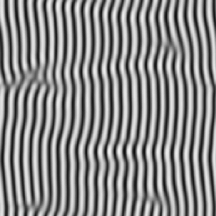
FIG. 4.: Pattern at $\bar{G}=0.7$, $f=4.0$, system size 128.0$\times$128.0 (grid spacing $h=0.5$), i.e., the lattice is 256$\times$256. $t=150.0$. Lengths are given in units of the (rescaled) diffusion length, times in units of the (rescaled) diffusion time.

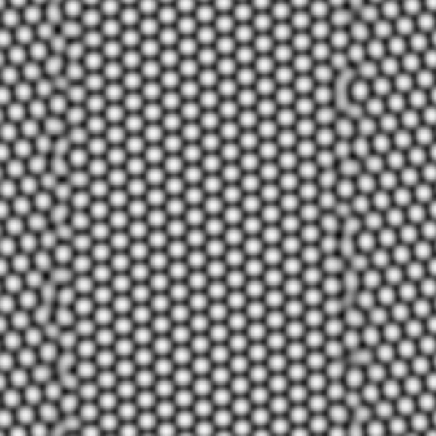
FIG. 5.: Pattern at $\bar{G}=0.6$, $f=2.0$, system size 128.0$\times$128.0 (grid spacing $h=0.5$). $t=2000.0$.

At smaller temperature gradients, flows of moderate size do not appear to strongly perturb the basic structure imposed by the MS instability. The dynamics is of course different, since the entire pattern drifts against the direction of the flow. Comparisons with simulations without flow show moreover that structures display more order (after the same time of dynamical evolution and starting from the same random initial conditions) with flow than they do without. As the flow is increased, new structures develop that we discuss below.

At $\bar{G}=0.35$, we find the flow to promote oscillatory structures. Figure 6 shows an example of a topologically ordered array of hexagons. Each cell has exactly six neighbors. The brightnesses of the cells indicate their different heights; white is high, black is low. Different sizes of the cells are due to their being in different phases of their basic oscillation. There is a phase shift of approximately $2\pi/3$ between neighboring cells. Phase coherence is not preserved throughout the entire array of cells as may be noted by comparison of the lower left and upper right parts of the pictures (not all big bright cells are exactly the same, and similar statements hold for the small bright cells and the dark cells). By animated visualization of a series of pictures, the oscillations are easily verified. Large cells are seen to become smaller and larger again, periodically. Small cells behave the same way, the only difference being a phase shift. Unfortunately, a movie cannot be transmitted in this media.

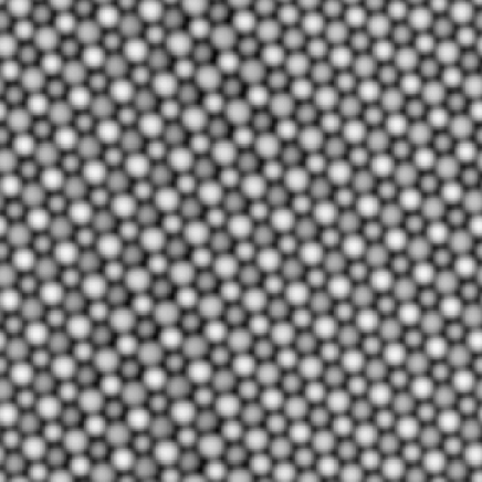
FIG. 6.: Pattern at $\bar{G}=0.35$, $f=2.0$, system size 128.0$\times$128.0 (grid spacing $h=0.5$). $t=2000.0$.

From earlier work [36], these oscillations are known to occur even without flow; an analytical discussion, not considering stability issues was given in [56]. For large grid spacings ($h=0.5$) we saw this dynamical state already at $\bar{G}=0.4$ with our finite-difference code. It was however observed to appear later, i.e., at smaller $\bar{G}$, when the mesh size was reduced, and we estimated the bifurcation to $2\pi/3$ oscillations to happen between $\bar{G}=0.4$ and $\bar{G}=0.35$ [36]. As it turns out, the spectral code with its higher accuracy does not yet produce the oscillations at $\bar{G}=0.35$, if flow is absent, but it does so in the presence of even small flows ($f=1.0$). In addition, the cellular lattice becomes more ordered, topological defects are eliminated more efficiently under flow.

To finish this introductory tour through parameter space, we consider a temperature gradient of $\bar{G}=0.25$ (Fig. 7), which was impossible to do with the finite-difference code because of numerical instabilities. Even with the spectral code we have to reduce the mesh size to obtain numerically stable results for $\bar{G}$ distinctly smaller than 0.35.

The example suggests that patterns are generically weakly turbulent at such a small gradient, i.e., they show time-dependent nonrelaxational behavior. Nevertheless, some ordering influence of the flow may be noted even here (cells tend to align along the direction perpendicular to the flow) and becomes much more conspicuous as the flow is increased, to the extent of rendering structures regular again at larger flows. We will return to this question in II.

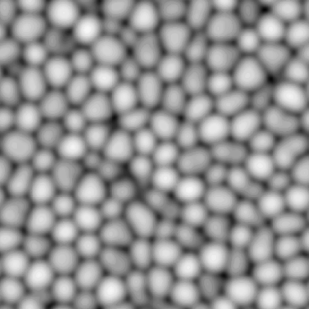
FIG. 7.: Pattern at $\bar{G}=0.25$, $f=2.0$, system size 76.8$\times$76.8 (grid spacing $h=0.3$). $t=1500.0$.

B Measured properties

In order to characterize the bifurcation from the planar front, we introduce the standard deviation $A\equiv\sqrt{\langle(\zeta-\langle\zeta\rangle)^{2}\rangle}$ as a measure for the amplitude of the steady state structure, reached in the late stage evolution of an initially sinusoidal interface. Figure 8 shows the amplitude so obtained as a function of the temperature gradient.

FIG. 8.: Amplitude $A$ of steady-state stripe patterns for a fixed flow of $f=2.0$ as a function of the temperature gradient. The initial condition was a sinusoidal pattern with wavenumber $0.98$, with the wave crests oriented parallel to the $y$ axis. Measurement of the amplitude was done after $t=1000.0$ in units of the (rescaled) diffusion time. The dotted line gives the theoretical position of the bifurcation point, according to Eq. (15).

Due to the small system size (16.0$\times$16.0), it was possible to keep stripe structures stable well below the threshold of the appearance of hexagons ($\bar{G}=2/3$). As expected [55], the bifurcation is supercritical.

In the presence of any nonzero flow, the basic structures appearing at the instability threshold are stripes rather than hexagons. Whereas our large-flow predictions, discussed below (and, in more detail, in II), might require some effort to be realized experimentally, this result should be of immediate experimental relevance, since it is valid no matter how small the flow. Extremely small flows would make the range of temperature gradients in which stripes dominate over hexagons very small, but this range would nevertheless be present and necessarily observed, at least temporarily, on crossing the bifurcation threshold via reduction of $\bar{G}$. Since the argument for the prevalence of stripes is drawn from linear stability analysis, it need not continue to hold, once amplitudes become large enough for nonlinearities to play an important role. In II, we will see that this indeed happens as long as the flow is not too strong. The transcritical nature of the bifurcation to hexagons will then turn out important.

Measuring the velocity of the interface for values of $\bar{G}$ which are sufficiently close to the instability threshold we find that it exhibits damped oscillations. Examples for $\bar{G}=0.7$ and $\bar{G}=0.6$ are presented in Fig. 9. Our discussion of the velocity measuring procedure in Sec. III suggests that this phenomenon may be due to some dynamics superimposed on the drift motion. This is corroborated by examining the frequency of oscillation.

FIG. 9.: Oscillations of the lateral pattern velocity after initialization with a random structure. Solid line: $\bar{G}=0.6$, dashed line: $\bar{G}=0.7$. For the smaller value of $\bar{G}$, the oscillations decay faster.

The figure shows clearly that the frequency is slightly higher for the larger value of $\bar{G}$ (for $\bar{G}=0.7$, there are 17 oscillations in the time window displayed, but only 16 for $\bar{G}=0.6$). A precise determination of the (angular) frequency reveals that it is very close to the (angular) frequency $\omega=\sqrt{8k\bar{G}}$ of homogeneous solutions [28] to Eq. (3). As has been noted before [28], patterns initiated close to the threshold $\bar{G}_{c}$ oscillate as a whole before settling down into a steady state.

The oscillatory velocity pattern is thus an effect of the temporal modulation of the pattern [similar to the $\cos\omega t$ term in Eq. (24)] and we should consider the average over these oscillations the true velocity. They are a nongeneric feature of the current amplitude equation (3), which is not shared by other equations such as the Kuramoto-Sivashinsky equation. For lower values of $\bar{G}$, these oscillations are not present.

Let us now look at the drift velocities measured for different values of the temperature gradient and the flow. Figure 10 collects some data corresponding to gradients between $\bar{G}=0.35$ and $\bar{G}=0.7$. For flow strengths below $|f|=6$, all the data points collapse approximately onto one curve. This is to be expected from the linear-stability result (B9), which shows that the $\bar{G}$ dependence of the drift velocity is weak for small $f$. The dashed line in the figure shows this result for $\bar{G}=0.6$.

On the other hand, the spreading of the data points for $f>6$ does not follow from the corresponding result (B20) for large $f$. Clearly, the linear theory breaks down here. As we shall see below, the deviation of the drift velocity from the analytic result happens in the vicinity of the transition to a new pattern, where the drift velocity is determined by nonlinear effects. We will discuss this in particular for one temperature gradient, but there seems to be a morphology transition in all cases where a strong deviation from the linear theory arises; the transition is not always to the same new pattern however. (For $\bar{G}=0.4$, there seem to be two transitions.)

FIG. 10.: Measured drift velocity as a function of the flow for different temperature gradients. Stars: $\bar{G}=0.7$, squares: $\bar{G}=0.6$, triangles: $\bar{G}=0.5$ (most of them covered by other symbols), inverted triangles: $\bar{G}=0.4$, circles: $\bar{G}=0.35$. Dashed line: Analytic velocity from linear stability analysis for $\bar{G}=0.6$.

Without flow, the equation of motion (3) is symmetric under the parity transformation $x\to-x$. Drifting patterns arise, because this symmetry is broken by the flow term, meaning that we do not have spontaneous symmetry breaking as, e.g., with parity breaking patterns in the purely diffusive case [56]. Whereas those patterns are not stable in extended systems, the present drifting structures are robust.

It is easy to see that flow-induced drifting cells must themselves be asymmetric with respect to a mirror plane parallel to the $yz$ plane, even though this asymmetry may be barely perceptible to the eye. To show this, we assume the opposite to be true, i.e., $\zeta$ to be symmetric under $x\to-x$. Transforming Eq. (3) to a comoving frame, which results in $\zeta_{t}\to\zeta_{t}-v\zeta_{x}$, we obtain from the antisymmetric part of the equation:

$$v\left(2+\frac{1}{k}+\nu\right)\nabla^{2}\zeta_{x}-f\frac{\partial}{\partial x}{\cal L}[\zeta]=-2v\zeta_{x}\nabla^{2}\zeta-2v\left(\left|\nabla\zeta\right|^{2}\right)_{x}\>.$$ (27)

But this relation must be invariant under an exchange of $x$ and $-x$ and a replacement of $v$ by $-v$. Hence, the flow term must vanish, which means it cannot play any role. This is in contradiction with the fact that drifting patterns on large scales are not observed in the absence of flow.

We have probed the asymmetry of cells in a number of different ways as a test of our numerical procedure. The most distinctive method was as follows: first the 2D interface was cut by a straight line parallel to the $x$ axis through the middle of a cell, to get its profile. Then the top part of the cell (everything above a chosen threshold height) was fitted to a parabola. The difference between the fit function and the actual cell profile is given for one case without and one with flow in Fig. 11. Evidently, this difference is symmetric in the former and asymmetric in the latter case. Since the flow comes from the left in the picture, we can moreover deduce that the cells are steeper on the upflow side than on the downflow one.

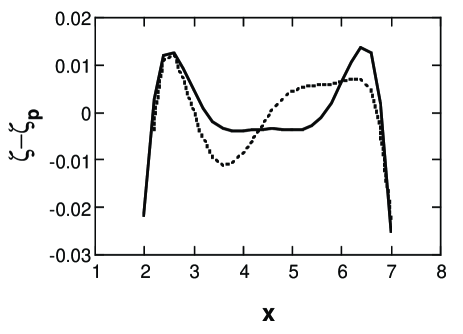
FIG. 11.: Deviation of the cell shape from a parabola, for a case without flow (solid line) and one with a flow $f=2.0$ (dashed line). $\bar{G}=0.5$.

V Conclusions

The addition of a shear flow to directional solidification near the absolute stability limit affects the system in several more or less profound ways.

First, the flow breaks the mirror symmetry of the equation of motion. This implies that cellular solutions are asymmetric in general. Symmetry breaking of this type is known to lead to drifting solutions in cases where it appears spontaneously [28, 56]. It produces the same behavior here. The appearance of a drift velocity can be understood at the level of a linear stability analysis which moreover provides a decent quantitative estimate for its value. As expected, this description of the drifting pattern breaks down for larger flows, where nonlinear effects exert a stronger influence.

Second, the patterns appearing at the instability threshold of the planar interface for $\bar{G}>\bar{G}_{c}(f=0)$ are not hexagons but stripes. We shall see that this statement will have to be made more precise in II, because at this moment, we cannot say anything about the stability of stripe structures. The planar front becomes unstable via a supercritical Hopf bifurcation. Since the transition to hexagons of the system without flow is transcritical, i.e., hexagons can exist even below the threshold of the diffusive instability, we may expect stripes and hexagons to interact, at least at small flow strengths. This point will be discussed in some detail in II.

The main effect of the flow in situations where a structure of hexagonal cells develops (i.e., for $\bar{G}<\bar{G}_{c}(f=0)$ and not too large a flow) is to promote ordering, i.e., the appearance of a hexagonal translational lattice. Hence, defects are eliminated more efficiently in the laterally moving pattern than in one at rest. Defects that stay tend to become aligned in the flow to give grain boundaries a preferential orientation (perpendicular to the flow). Finally, the flow increases instability towards local oscillations of cells with relative phase shifts. Since these oscillations also act to reduce the number of defects [36], the flow reinforces this tendency, again working to improve translational order.

Acknowledgments

This work was supported by a PROCOPE grant for travel exchanges by the DAAD (German academic exchange service), grant no. 9822777, and the Egide (corresponding French organisation), grant no. 01258ZD.

A Real space representation of the flow term

Since the nonlocal term is given by a product in Fourier space

$${\cal L}[\zeta]^{\ast}\equiv|{\bf p}|\,\zeta^{\ast}\>,$$ (A1)

(where for brevity we denote the Fourier transform by an asterisk) its position space expression can be obtained as a convolution integral. Care must be taken, however, because the inverse Fourier transform of $|{\bf p}|$ does not exist. Therefore, we first rewrite ${\cal L}[\zeta]^{\ast}$ as a different product.

For a one-dimensional interface, the most convenient approach seems to be to write

$${\cal L}[\zeta]^{\ast}=\hbox{sign}(p)p\,\zeta^{\ast}=-{\rm i}\,\hbox{sign}(p)(\partial_{x}\zeta)^{\ast}\>$$ (A2)

While the (inverse) Fourier transform of the sign function does not exist as a function, it is defined in the distribution sense and easily calculable:

$$s(x)\equiv\frac{1}{2\pi}\int_{-\infty}^{\infty}\hbox{e}^{{\rm i}\,px}\hbox{sign}(p)dp=\frac{1}{2\pi}\left(\int_{0}^{\infty}\hbox{e}^{{\rm i}\,px}dp-\int_{0}^{\infty}\hbox{e}^{-{\rm i}\,px}dp\right)=\frac{{\rm i}\,}{\pi}\frac{\cal P}{x}\>,$$ (A3)

the last expression being the distribution that is pointwise equal to ${\rm i}\,/\pi x$ but requires any integral in which it appears to be interpreted as a principal value.

Hence we obtain for the flow term in 1D:

$$-f\partial_{x}{\cal L}[\zeta]=-\frac{f}{\pi}\,\partial_{x}\mathop{\mathchoice{-\mskip-18.00003mu\int}{-\mskip-15.0mu\int}{-\mskip-15.50003mu\int}{-\mskip-15.50003mu\int}}\nolimits_{-\infty}^{\,\infty}d{x^{\prime}}\frac{1}{x-{x^{\prime}}}\partial_{{x^{\prime}}}\zeta({x^{\prime}})\>,$$ (A4)

where the bar indicates a principal value integral. More specifically, we define

$$\mathop{\mathchoice{-\mskip-18.00003mu\int}{-\mskip-15.0mu\int}{-\mskip-15.50003mu\int}{-\mskip-15.50003mu\int}}\nolimits_{-\infty}^{\,\infty}d{x^{\prime}}\ldots=\lim_{\epsilon\to 0^{+}}\left(\int_{-\infty}^{x-\epsilon}d{x^{\prime}}\ldots+\int_{x+\epsilon}^{\infty}d{x^{\prime}}\ldots\right)\>.$$ (A5)

For a two-dimensional interface, another decomposition is more appropriate

$${\cal L}[\zeta]^{\ast}=-\frac{1}{|{\bf p}|}(-{\bf p}^{2})\zeta^{\ast}=-\frac{1}{|{\bf p}|}(\nabla^{2}\zeta)^{\ast}\>\>.$$ (A6)

(In one dimension, the inverse Fourier transform of $1/|{\bf p}|$ is problematic because of the divergence at the origin, which in two dimensions is compensated by the volume element.) Hence we have

$${\cal L}[\zeta]=\int_{-\infty}^{\infty}dx^{\prime}\int_{-\infty}^{\infty}dy^{\prime}s({\bf x}-{\bf x^{\prime}}){\nabla^{\prime}}^{2}\zeta({\bf x^{\prime}})\>,$$ (A7)

where $[{\bf p}=(p_{x},p_{y})]$

$$s({\bf x}) = \frac{1}{4\pi^{2}}\int_{-\infty}^{\infty}dp_{x}\int_{-\infty}^{\infty}dp_{y}\frac{-1}{\sqrt{p_{x}^{2}+p_{y}^{2}}}\,\hbox{e}^{{\rm i}\,{\bf px}}$$ (A8)

$$= -\frac{1}{4\pi^{2}}\int_{0}^{2\pi}d\phi\int_{0}^{\infty}dp\frac{p}{p}\exp\left({\rm i}\,p|{\bf x}|\cos\phi\right)\>.$$ (A9)

To obtain the second expression, we have oriented the polar coordinate system such that the ray $\phi=0$ is parallel to ${\bf x}$ (hence ${\bf px}=p|{\bf x}|\cos\phi$). Therefore,

$$s({\bf x}) = -\frac{1}{4\pi^{2}}\int_{0}^{2\pi}d\phi\left(\frac{{\rm i}\,{\cal P}}{|{\bf x}|\cos\phi}+\pi\delta(|{\bf x}|\cos\phi)\right)$$ (A10)

$$= -\frac{{\rm i}\,}{4\pi^{2}\left|\bf x\right|}\mathop{\mathchoice{-\mskip-18.00003mu\int}{-\mskip-15.0mu\int}{-\mskip-15.50003mu\int}{-\mskip-15.50003mu\int}}\nolimits_{0}^{2\pi}d\phi\frac{1}{\cos\phi}-\frac{1}{4\pi}\int_{0}^{2\pi}d\phi\frac{1}{|{\bf x}||\sin\phi|}\left[\delta\left(\phi-\frac{\pi}{2}\right)+\delta\left(\phi-\frac{3\pi}{2}\right)\right]$$ (A11)

$$= -\frac{1}{2\pi|{\bf x}|}\>.$$ (A12)

The principal value integral of $1/\cos\phi$ vanishes as it extends over an entire period. Thus we arrive at the following final expression for the flow term

$$-f\partial_{x}{\cal L}[\zeta]=\frac{f}{2\pi}\,\partial_{x}\int_{-\infty}^{\infty}dx^{\prime}\int_{-\infty}^{\infty}dy^{\prime}\frac{1}{|{\bf x-x^{\prime}}|}{\nabla^{\prime}}^{2}\zeta({\bf x^{\prime}})\>.$$ (A13)

Both the 1D and 2D expressions clearly exhibit the nonlocality of the flow term and its odd parity symmetry. All the other terms in Eq. (3) have even parity, so the flow term provides a symmetry breaking mechanism.

Note also that the nonlocal kernels appearing in these expression are almost the simplest possible, if one thinks in terms of gradient expansions. Local terms produce successive powers of derivatives, corresponding to powers of ${\bf p}$ in Fourier space. Nonlocal terms would be connected with powers of $1/|{\bf p}|$, which must be compensated for (in order to keep things finite at small ${\bf p}$) by spatial derivatives.

B Analytic calculation of drift velocities

In order to solve Eqs. (21) and (22) analytically, we first cast them in a simpler form introducing

$$\tilde{\omega}_{r}=\omega_{r}+2q^{2}\>.$$ (B1)

This yields

$$\tilde{\omega}_{r}^{4}+\tilde{\omega}_{r}^{2}\left(8\bar{G}-q^{4}-8q^{2}\right)-\frac{f^{2}q^{4}}{4} = 0\>,$$ (B2)

$$f^{2}q^{2}\left(\tilde{\omega}_{r}-2q^{2}\right)-2\tilde{\omega}_{r}^{3}\left(4\tilde{\omega}_{r}-2q^{2}-8\right) = 0\>.$$ (B3)

We then consider the limiting cases $f\ll 1$ and $f\gg 1$. The first of these is very simple. As we know that there are solutions without flow, we set, as a first approximation, $f=0$ in Eqs. (B2) and (B3). $\omega_{i}$ will still remain $f$ dependent via (20), which takes the form

$$\omega_{i}=\frac{fq^{2}}{2\tilde{\omega}_{r}}\>.$$ (B4)

We get immediately

$$\tilde{\omega}_{r}=2+\frac{1}{2}q^{2}$$ (B5)

and the Eq. (B2) for $q$ can be reduced to quadratic. The result is

$$q^{2} = -4+\frac{4}{\sqrt{3}}\sqrt{4+2\bar{G}}\>,$$ (B6)

$$\omega_{r} = -2q^{2}+\frac{2}{\sqrt{3}}\sqrt{4+2\bar{G}}\>,$$ (B7)

$$\omega_{i} = f\left(1-\frac{\sqrt{3}}{\sqrt{4+2\bar{G}\vphantom{\bar{\bar{G}}}}}\right)\>,$$ (B8)

$$v=-\frac{\omega_{i}}{q} = -\frac{f\sqrt{3}}{2\sqrt{4+2\bar{G}\vphantom{\bar{\bar{G}}}}}\left(\sqrt{\frac{4+2\bar{G}}{3}}-1\right)^{1/2}\>.$$ (B9)

As an example, for $\bar{G}=0.7$, this gives a drift velocity $v=0.218f$, and the dependence on $\bar{G}$ is weak. Note that for this $\bar{G}$ value $\omega_{r}<0$ and hence the structure will decay to a planar front (moving along as it does so at the the calculated velocity).

The case $f\gg 1$ is slightly more complicated. Considering (B2) and the fact that $\bar{G}$ is of order 1 in the interesting parameter range, we see (from the signs in the equation) that the only possible dominant balance for a pair of terms is

$$\tilde{\omega}_{r}^{4}\sim\frac{f^{2}q^{4}}{4}\>.$$ (B10)

Inserting this in (B3) and combining the two equations, we find however

$$\tilde{\omega}_{r}\sim 2q^{2}\>,$$ (B11)

which is in contradiction with (B10) for $f\gg 1$ and $q=O(1)$. This implies that dominant balances in (B2) must contain three terms at least and that the wavenumber $q$ of the fastest-growing mode has to scale, too. It must increase with $f$ and Eqs. (B10) and (B11) suggest the scaling $f\sim q^{2}$. Hence, we set

$$f=aq^{2}\>,$$ (B12)

assuming $a=O(1)$. Inserting this into Eqs. (B2) and (B3) and using $q\gg 1$, we arrive at

$$\tilde{\omega}_{r}^{4}-\tilde{\omega}_{r}^{2}q^{4}-\frac{a^{2}q^{8}}{4} = 0\>,$$ (B13)

$$a^{2}q^{6}(\tilde{\omega}_{r}^{2}-2q^{2}) = 8\tilde{\omega}_{r}^{4}-4\tilde{\omega}_{r}^{3}q^{2}\>.$$ (B14)

Equation (B13) can be solved for $\tilde{\omega}_{r}^{2}$:

$$\tilde{\omega}_{r}^{2}=\frac{q^{4}}{2}\left(1+\sqrt{1+a^{2}}\right)\>.$$ (B15)

Using this in (B14), we end up, after some simplifications, with a relation determining $a$:

$$\frac{\sqrt{2}}{8}\left(1+\sqrt{1+a^{2}}\right)^{3/2}-\sqrt{1+a^{2}}=0\>.$$ (B16)

The numerical solution of this algebraic equation yields $a=28.88$. (There is only one real solution.) We then obtain

$$q = \sqrt{\frac{f}{a}}\approx 0.186\sqrt{f}\>,$$ (B17)

$$\omega_{r} = \left(\sqrt{\frac{1+\sqrt{1+a^{2}}}{2}}-2\right)\frac{f}{a}\approx 0.065f\>,$$ (B18)

$$\omega_{i} = \frac{2f}{\sqrt{2\left(1+\sqrt{1+a^{2}}\right)}}\approx 0.129f\>,$$ (B19)

$$v = -\frac{\omega_{i}}{q}\approx-0.695\sqrt{f}\>.$$ (B20)

All of these expressions are independent of $\bar{G}$, as they must, being leading order results for $f\gg\bar{G}$.

REFERENCES

- [1] W.W. Mullins and R. F. Sekerka, J. Appl. Phys. 325, 444 (1964).
- [2] K.A. Jackson and J.D. Hunt, Met. Trans. AIME 236, 1129 (1966).
- [3] K.A. Jackson and J.D. Hunt, Acta Metall. 13, 1212 (1965).
- [4] R. Trivedi and K. Somboonsuk, Acta Metall. 33, 1061 (1985).
- [5] S. de Cheveigné, C. Guthmann, and M. M. Lebrun, J. Phys. France 47, 2095 (1986).
- [6] S. de Cheveigné, C. Guthmann, P. Kurowski, E. Vicente, and H. Biloni, J. Cryst. Growth 92, 616 (1988).
- [7] P. Kurowski, C. Guthmann, and S. de Cheveigné, Phys. Rev. A 42, 7368 (1990).
- [8] S. de Cheveigné and C. Guthmann, J. Phys. I France 2, 193 (1992).
- [9] M.H. Burden and J.D. Hunt, J. Cryst. Growth 22, 99 (1974), J. Cryst. Growth 22, 109 (1974).
- [10] M. Zimmermann, M. Carrard, and W. Kurz, Acta Metall. 37, 3305 (1989).
- [11] H. Nguyen Thi, B. Billia, Y. Dabo, D. Camel, B. Drevet, M.D. Dupouy, and J.J. Favier, in Proc. Xth European and VIth Russian Symp. Physical Sciences in Microgravity, eds. V.S. Avduyevsky and V.I. Polezhaev (Association for the Promotion of Conversion, Moscow, 1997).
- [12] M.D. Dupouy, D. Camel, F. Botalla, J. Abadie, and J.J. Favier, in Proc. of Melding, Welding and Advanced Solidification Processes, eds. B.G. Thomas and C. Beckermann (TMS, Warrendale, 1998).
- [13] N. Noël, PhD thesis, Université d’Aix-Marseille III, 1996. N. Noël, H. Jamgotchian, and B. Billia, J. Cryst. Growth 181, 117 (1997).
- [14] N. Noël, H. Jamgotchian, and B. Billia, J. Cryst. Growth 187, 516 (1998).
- [15] B. Caroli, C. Caroli, and B. Roulet, J. Phys. France 43, 1767 (1982).
- [16] D. J. Wollkind, D. B. Oulton, and R. Sriranganathan, J. Phys. France 45, 505 (1984).
- [17] L. H. Ungar and R. A. Brown, Phys. Rev. B 29, 1367 (1984), Phys. Rev. B 30, 3993 (1984), Phys. Rev. B 31, 5931 (1985). L. H. Ungar, M. J. Bennett, and R. A. Brown, Phys. Rev. B 31, 5923 (1985).
- [18] T. Dombre and V. Hakim, Phys. Rev. A 36, 2811 (1987).
- [19] M. Ben Amar and B. Moussallam, Phys. Rev. Lett. 60, 317 (1988).
- [20] D. A. Kessler and H. Levine, Phys. Rev. A 39, 3041 (1989).
- [21] K. Brattkus and C. Misbah, Phys. Rev. Lett. 64, 1935 (1990).
- [22] H. Levine and W. Rappel, Phys. Rev. A 42, 7475 (1990).
- [23] C. Misbah, H. Müller-Krumbhaar, and Y. Saito, J. Cryst. Growth 99, 156 (1990).
- [24] A. Classen, C. Misbah, H. Müller-Krumbhaar, and Y. Saito, Phys. Rev. A 43, 6920 (1991).
- [25] K. Kassner, C. Misbah, and H. Müller-Krumbhaar, Phys. Rev. Lett. 67, 1551 (1991).
- [26] A. Valance, K. Kassner, and C. Misbah, Phys. Rev. Lett. 69, 1544 (1992).
- [27] W.-J. Rappel and H. Riecke, Phys. Rev. A 45, 846 (1992).
- [28] K. Kassner, C. Misbah, H. Müller-Krumbhaar, and A. Valance, Phys. Rev. E 49, 5477, (1994), ibid. 5495 (1994).
- [29] M. Ben Amar and E. Brener, Phys. Rev. Lett. 71, 589 (1993).
- [30] E. Brener, Phys. Rev. Lett. 71, 3653 (1993).
- [31] E. Brener and D. Temkin, Phys. Rev. E 51, 351 (1995).
- [32] R. Kobayashi, Experimental Mathematics 3, 59 (1994).
- [33] A. Karma and W. Rappel, Phys. Rev. Lett. 77, 4050 (1996), Phys. Rev. E 57, 4323 (1998).
- [34] T. Abel, E. Brener, and H. Müller-Krumbhaar, Phys. Rev. E 55, 7789 (1997).
- [35] B. Grossmann, K.R. Elder, M. Grant, and J.M. Kosterlitz, Phys. Rev. Lett. 71, 3323 (1993).
- [36] K. Kassner, J.-M. Debierre, B. Billia, N. Noël, and H. Jamgotchian, Phys. Rev. E 57, 2849 (1998).
- [37] A.J. Simon, J. Bechhoefer, and A. Libchaber, Phys. Rev. Lett. 63, 2574 (1988).
- [38] A.J. Simon and A. Libchaber, Phys. Rev. A 41, 7090 (1989).
- [39] J.-M. Flesselles, A.J. Simon, and A. Libchaber, Adv. Phys. 40, 1 (1991).
- [40] In [36], structures were simulated up to 250 000 rescaled diffusion times . For typical solids, with s (cm2/s, m/s), whereas for liquid crystals, s is achievable (cm2/s, m/s).
- [41] H. Jamgotchian, B. Billia, F. Zamkotsian, and R. Guérin, in Proceedings of the 2nd European Symposium on the Utilisation of the Space Station, (ESTEC, Nordwijk, The Netherlands, ESA SP-433, Feb. 1999), p. 329.
- [42] S.H. Davis, J. Fluid Mech. 212, 241 (1990).
- [43] A.K. Hobbs and P. Metzener, J. Crystal Growth 118, 319 (1992).
- [44] K. Kassner, A.K. Hobbs, and P. Metzener, Physica D 93, 23 (1996).
- [45] M.J. Aziz, J. Appl. Phys. 53, 1158 (1982).
- [46] Y. Marietti, J.-M. Debierre, K. Kassner, and T. Bock, Phys. Rev. E, this volume, page …
- [47] K. Kassner, Pattern formation in diffusion-limited crystal growth (World Scientific, Singapore, 1996).
- [48] S.R. Coriell, M.R. Cordes, W.S. Boettinger, and R.F. Sekerka, J. Cryst. Growth 49, 13 (1980).
- [49] D.T.J. Hurle, E. Jakeman, and A.A. Wheeler, J. Cryst. Growth 58, 163 (1982).
- [50] D.T.J. Hurle, E. Jakeman, and A.A. Wheeler, Phys. Fluids 26, 624 (1983).
- [51] S.R. Coriell, G.B. McFadden, G.B. Boisvert, and R.F. Sekerka, J. Cryst. Growth 69, 514 (1984).
- [52] B. Caroli, C. Caroli, C. Misbah, and C. Roulet, J. Phys. Paris 46, 401 (1985).
- [53] D.S. Riley and S.H. Davis, Applied Mathematics Technical Report No. 8838 (Northwestern University, 1989).
- [54] S.A. Forth and A.A. Wheeler, J. Fluid Mech. 202, 339 (1989).
- [55] A.K. Hobbs and P. Metzener, J. Crystal Growth 112, 539 (1991).
- [56] I. Daumont, K. Kassner, C. Misbah, and A. Valance, Phys. Rev. E 55, 6902 (1997).
- [57] Note that absolute instability as used in this paragraph is a concept entirely different from that of the absolute stability limit (sometimes in short denoted as absolute stability) as referred to in the remainder of the paper. The former notion applies to arbitrary systems with traveling wave instabilities. If they are absolutely unstable, a localized perturbation will grow at any fixed position where it was originally created. On the other hand, if a localized perturbation grows only in a comoving frame of reference, while being advected away with its tail at its original position decaying, one speaks of convective instability (only). Linear instability implies at least convective instability, but not necessarily absolute instability. On the other hand, the notion of an absolute stability limit in the context of directional solidification simply means the threshold velocity above which a planar interface is stabilized by surface tension even in the absence of a thermal gradient.