Magnetotunneling spectroscopy of mesoscopic correlations
in two-dimensional electron systems

Abstract

An approach to experimentally exploring electronic correlation functions in mesoscopic regimes is proposed. The idea is to monitor the mesoscopic fluctuations of a tunneling current flowing between the two layers of a semiconductor double-quantum-well structure. From the dependence of these fluctuations on external parameters, such as in-plane or perpendicular magnetic fields, external bias voltages, etc., the temporal and spatial dependence of various prominent correlation functions of mesoscopic physics can be determined. Due to the absence of spatially localized external probes, the method provides a way to explore the interplay of interaction and localization effects in two-dimensional systems within a relatively unperturbed environment. We describe the theoretical background of the approach and quantitatively discuss the behavior of the current fluctuations in diffusive and ergodic regimes. The influence of both various interaction mechanisms and localization effects on the current is discussed. Finally a proposal is made on how, at least in principle, the method may be used to experimentally determine the relevant critical exponents of localization-delocalization transitions.

PACS numbers: 73.21.-b, 73.23.Hk, 73.40.Gk, 73.50.-h

I Introduction

At low temperatures, disordered or chaotic electronic systems are strongly affected by mechanisms of quantum interference. These interference effects manifest themselves in anomalously strong fluctuations of both thermodynamic and transport observables and in the spatial localization of quantum mechanical wave functions [1]. They find their common origin in an interplay of the classical nonintegrability of the charge carrier dynamics and the wave nature of quantum mechanical propagation. To quantitatively characterize this ‘mesoscopic’ behavior, one commonly employs correlation functions of the type

$$F({\bf x}_{1},{\bf x}_{2},{\bf x}_{3},{\bf x}_{4};\omega,\Delta\alpha)\equiv$$

$$\qquad\equiv\langle G^{-}({\bf x}_{1},{\bf x}_{2};\epsilon,\alpha)G^{+}({\bf x}_{3},{\bf x}_{4};\epsilon+\omega,\alpha+\Delta\alpha)\rangle\,,$$

where $G^{\pm}$ is the retarded/advanced single-particle Green function. Here $\langle\dots\rangle$ stands for some kind of averaging (e.g., averaging over realizations of disorder) and the parameter $\alpha$ symbolically represents an optional dependence of the Green function on external control parameters (magnetic fields, gate voltages or others). Correlation functions of this type appear as the ‘most microscopic’ building block in the analysis of the majority of fluctuating mesoscopic observables. As a consequence of constructive quantum interference these objects become long ranged whenever the spatial arguments ${\bf x}_{1},\dots,{\bf x}_{4}$ are pairwise close (on scales of $l_{\rm min}$, the range of the averaged Green functions $\langle G^{\pm}\rangle$). Specifically,

• For ${\bf x}\equiv{\bf x}_{1}\approx{\bf x}_{2}$ and ${\bf x}^{\prime}\equiv{\bf x}_{3}\approx{\bf x}_{4}$, $F^{[d]}({\bf x},{\bf x}^{\prime})\equiv F({\bf x},{\bf x},{\bf x}^{\prime},{\bf x}^{\prime})$ describes the fluctuations of the (local) density of states (DoS), and, thus, the thermodynamic fluctuations and parametric correlations.

• For $\Delta\alpha=0$, $F^{[D]}({\bf x},{\bf x}^{\prime})\equiv F({\bf x},{\bf x}^{\prime},{\bf x}^{\prime},{\bf x})$ describes the total probability of propagation from ${\bf x}$ to ${\bf x}^{\prime}$. This is the generalized ‘diffuson’, a quantity of key relevance in the context of mesoscopic transport.

• Finally, in a system with unbroken time reversal symmetry, $F^{[C]}({\bf x},{\bf x}^{\prime})\equiv F({\bf x},{\bf x}^{\prime},{\bf x},{\bf x}^{\prime})$, the cooperon, becomes long ranged, too.

The dependence of the correlators $F^{[d;D;C]}$ on the long-ranged distance $r\equiv|{\bf x}-{\bf x}^{\prime}|$, the energy difference $\omega$, and $\Delta\alpha$ fundamentally characterizes a multitude of mesoscopic phenomena [1]. For this reason, many theoretical investigations in mesoscopic physics concentrate on an analysis of these objects. Experimentally, however, it has proven difficult to access the correlation functions $F^{[d;D;C]}$ directly: Ideally, one would like to continuously measure the dependence of the correlators $F^{[d;D;C]}$ over a range of at least the parameters $r$ and $\omega$. Irritatingly, this cannot be achieved within experimental setups based on a standard device-contact-electron system architecture. In fact, the mere presence of local contacts introduces an entire spectrum of difficulties obstructing the continuous experimental spectroscopy of transport and spectral correlation functions: First, the fixed attachment of local current/voltage electrodes prevents one from continuously monitoring the scale ($r$) dependence of transport correlation functions. This problem does not exist in measurements based on local tunneling tips [2]. In those, however, the electronic state of the tunneling device as well as its coupling to the electron system have to be precisely known to draw quantitatively reliable conclusions on the nature of the bulk electronic correlations of the latter. In particular, the distance between the device and the electron system has to be kept constant with atomic precision. These conditions can hardly be met under realistic conditions. Second, both local contacts and tunneling tips tend to disturb the electron system under investigation. In interacting systems, they lead to various manifestations of the orthogonality catastrophe. As a consequence, much of the measured current/voltage characteristics describes the process of local accommodation of charge carriers at the interface, rather than the electronic correlations of the bulk system. Third, a division between system and contacts of a mesoscopic conductor is, to a large extent, arbitrary. Quantum interference phenomena in mesoscopic systems tend to be highly nonlocal in space, and often it is not clear, where the physical processes responsible for the outcome of an experiment took place, in the ‘device’, the ‘contacts’, or all over the place.

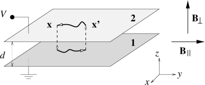
FIG. 1.: Schematic setup of the approach: two parallel two-dimensional electron systems are subject to a bias voltage and external magnetic fields. A tunneling current flowing between the layers is recorded as a function of the external control parameters.

These problems with contacted systems and local tunneling devices led to the idea to use a second electron system with essentially known properties as an extended tunneling spectroscope [3]. Setups of such type can conveniently be realized in double-quantum-well structures embedded in semiconductor heterostructures [4], as shown schematically in Fig. 1: Two electron systems confined in parallel wells separated by an isolating barrier of uniform thickness $d\sim 10-20$ nm form a double-layer system of two two-dimensional electron systems. A tunneling current $I$ from one layer to the other is driven by applying a voltage difference $V$ between them. The tunneling region is typically a few $100\times 100$ $\mu$m² in extent. In the absence of any disorder scattering and/or tunneling amplitude inhomogeneities, the tunneling from one layer to the other can only occur if energy and momentum are conserved. This leads to the resonant behavior of the tunneling current that is characteristic of two-dimensional systems. More generally, for constrained geometries (e.g., quantum wire/two-dimensional electron system) the field dependence of these resonances can be analyzed to obtain information on the dispersion of the fundamental excitations in the two systems [5].

However, in ‘real’ systems, inhomogeneities in the tunneling barrier thickness, static disorder, and other non-momentum conserving imperfections will lead to modifications of the idealized resonant current profile. Of these intruding mechanisms, the first appears to be the most serious: the current will respond with exponential sensitivity to any fluctuations of the layer separation; for strong enough spatial variations one may run into a scenario, where tunneling occurs only at a sparse set of ‘hot spots’, with no traces of a resonant profile left[6]. (Some characteristics of this type of current flow will be discussed below.) However, recent technological advances have made it possible to manufacture double-well systems with near-monolayer precision. In such devices, fluctuations in the tunneling matrix elements are reduced down to values of ${\cal O}(10\%)$ [7] and can be absorbed into a renormalization of the effective in-plane disorder. In the present paper, the focus will be on transport in these near-planar devices.

Even if the tunneling is homogeneous, static disorder will broaden the resonant behavior and introduce fluctuations. The broadening of the average current is related to the dynamics on short time scales [8]. In contrast, the fluctuations contain information about physical processes on much larger time scales [9] of the order of, e.g., the diffusion time through the system. It is the purpose of this paper to investigate the nature of these fluctuations and their relation to the aforementioned electronic correlation functions.

In fact, we will see below that detailed information on the correlation functions $F^{[d;D;C]}$ can be extracted from the tunneling current fluctuations without disturbing the system. Moreover, (i) the tunneling takes place uniformly at all points of the layers which means that an averaging over spatially fluctuating structures (e.g., details of the microscopic wave function amplitudes) is intrinsic to the data contained in the current. (ii) Several parameters can be tuned to gain information: The bias voltage resolves energetic correlations, a parallel magnetic field resolves spatial correlations, and a perpendicular magnetic field may serve as a control parameter for parametric correlations (i.e., correlations between Green functions evaluated at different values of external control parameters). (iii) The geometry of the layers can be designed freely, so that it is possible to study different regimes of particle dynamics (e.g., ergodic, ballistic, diffusive, etc.).

In this work, after the introduction of the general theoretical background of the tunneling current statistics, we will consider two prototypical system classes. First, we study extended systems for which the phase coherence length $L_{\phi}$ is much larger than the microscopic length $l_{\rm min}$ and a crossover or a transition from diffusive motion to Anderson localization may take place. For such systems, a parallel magnetic field ${\bf B}_{\parallel}$ can be employed as an instrument for resolving the long-range behavior of the correlation functions $F^{[D;C]}$. Importantly, the field alignment parallel to the two-dimensional planes implies that the charge carrier dynamics is not affected by ${\bf B}_{\parallel}$. While in the diffusive regime explicit expressions for the correlation functions are known, no quantitative expressions for regimes with strong (nonperturbative) localization and interaction effects are available. However, in a regime of localization-delocalization crossover or transition, scaling behavior is expected to restrict the functional form of $F^{[D;C]}$. This opens the possibility to extract the relevant critical indices from tunneling conductance measurements.

Second, we study a geometry, where one of the layers forms a ballistic quantum dot ($L<l_{\rm min}$) in the ergodic regime. The other, extended, layer serves as the spectrometer. For the quantum dot, the parametric correlations with respect to a perpendicular magnetic field, present in $F^{[d;D;C]}$, can be obtained from the current fluctuations. A similar setup has already been realized experimentally by Sivan et al. [10]. In that work, a single level (in contrast to our extended system) was used as a spectrometer to study a quantum dot device. This experiment led to results for the functional form of the correlator $F^{[d]}$, compatible with theoretical predictions from random matrix theory. However, one would expect that the data obtained from single-level spectroscopy is still weighted with nonuniversal wave-function amplitudes specific to the isolated ‘monitor level’. In contrast, for the two-dimensional layer/quantum dot setup considered here, the current flow is extended and spatially uniform. As a consequence, the tunneling current fluctuations are microscopically related to the purely spectral content of parametric correlations. Below we will establish the quantitative connection between the field and voltage dependence of the tunneling current fluctuations and a number of correlation functions that have been analyzed in the recent theoretical literature [11]. Moreover, we will try to assess to what extent these connections, obtained for the chaotic noninteracting electron gas, may be susceptible to interaction mechanisms such as Coulomb drag[12, 13] or Coulomb blockade effects [14].

The outline of the paper is as follows: In Sec. II we specify our model and review the general formula for the tunneling current. Turning to new results, we show that the Fourier transform of the tunneling conductance correlator with respect to the magnetic field directly yields the spatially resolved correlation functions $F^{[D;C]}$. In Sec. III the theory will be applied to diffusive and anomalous diffusive systems, and in Sec. IV to an analysis of spectral and parametric correlations in finite quantum dots. The impact of Coulomb charging effects on the tunneling current fluctuations will be discussed in Sec. IV. We conclude in Sec. V.

II Theory of tunneling currents

A The current formula

Consider a double-layer system consisting of two parallel two-dimensional electron gases (2DEGs), labelled 1 and 2, respectively (see Fig. 1). The two layers are separated by a tunneling barrier that we assume to be uniform. We aim to analyze the tunneling current $I$ under conditions, where the tunneling is weak (in a sense to be specified momentarily). After matching the electron densities in both layers by adjusting their chemical potential $\mu$, the current becomes a function of bias voltage $V$, temperature $T$, and, optionally, a magnetic field ${\bf B}$, $I=I(V,{\bf B};T,\mu)$.

Quantum mechanically, the system can be represented in terms of a tunneling Hamiltonian, $H=H_{1}+H_{2}+H_{\cal T}$, where $H_{1}$ and $H_{2}$ describe layer 1 and 2, respectively, while $H_{\cal T}$ describes the transfer of electrons between the layers [15]. Choosing a gauge where the bias voltage has been transferred to the tunneling matrix elements, $H_{\cal T}$ can be written as

$$H_{\cal T}=\int\!d^{2}x\,d^{2}x^{\prime}\left({\cal T}_{{\bf x}{\bf x}^{\prime}}e^{-iVt}{\psi^{\dagger}}_{1}({\bf x})\psi_{2}({\bf x}^{\prime})+{\rm h.c.}\right)\,,$$ (1)

where ${\cal T}_{{\bf x}{\bf x}^{\prime}}$ is the tunneling amplitude from ${\bf x}$ in layer 1 to ${\bf x}^{\prime}$ in layer 2, and $\psi^{\dagger}_{j}$, $\psi_{j}$ are electron creation and annihilation fields for layer $j=1,2$. For convenience, we use units where $\hbar\!=\!c\!=\!k_{\rm B}\!=\!e\!=\!1$. Since the tunneling matrix elements ${\cal T}_{{\bf x}{\bf x}^{\prime}}$ decrease exponentially (on atomic scales) as a function of $|{\bf x}-{\bf x}^{\prime}|$ we model ${\cal T}_{{\bf x}{\bf x}^{\prime}}$ as a spatially local object, ${\cal T}_{{\bf x}{\bf x}^{\prime}}={\cal T}_{{\bf x}}\delta({\bf x}-{\bf x}^{\prime})$. In the weak tunneling regime, i.e., when the typical time after which an electron tunnels is larger than the characteristic time scale that is to be resolved in the experiment, single-tunneling events dominate [16]. Then, the tunneling current reads [17, 8]

$$I(V,{\bf B}) = 2\int\!d^{2}x\,d^{2}x^{\prime}\int\!(d\epsilon^{[V]})\,{\cal T}_{{{\bf x}}}{\cal T}^{*}_{{{\bf x}^{\prime}}}\,e^{{i}{{\bf q}}({{\bf x}}-{{\bf x}^{\prime}})}\times$$ (3)

$$\times\,A_{1}({{\bf x}},{{\bf x}^{\prime}};\epsilon,{B_{\perp}})A_{2}({{\bf x}^{\prime}},{{\bf x}};\epsilon-V,{B_{\perp}})\,,$$

with the abbreviation $\int(d\epsilon^{[V]})=\int_{-\infty}^{\infty}\!\frac{d\epsilon}{2\pi}[n_{\rm F}(\epsilon-V)-n_{\rm F}(\epsilon)]$. Here $n_{\rm F}(\epsilon)=(1+e^{(\epsilon-\epsilon_{\rm F})/T})^{-1}$ is the Fermi distribution function at temperature $T$ and Fermi energy $\epsilon_{\rm F}$. The characteristic momentum scale set by the parallel field is ${\bf q}=d{\bf B}_{\parallel}\times{\bf e}_{z}$, where ${\bf e}_{z}$ is the unit vector perpendicular to the plane.

In Eq. (3) the quantities of main interest are the spectral functions of layer $j$, $A_{j}=i(G_{j}^{+}-G_{j}^{-})$, where $G_{j}^{\pm}$ is the retarded/advanced one-particle Green function. These spectral functions depend on the bias voltage $V$ applied to layer 2, and on the perpendicular magnetic field ${B_{\perp}}$. In fact, it will be our main objective to obtain information on these objects through their parameter dependences. In this context, it is crucial to note that ${\bf B}_{\parallel}$ does not change the dynamics within the individual layers, but merely weighs the tunneling current with an Aharonov-Bohm-type phase. The sensitivity of the current to this flux will help to gain information about the long-range propagation within the layers. A caricature of the basic idea is depicted in Fig. 1. This figure illustrates the basic physical processes underlying the current flow as described by Eq. (3): An electron tunnels at point ${{\bf x}}$ from layer 2 to 1, leaving a hole behind. It propagates within that layer to point ${{\bf x}^{\prime}}$, where it tunnels back to layer 2 and recombines with the hole. The in-plane magnetic field enters the formula via the flux through this electron-hole loop. Therefore, the in-plane magnetic field dependence of the tunneling current contains information about the typical area enclosed in the loop that in turn is determined by the typical range of propagation within the layers.

To further simplify the analysis, we note that in the absence of significant interaction corrections the spectral functions themselves do not exhibit temperature dependence. Under these conditions, a simple integral relation between currents at zero and finite temperatures holds:

$$I(T,\epsilon_{\rm F})=-\int\!d\epsilon\,\left(\frac{\partial n_{\rm F}}{\partial\epsilon}\right)I(T=0,\epsilon_{\rm F}=\epsilon)\,.$$ (4)

In the following, unless stated otherwise, all results will be given for $T=0$ only. The generalization to finite temperature – essentially a smearing of the $T=0$ results – obtains from Eq. (4).

In this paper, we are primarily interested in the tunneling current flowing between disordered systems. The microscopic properties of these systems will be described by some disorder distribution function about which we make three idealizing assumptions:

(1) The disorder potentials of the two layers are essentially uncorrelated [18].

(2) The e-e interaction and higher order tunneling processes are not able to introduce significant interlayer correlations in the motion of the charge carriers. Practically, this means that impurity averages can be taken for each layer independently. Roughly speaking, e-e interaction effects can be divided into three groups: momentum transfer between the layers (‘Coulomb drag’), charging effects associated with the tunneling process, and self-energy corrections (due to inelastic scattering and dephasing). Sizable interlayer Coulomb correlations may arise in very clean systems subject to strong perpendicular magnetic fields. In such systems, the e-e interaction can stabilize a fractional quantum Hall phase [19] and interlayer e-e interactions lead to additional correlation phenomena (spontaneous coherence and quantum Hall ferromagnets [20]). In contrast, for strong enough disorder, the e-e interaction is less significant [21] and, thus, the effective random potentials in each layer can be treated as statistically independent of each other. This assumption can be tested experimentally, as will be discussed below. Charging effects will inevitably influence the tunneling current at low bias; we postpone a discussion of these corrections until Sec. II B.

(3) Disorder does not significantly affect the spatial homogeneity of the tunneling, i.e. the tunneling matrix elements do not depend on position, ${\cal T}_{\bf x}\equiv{\cal T}$. The spatial homogeneity of the tunneling is very sensitive to the thickness of the barrier. However, it is now possible to grow heterostructures with near-monolayer precision and, thus, achieve a tunneling probability that is almost spatially constant [22, 23]. (In high precision devices, the space dependent relative fluctuations in the tunneling probability can be reduced to about 10% and lower [7].) The validity of this assumption can be tested experimentally. In the extreme case, where tunneling occurs only through tunneling centers or ‘pinholes’ [6], the resonant behavior of the tunneling current disappears. If the spacing between pinholes exceeds the mean free path, the average current is just proportional to the product of the local densities of states, $\langle I\rangle\sim\nu_{1}\nu_{2}$, and, furthermore, becomes independent of magnetic field.

In principle, a full (angle-resolved) analysis of the field dependence of the current would allow one to extract information about the distribution of tunneling centers [24]. However, further discussion of this type of ‘tunneling center spectroscopy’ is beyond the scope of this paper. Keeping in mind that the working assumption of near-homogeneous tunneling can be put to experimental test, we hereafter concentrate on the case ${\cal T}_{\bf x}\equiv{\cal T}$. (Note that, although significant inhomogeneities would largely obstruct the detection of transport correlations, they only have a minor effect on the analysis of spectral correlations.)

B Average current

To foster the discussion of fluctuations below, this section briefly recapitulates the main characteristics of the average tunnel current [25]. Under the assumptions formulated above it is given by

$$\langle I(V,{{\bf B}})\rangle = \frac{L^{2}}{\pi}\left|{\cal T}\right|^{2}\int\limits_{0}^{V}\!d\epsilon\int\!d^{2}x\,e^{i{\bf q}{\bf x}}\times$$ (6)

$$\times\langle A_{1}({\bf x};\epsilon,B_{\perp})\rangle\langle A_{2}(-{\bf x};\epsilon-V,B_{\perp})\rangle\,.$$

The current, Eq. (6), is characterized by the averaged one-particle Green function $\langle{G^{\pm}}_{j}({\bf x},{\bf x}^{\prime};\epsilon)\rangle$. This quantity is short-ranged on a scale $l_{\rm min}$. For small perpendicular magnetic fields $B_{\perp}$, $l_{\rm min}$ is set by the mean free path $l=v_{\rm F}\tau$, where $v_{\rm F}$ is the Fermi velocity and $\tau$ the elastic scattering time. (In cases, where the scattering times in the layers are different, we need to generalize to $\tau_{j}$, $j=1,2$.) We here focus on systems, where the mean free path $l$ is much shorter than the linear system size $L$ [26]. For stronger perpendicular magnetic fields, with cyclotron frequency $\omega_{c}=B_{\perp}/m$ exceeding the inverse elastic scattering rate $\tau^{-1}$, the classical cyclotron radius $R_{c}=v_{\rm F}/\omega_{c}$ is smaller than the mean free path $l$ implying that $l_{\rm min}=R_{c}$ (see, e.g., Ref. [27]).

The average current has been studied theoretically [8] and experimentally [22, 23]. For matched Fermi energies and vanishing magnetic fields, the theoretical result reads

$$\frac{\langle I(V,{\bf B}=0)\rangle}{V}=G_{0}\frac{\Gamma^{2}}{V^{2}+\Gamma^{2}}\,,\qquad G_{0}=\frac{2\nu|{\cal T}|^{2}}{\Gamma}L^{2}\,,$$ (7)

where $\Gamma=\Gamma_{1}+\Gamma_{2}$, $\Gamma_{j}=1/(2\tau_{j})$ is the line-width of the Lorentzian-shaped average spectral function in layer $j$, $\nu$ is the single-particle-level density of states per unit area, and $G_{0}$ is the characteristic low-bias average conductance of the system. For the average current, the condition of weak tunneling is

$$\Gamma_{\cal T}<\Gamma\,,$$ (8)

where $\Gamma_{\cal T}\equiv\left|{\cal T}\right|^{2}\Gamma^{-1}$ is the inverse of the (golden rule) rate at which a particle propagating in one layer tunnels to the other. Henceforth we will focus on the regime of small bias voltage $V\ll\Gamma$. Under these conditions, $\langle I(V,{\bf B}=0)\rangle/V\approx G_{0}$. In the presence of a moderately weak in-plane magnetic field ($|{\bf q}|^{-1}\gg$ Fermi wavelength), this generalizes to

$$\frac{\left\langle I(V,{\bf B})\right\rangle}{V}=G_{0}f(|{\bf q}|l)\,,$$ (9)

where the scaling function $f$ exhibits the asymptotic behavior $f(x\ll 1)=1+{\cal{O}}(x^{2})$ and $f(x\gg 1)\sim x^{-1}$. In the following, we will concentrate on the weak field regime, $|{\bf q}|l\ll 1\Rightarrow f\approx 1$.

Before moving on to our main issue, mesoscopic fluctuations of $I(V,{\bf B})$, let us make a few more remarks on the average current. Specifically, we wish to argue that from the known behavior of $\langle I\rangle$, conclusions on the validity of some of the assumptions made above can be drawn. In Refs. [22] and [23] the influence of a perpendicular magnetic field on the average current between high mobility samples was investigated. It was found that strong fields lead to a suppression of the differential tunneling conductance, $G_{\cal T}\equiv\partial I/\partial V$, at zero bias. This phenomenon is called the ‘tunneling-gap’. The splitting of the conductance peak at $V=0$, characterized by some field-dependent gap energy $\Delta(B)$, is due to the Coulomb interaction within and between the layers. As shown theoretically in [28] and confirmed experimentally in Refs. [22] and [23], the total current flowing at the split peaks (positioned at $V=\pm\Delta$) equals the peak current at $V=0$ in the absence of interactions. This observation implies that interactions in these experiments largely manifest themselves in the form of self-energy corrections to the single-particle poles. In contrast, if strong interlayer correlation effects were present, the peak current would increase. Indeed, for strong interlayer correlations, the momenta of the particle and the hole constituting the ‘current-loop’ would be partially correlated. This should lead to gradual resurrection of the resonant behavior characteristic for the clean case and, therefore, to an unsplit zero-bias conductance peak.

Even at $B\!=\!0$ the diffusive zero-bias anomaly leads to some splitting of the peak. However, the separation of the maxima of the subpeaks is small in $1/\sqrt{g}$ [29] and will be neglected here. Note that, when lowering $g$, nonperturbative (in $1/g$) zero-bias effects can occur [30]. Finally, in Sec. IV B the analog of the zero-bias anomaly in finite quantum dots (Coulomb blockade) will be considered.

C Fluctuations

We next turn our attention to the fluctuations of the tunneling current. As a starting point we will use the formula

$$I(V,{\bf B}) = \frac{1}{\pi}|{\cal T}|^{2}\int\!d^{2}x\,d^{2}x^{\prime}\int\limits_{\epsilon_{\rm F}}^{\epsilon_{\rm F}+V}\!d\epsilon\,e^{{i}{{\bf q}}({{\bf x}}-{{\bf x}^{\prime}})}\times$$ (11)

$$\times\,A_{1}({{\bf x}},{{\bf x}^{\prime}};\epsilon,B_{\perp})A_{2}({{\bf x}^{\prime}},{{\bf x}};\epsilon-V,B_{\perp})$$

for the zero-temperature current at uniform tunneling probability. As we are interested in correlations on large time scales, Eq. (8) for the range of applicability of the weak tunneling approximation has to be replaced by the more restrictive condition

$$\Gamma_{\cal T}<{\rm max\,}(\tau_{\phi}^{-1},V,v_{\rm F}|{\bf q}|)\,,$$ (12)

where $\tau_{\phi}$ is the phase coherence time and $v_{\rm F}|{\bf q}|$ the characteristic energy scale set by the parallel magnetic field. This inequality states that the probability for an electron to tunnel, while moving coherently within one layer, is low.

To describe fluctuations of the current and related quantities, we will consider correlation functions of the type

$$C_{X}(z,z^{\prime})\equiv{\langle X(z)X(z^{\prime})\rangle_{c}\over\langle X\rangle^{2}},$$

where $X$ is an observable, $\langle AB\rangle_{c}\equiv\langle AB\rangle-\langle A\rangle\langle B\rangle$, and $z^{(\prime)}$ represents the set of parameters $\{V^{(\prime)},{\bf B}^{(\prime)},\epsilon_{\rm F}^{(\prime)}\}$. [To avoid confusion, let us reiterate that in this paper angular brackets stand for averaging over an external set of parameters, not for a quantum mechanical average. For example, in our discussion below, $X(z)\equiv G_{\cal T}(V,{\bf B})$ may stand for the conductance measured at a certain field/voltage configuration. The subsequent $\langle\dots\rangle$-average will then be over configurational fluctuations.] The suppression of the parameter dependence in the normalization denominator indicates that, on the $z$-scales relevant for the structure of fluctuations, the parameter dependence of the averaged observables is negligibly weak.

In most of the following, we will concentrate on the correlation function $C_{G}$ of the differential conductance $G_{\cal T}$. This quantity is (a) experimentally more relevant than the current correlation function $C_{I}$ and (b) tends to exhibit more pronounced structure. Indeed, it is straightforward to show that the current and the conductance correlation function, respectively, are related through $C_{I}(V)=2V^{-2}\int_{0}^{V}d\omega\left(V-\omega\right)C_{G}(\omega)$, i.e. $C_{I}$ is obtained from $C_{G}$ through an integral average.

Averaging (the square of) Eq. (11) over disorder, one verifies that

$$C_{G}(\omega,{\bf B},{\bf B}^{\prime})=\frac{1}{G_{0}^{2}}\langle G_{\cal T}(V;{\bf B})G_{\cal T}(V^{\prime};{\bf B}^{\prime})\rangle=$$ (13)

$$\quad=\frac{4|{\cal T}|^{4}}{\pi^{2}G_{0}^{2}}\int\prod_{n=1}^{4}d^{2}x_{n}\,e^{i{\bf q}({\bf x}_{1}-{\bf x}_{2})+i{\bf q}^{\prime}({\bf x}_{3}-{\bf x}_{4})}\times$$ (14)

$$\qquad\times\Re F_{1}({\bf x}_{1},{\bf x}_{2},{\bf x}_{3},{\bf x}_{4};z)\,\Re F_{2}({\bf x}_{2},{\bf x}_{1},{\bf x}_{4},{\bf x}_{3};z)\,,$$ (15)

where $G_{0}=\langle G_{\cal T}\rangle$ as discussed in the previous section. The objects

$$F_{1/2}({\bf x}_{1},{\bf x}_{2},{\bf x}_{3},{\bf x}_{4};z)=$$

$$\qquad=\langle G_{1/2}^{-}({\bf x}_{1},{\bf x}_{2};\epsilon,B_{\perp})G_{1/2}^{+}({\bf x}_{3},{\bf x}_{4};\epsilon+\omega,B_{\perp}^{\prime})\rangle\,,$$

where $z=\{\omega,B_{\perp},B_{\perp}^{\prime}\}$, and $\omega=V-V^{\prime}$, are the basic two-particle correlation functions discussed in the Introduction. That Eq. (15) contains the product of two of these correlators is a direct consequence of our assumption of negligible interlayer disorder correlation. Notice that while the correlation functions $F$ of noninteracting systems categorically depend only on the energy difference between the two Green functions, the dependence on the perpendicular fields can be more complicated.

FIG. 2.: Diagrams contributing to $C_{G/I}$: a) density-density, b) diffuson, and c) cooperon. The thick wavy lines denote the diffuson and cooperon propagators.

The fourfold integration over the coordinates ${\bf x}_{i}$ implies that all three contributions discussed above, density-density $F^{[d]}$, diffuson $F^{[D]}$, and cooperon $F^{[C]}$, contribute to Eq. (15) (see Fig. 2). At this stage, the role of the weak in-plane magnetic field becomes clear. As discussed above, the correlators $F^{[d;D;C]}$ are long ranged (as compared to the microscopic spatial extent of the average Green functions contributing to $\langle I\rangle$). This means that Eq. (15) is field sensitive – through the magnetic wave vector – on small magnetic field scales. The characteristic field strength is determined through $|{\bf q}|=dB_{\parallel}\sim L_{\omega}^{-1}$, where $L_{\omega}$ is the typical distance a particle propagates during time $\omega^{-1}$. For example, for a medium characterized by diffusive motion with diffusion constant $D$, $L_{\omega}\sim(D/\omega)^{1/2}$. Using that for the three fundamental correlators the coordinates are pairwise equal [with an accuracy of ${\cal O}(l_{\rm min})$] and neglecting factors $\sim|{\bf q}|l_{\rm min}\ll 1$, Eq. (15) assumes the form

$$C_{G}(\omega,{\bf B},{\bf B}^{\prime})=\left(\frac{8\pi l^{2}|{\cal T}|^{2}}{gG_{0}}\right)^{2}\int d^{2}(x,x^{\prime})\times$$ (16)

$$\qquad\times\Big{(}e^{i({\bf q}-{\bf q}^{\prime})({\bf x}-{\bf x}^{\prime})}\;\Re F^{[D]}_{1}({\bf x},{\bf x}^{\prime};z)\,\Re F^{[D]}_{2}({\bf x}^{\prime},{\bf x};z)+$$ (17)

$$\qquad+e^{i({\bf q}+{\bf q}^{\prime})({\bf x}-{\bf x}^{\prime})}\;\Re F^{[C]}_{1}({\bf x},{\bf x}^{\prime};z)\,\Re F^{[C]}_{2}({\bf x}^{\prime},{\bf x};z)+$$ (18)

$$\qquad+\Re F^{[d]}_{1}({\bf x},{\bf x}^{\prime};z)\,\Re F^{[d]}_{2}({\bf x}^{\prime},{\bf x};z)\Big{)}\,,$$ (19)

where $g=2\pi D\nu$ is the dimensionless conductance.

Equation (19) states that the diffuson contribution $F^{[D]}$ couples to the difference, ${\bf B}^{-}_{\parallel}\equiv{\bf B}_{\parallel}-{\bf B}_{\parallel}^{\prime}$, of the two in-plane field vectors, the cooperon contribution $F^{[C]}$ to the sum, ${\bf B}^{+}_{\parallel}\equiv{\bf B}_{\parallel}+{\bf B}_{\parallel}^{\prime}$, whereas the density-density contribution $F^{[d]}$ is ${\bf B}_{\parallel}$-insensitive. (Later on we will see how information on $F^{[d]}$ can be extracted from the dependence on the perpendicular field $B_{\perp}$.) Equation (19) holds true for extended systems, where the unconstrained integration over $x,x^{\prime}$ implies momentum conservation, as well as for restricted systems, where the in-plane momentum is not conserved in tunneling.

Finally, if both systems are extended, Fourier transforming Eq. (19) in the magnetic field we obtain

$$\Re F^{[D]}_{1}(\Delta{\bf x};z)\,\Re F^{[D]}_{2}(-\Delta{\bf x};z)=\left(\frac{\nu^{2}dL}{8\pi}\right)^{2}\times$$ (20)

$$\qquad\int d^{2}B_{\parallel}^{+}e^{-id(\Delta{\bf x}\times{\bf B}_{\parallel}^{+})_{z}}C_{G}(\omega,{\bf B}^{+},{\bf B}^{-}),$$ (21)

$$\Re F^{[C]}_{1}(\Delta{\bf x};z)\,\Re F^{[C]}_{2}(-\Delta{\bf x};z)=\left(\frac{\nu^{2}dL}{8\pi}\right)^{2}\times$$ (22)

$$\qquad\int d^{2}B_{\parallel}^{-}e^{-id(\Delta{\bf x}\times{\bf B}_{\parallel}^{-})_{z}}C_{G}(\omega,{\bf B}^{+},{\bf B}^{-}),$$ (23)

where $\Delta{\bf x}$ is the difference between the two spatial arguments of the correlation functions $F$, and we have used that ${\bf q}{\bf x}=d({\bf x}\times{\bf B}_{\parallel})_{z}$ as well as the result (7) for $G_{0}$.

Equation (23) contains a central message of our paper: Detailed spectral and spatial information on the correlation functions $F$ can be obtained from the dependence of the tunneling current on a parallel magnetic field. (In contrast to contact measurements,) the current approach to exploring correlation functions enables one to continuously measure spatial scale dependences, and does not incorporate strong local perturbations. If one of the layers is a finite quantum dot, Eq. (19) gives the general relation between the current fluctuations and the spectral correlation functions. In the next two sections, we will discuss applications of this general concept to some concrete problems.

III Anomalous diffusion

In this section, we are going to apply Eq. (23) to the problem of (anomalous) diffusion in spatially extended structures. We first note that for the limiting cases of purely ballistic and diffusive dynamics, respectively, the correlation functions $F^{[D;C]}$ can be calculated explicitly. For ballistic systems, a straightforward integration over the momenta of the single particle Green functions obtains

$$\Re F^{[D;C]}(r;\omega) \sim \frac{\nu}{v_{\rm F}r}\cos\frac{\omega r}{v_{\rm F}}\,.$$ (24)

For diffusive systems, leading-order diagrammatic perturbation theory (one diffuson/cooperon approximation) leads to

$$\Re F^{[D;C]}(r;\omega) \sim \frac{\nu^{2}}{g}{\rm ker}\left(\frac{r}{L_{\omega}}\right)+\dots\,,$$ (25)

where ${\rm ker}(x)$ is the Thomson function [31]. For small $x$, this function can be approximated as ${\rm ker}(x)\approx-C-\ln(x/2)$ ($C\approx 0.58$ Euler’s constant). The ellipses stand for weak-localization-type contributions of higher order in the number of diffusons and cooperons. These corrections scale with negative powers of the dimensionless conductance $g$. By definition, we will denote a system as ‘diffusive’ if $g\gg 1$ and weak localization does not play a role.

To get some idea about the strength of the tunneling current fluctuations let us briefly discuss the ${\bf B}=0$ current correlation function $C_{I}(V)$ for two different setups: (a) two disordered layers and (b) only one disordered layer and one ‘clean’ layer. Here ‘clean’ means that $l$ is much larger than system size $L$. Substituting Eqs. (24) and (25) into Eq. (15) and integrating over frequencies one finds in case (a)

$$C_{I}(V)=g^{-2}\frac{E_{\rm Th}}{V}[c^{[d]}+2c^{[D]}\ln(V/E_{\rm Th})]\,,$$ (26)

where $E_{\rm Th}=g\delta$ is the Thouless energy. Eq. (26) has been derived under the assumption $V>E_{\rm Th}$. Physically, this means that on time scales $t\sim V^{-1}$, the charge carriers do not have enough time to diffusively explore the entire system area. For smaller voltages, a crossover to an ergodic regime, discussed in the next section, takes place. The two numerical coefficients $c^{[d]}=9/(8\pi)$ and $c^{[D]}=1/(4\pi)$ determine the strength of the density-density and diffuson contribution, respectively. The factor of 2 multiplying $c^{[D]}$ expresses the fact that in the field-free case, the diffuson and cooperon contribution, respectively, are equal and add. For case (b), the expression looks similar, however, instead of the logarithm a factor $\sqrt{V/\Gamma}$ appears. This means that in the regime of interest, $V\ll\Gamma$, the current fluctuations between a clean and a disordered layer are largely due to fluctuations in the density of states. This result can easily be understood qualitatively: In a clean system, the charge carriers move much faster than in a disordered system. As a result, the particles propagating in the disordered system do not have enough time to diffusively travel over large distances. This in turn implies that the diffuson and cooperon contribution to the correlation are reduced by a phase space reduction factor, whereas the density-density contribution, involving only Green functions taken at coinciding points (within the clean system), remains unaffected. Actually, the density-density contribution to the current correlation is proportional to the variance of the number of levels in an energy window of $V$. This is very similar to the conductance fluctuations in conventional transport, which are related to the level number variance in an energy window of the size of $E_{\rm Th}$. For completeness, we mention that for case (b), $c^{[d]}=4/\pi$ and $c^{[D]}=16/(3\pi)$. Note that the conductance is self-averaging ($\sim L^{-2})$ in the thermodynamic limit. Furthermore, the fluctuations are suppressed by a factor $g^{-2}$. This is a phase-space reduction factor expressing the fact that to obtain averaging-insensitive contributions, two of the four spatial arguments of the correlation function $F$ must be close to each other on scales $l$, cf. Eq. (19). Finally, we notice that already weak perpendicular magnetic fields of ${\cal O}(1/\Delta x^{2})$, where $\Delta x^{2}$ is the characteristic area of extent of $F^{[C]}$, suffice to suppress the cooperon contribution. This means that the dependence of the current fluctuations on a perpendicular field can be used to determine the maximum range of the correlation functions at frequencies $\omega\sim V$. For $V<\tau_{\phi}^{-1}$, this scale is set by the dephasing length, $L_{\phi}$. In analogy to the classical experiments by Bergmann [32], the field dependence of the current for these low voltages can be used to estimate $L_{\phi}$.

What can be said about systems with more complex types of dynamics, i.e., systems where localization and/or interaction corrections play some role. In principle, both weak localization and interaction corrections can be taken into account perturbatively, where the inverse of the dimensionless conductance, $g^{-1}$, represents the expansion parameter [29]. As $g$ is lowered, these nondiffusive corrections become stronger and eventually, for $g={\cal O}(1)$, the perturbative description breaks down. However, relying on concepts of scaling theory, it is still possible to make some general statements about the behavior of the strongly disordered electron gas: For $g\sim 1$, localization phenomena begin to qualitatively affect the dynamics. According to the one-parameter scaling theory [33], the weakly interacting electron gas eventually flows into a localized regime provided that (a) spin-orbit scattering is negligible and (b) no strong perpendicular magnetic fields are present. In contrast, systems with significant spin-orbit scattering are expected to exhibit a true metal-insulator transition at some critical value $g_{c}\sim{\cal O}(1)$ [34]; 2D electrons (interacting as well as noninteracting) subject to strong magnetic fields undergo a metal-insulator transition responsible for the quantum Hall effect [35]. Finally, in a number of experiments on 2D electrons with strong interaction parameter $r_{s}>1$ transport behavior has been observed that resembles a metal-insulator transition [36], too.

In all these phenomena (except, perhaps, the not sufficiently well-understood transport phenomena discussed in Ref. [36]) the concept of ‘anomalous diffusion’ plays a key role [37]. Prior to the onset of strong localization, the electron dynamics undergoes a crossover from ordinary diffusive ($g\gg 1$) to anomalously diffusive ($g\sim 1$). Quite generally, the correlation function of anomalously diffusive electrons has the scaling form

$$F^{[D]}(r,\omega)\sim\left(\frac{r}{L_{\omega}}\right)^{-\eta}e^{-2r/\xi}\,,$$ (27)

where $\xi$ is the localization length and $\eta$ a characteristic exponent related to the multifractal nature of states that are neither regularly extended nor fully localized [38]. The length $L_{\omega}$ is related to the energy $\omega$ by the so-called dynamical exponent $z$,

$$L_{\omega}\sim\omega^{-1/z}.$$ (28)

Whereas for noninteracting systems $z=2$ as in ordinary diffusive systems, the value of $z$ for interacting systems is controversial [39]. In systems with a true localization-delocalization transition, the localization length diverges with a characteristic exponent $\nu$ upon approaching the transition point. In Eq. (27), we have assumed that $\xi$ is smaller than $L_{\omega}$. In the opposite case, $L_{\omega}$ would be the scale of exponential decay of the correlation function.

According to Eq. (27), the ‘non-diffusivity’ of the electron dynamics can be characterized in terms of the three exponents $z,\nu$, and $\eta$. To obtain these quantities one needs to know both the spatial and the energetic profile of the correlation function. In fact, the aforementioned difficulty to continuously monitor the spatial structure of electronic correlations has prevented previous experiments from determining the exponent $\eta$. In contrast, the basic relation (23) does, at least in principle, contain all the information needed to extract all exponents of anomalous diffusion. In the following, we shall try to assess whether this approach might work in practice.

One aspect counteracting the application of the current approach to the analysis of anomalous diffusion is that to date semiconductor devices tend to be ‘too clean’: In state-of-the-art high-mobility samples, the mean free path is of the same order as the low-temperature phase coherence length, roughly about 10 $\mu$m. In such devices, the phase coherent electron transport is ballistic and not even conventionally diffusive. We thus need to consider low-mobility devices, where the disorder concentration is increased either by doping or by lowering the separation between the 2DEG and the donor impurities. We expect that by artificially increasing the disorder, an order of magnitude separation between $l$ and $L_{\phi}$ might be attainable [40]. Second, to observe significant deviations from standard diffusion, we need to be in a regime of a low global conductance $g$. In low-mobility systems showing integer quantum Hall transitions (when placed in strong perpendicular magnetic fields), the typical Coulomb energy is low as compared to the disorder energy scale. In such systems, the conductance $g$ is of order unity in the transition regimes, and anomalous diffusion might be observable by our method. Notice, however, that for $g={\cal O}(1)$, the tunneling current (like any other mesoscopic transport observable) will be subject to significant renormalization by interaction processes. More specifically, when lowering $g$, one will run into a regime, where the zero-bias anomaly renormalization of the tunneling DoS ceases to be small. However, a quantitative analysis of the interplay of anomalous diffusion and interaction is beyond the scope of the present paper.

IV Spectral and parametric correlations

In the previous section, the focus was on exploring the spatial structure of electronic correlation functions in extended systems. We now turn to a complementary application, viz., the analysis of spectral structures in finite chaotic environments. Specifically, we shall consider a situation where one of the layers – either by top gates or through etching – has been converted into a quantum dot (QD) of characteristic size $L$, see Fig. 3. The 2DEG underneath is extended as before.

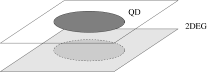
FIG. 3.: QD - 2DEG.

Our objective is to analyze spectral and parametric correlations through the tunneling current statistics. As before, the bias voltage $V$ and the parallel magnetic field ${\bf B}_{\parallel}$ will be used to identify different contributions to the current-current correlator, and to detect their dependence. In addition to these control parameters, we will employ a perpendicular magnetic field $B_{\perp}$ to probe parametric correlations.

In the finite size setup under consideration, Coulomb charging effects are likely to play some role. For didactical reasons, we will begin by discussing the idealized noninteracting situation in Sec. IV A. Coulomb corrections will then be considered in Sec. IV B where it will be argued that the impact of interactions on the current fluctuations sensitively depends on the parameter regime under consideration.

A Noninteracting case

We are interested in the behavior of a chaotic quantum dot on time scales, where the electron dynamics is ergodic – a ‘zero-dimensional’ system in the standard terminology of mesoscopic physics. For a diffusive system, the time it takes to establish ergodic dynamics is set by $E_{\rm Th}^{-1}$. For nearly clean quantum dots, the ergodicity time depends on the specifics of the boundary scattering potential. Ergodic mesoscopic systems are tailor made to modeling in terms of random matrix theory (RMT). For simplicity, we shall assume that the perpendicular magnetic field is strong enough to globally break time reversal invariance. On the other hand, the field is assumed to be too weak to significantly affect the ballistic dynamics of the charge carriers: $R_{c}\gg{\rm\,min}(L,l)$. Under these conditions, the quantum dot can be modeled in terms of random matrices drawn from the Gaussian Unitary Ensemble (GUE). Specifically, we will describe the upper system in terms of some $N$-dimensional Hermitian matrix Hamiltonian $(H+i\Phi)_{\mu\nu}$, where $H$ is taken from a GUE and the antisymmetric matrix $\Phi$ represents the magnetic field in a way to be discussed momentarily. The indices $\mu,\nu$ can, roughly, be interpreted as discretized spatial coordinates. (Neither the discretization in terms of $N$ sites nor the specific interpretation of the indices will play any role throughout.)

Within the RMT description, space-type matrix elements will be represented as $L^{2}A({\bf x},{\bf x}^{\prime})\to NA_{\mu\nu}$ and the integration over the coordinates of the upper system becomes a matrix trace, $L^{-2}\int d^{2}x\to N^{-1}\sum_{\mu}$. On the other hand, the dynamics in the 2DEG spectrometer underneath is integrable-ballistic implying that, as before, it has to be described in terms of the microscopic Hamiltonian of the two-dimensional electron gas. This type of hybrid modeling, involving RMT in combination with a microscopic Hamiltonian, does not pose any conceptual problems. In our basic formulas, (11), (19), and (23), we describe quantities assigned to the upper system through their RMT representations whereas the correlation functions of the lower system are given by the ballistic expression (24). Specifically, the RMT representation of the correlation function $F^{[D]}$ of the upper systems is given by

$$F_{1}^{[D]}({\bf x},{\bf x}^{\prime})\to F_{1\mu\nu}^{[D]}\equiv\langle G_{1\mu\nu}^{-}G_{1\nu\mu}^{+}\rangle,$$

where $G_{\mu\nu}^{\pm}=(\epsilon\pm i0-H\mp i\Phi/2)^{-1}_{\mu\nu}$ are the RMT Green functions, and we have assumed that the mean value of the perpendicular field $B_{\perp}^{+}$ has been absorbed into the Hamiltonian $H$. The other two correlation functions $F^{[d;C]}$ are given by similar expressions with exchanged coordinates. Notice that none of the functions $F$ actually depends on the coordinate arguments – the ergodic zero-dimensional nature of the dot – which is why no conflicts arise from the simultaneous appearance of RMT and truly space dependent correlation functions in Eq. (19).

To be specific, let us assume – a condition easily met experimentally – that the electron dynamics on scales $L$ is ballistic. The average tunneling conductance between the dot and the extended system is again given by Eq. (7). The only difference is that, for a clean quantum dot with irregular boundary scattering, the scale $\Gamma$ is given by $\Gamma^{\rm(b)}\sim v_{\rm F}/L$ [where the superscript ‘(b)’ stands for ballistic].

Turning to the fluctuations of the conductance, we first note that for a GUE Hamiltonian, the cooperonic correlation function $F^{[C]}=0$, and we are left with $F^{[d;D]}_{1\mu\nu}\equiv F^{[d;D]}$, where the second denotation emphasizes the coordinate independence. Substituting these expressions into Eq. (19), temporarily setting the parallel magnetic field to zero, and integrating over coordinates we obtain

$$C_{G}(V,\Delta B)=2\left(\frac{\Gamma^{\rm(b)}}{\epsilon_{\rm F}}\right)^{2}\left(\Re[F^{[d]}]+\frac{\delta}{2\pi\Gamma^{\rm(b)}}\Re[F^{[D]}]\right)\,.$$ (29)

The global suppression factor $(\Gamma^{\rm(b)}/\epsilon_{\rm F})^{2}\sim(k_{\rm F}L)^{-2}$ stems from the fact that an averaging over the area of the QD is intrinsic to the setup. The further suppression factor $\delta/\Gamma^{\rm(b)}\sim(k_{\rm F}L)^{-1}$ multiplying the diffuson contribution results from the integration over the Green functions of the lower 2DEG. Unlike the density-density contribution, $F^{[D]}$ is weighted by Green functions taken at different coordinates. Integration over these arguments leads to the $k_{\rm F}$-dependent suppression.

According to Eq. (29), the fluctuations of the tunneling conductance are linearly related to the sum of two ergodic correlation functions $F^{[d]}$ and – multiplied by a small constant – $F^{[D]}$. We next turn to the discussion of these objects. RMT parametric correlation functions have been calculated within the framework of the nonlinear sigma model [11, 41]. For completeness we have included a brief review of these analyses in the Appendix. The result, an integral representation of the two functions $F^{[d;D]}$, is given by

$$F^{[d]}(s;b) = \frac{1}{2b}\int\limits_{0}^{\infty}\frac{dy}{y}\,e^{is^{+}y}\,\big{[}e^{-by|y-2|}-e^{-by(y+2)}\big{]}\,,$$ (31)

$$F^{[D]}(s;b) = \frac{1}{2b^{2}}\int\limits_{0}^{\infty}\frac{dy}{y^{3}}\,e^{is^{+}y}\,\big{[}(by|y-2|+1)\,e^{-by|y-2|}$$ (33)

$$\qquad\qquad-(by(y+2)+1)\,e^{-by(y+2)}\big{]}\,.$$

In these equations, the correlation functions are characterized through two dimensionless parameters, $s$ and $b$. The parameter

$$s^{+}=\pi(V-V^{\prime}+i0)/\delta_{\uparrow}$$

measures the energetic mismatch between the two Green functions. (Throughout this section we will add to parameters of the upper/lower system a superscript $\uparrow/\downarrow$, if necessary.) The other parameter, $b\sim(N\delta_{\uparrow})^{-2}{\,\rm tr\,}(\Phi^{2})$, describes the field difference. As shown in Ref. [11], this parameter can unambiguously be related to the magnetic field threading the dot. Comparison of the RMT $\sigma$-model and its microscopic counterpart leads to the identification,

$$2b=\pi^{2}C\phi^{2}\,,$$

where $C=\delta_{\uparrow}^{-2}\langle(\frac{\partial\epsilon_{n}}{\partial\phi})^{2}\rangle$ describes the sensitivity of levels to the applied field, and $\phi=\Delta B_{\perp}L^{2}$ the magnetic flux threading the dot. For a disordered system, $C$ is proportional to the conductance $g$.

For general parameter configurations $(s,b)$, the integrals in Eqs. (31) and (33) cannot be done in closed form. In a number of relevant limiting cases, however, simplifications are possible. We first note that for zero magnetic field difference, $\Delta B_{\perp}=0$, the density-density correlator $F^{[d]}(s,b=0)$ is related to the two-level correlation function (see, e.g., Ref. [42])

$$R_{2}^{u}(s)=-\left({\sin s\over s}\right)^{2}$$

through $\Re F^{[d]}=\pi\delta(s)-R_{2}^{u}(s)$ (the index ‘$u$’ standing for unitary). Thus, the density-density contribution to the current correlation function $C_{I}$ is simply proportional to the level number variance $\Sigma_{2}^{u}(V/\delta_{\uparrow})$. Similarly, the real part of the zero-field diffuson correlation function is given by $\Re F^{[D]}(s,b=0)=\pi\delta(s)$ (where the $\delta$-type dependence on $s$ follows from the condition of particle number conservation)[43]. Notice that the $s=0$ singularity displayed by the two correlation functions is of no relevance for our theory. The reason is that for voltages $\Delta V\sim\delta_{\uparrow}s<\Gamma_{\cal T}$ the tunneling approximation employed in calculating the current is no longer applicable. What happens for smaller voltage differences cannot be figured out within the framework of the present formalism. In principle, the $\sigma$-model description can consistently be extended to include the effect of coherent multiple tunneling. (A treatment neglecting the coherence of higher-order tunneling processes would simply lead to a complex energy shift, $s\to s+i\gamma$, where $\gamma=\pi\Gamma_{\cal T}/\delta_{\uparrow}$ and, very much like dephasing to a smearing of the singular low-energy profile of the correlation functions.) The resulting theory, however, would be significantly more complicated than the present formalism and we will not discuss it any further (thereby paying the price that the very low voltage regime remains out of reach).

We next focus on the dependence of the correlation functions on a magnetic field. There are two different cases to be distinguished: For small field strength, $b\ll 1$, the effect of the magnetic field is essentially nonperturbative (in the sense that the correlation functions are nonanalytic in the inverse field strength $\sim b^{-1}$). In this regime, the conductance correlation function has to be computed through numerical integration of Eqs. (31) and (33). The leading order term for small $b$ is linear in $b$ (i.e., quadratic in the field difference $\Delta B_{\perp}$). For larger fields, $b\gg 1$, a perturbative expansion in powers of $b^{-1}$ and $s^{-1}$ leads to the results

$$F^{[d]}=\frac{1}{(2b-is^{+})^{2}},\qquad F^{[D]}=\frac{2}{2b-is^{+}}$$

which would otherwise obtain from a perturbative diagrammatic analysis (similar to the one outlined in the previous section).

We finally ask how the two contributions $F^{[d]}$ and $F^{[D]}$ contributing to the conductance correlation functions can be distinguished. In general, the factor $(k_{\rm F}L)^{-1}\ll 1$ leads to a massive suppression of the diffuson contribution as compared to the density-density contribution. Since corrections of ${\cal O}((k_{\rm F}L)^{-1})$ have been neglected in applying random matrix theory, anyway, an additional parameter is necessary to resolve the diffuson contribution. As discussed previously within the context of two extended systems, this is exactly what an in-plane magnetic field does: Coupling only to the $D$-contribution, an in-plane field difference ${\bf B}_{\parallel}^{-}={\bf B}_{\parallel}-{\bf B}_{\parallel}^{\prime}$ can be used to selectively identify the $F^{[D]}$ correlation function. In fact, for finite ${\bf B}_{\parallel}^{-}$, the tunneling matrix elements pick up a phase factor that modifies the subsequent integration over the Green functions of the 2DEG. For small fields, this leads to

$$C_{G}(V,\Delta B_{\perp};\Delta{\bf q})-C_{G}(V,\Delta B_{\perp};0)\sim$$

$$\sim -\frac{c_{g}}{(k_{\rm F}L)^{3}}(|\Delta{\bf q}|L)^{2}\,F^{[D]}(s,b)+{\cal O}\left((|\Delta{\bf q}|L)^{4}\right)\,,$$

where $c_{g}$ is a constant of order unity.

The relevant field scale is one flux quantum through the area spanned by the linear size of the QD, $L$, and the distance between the layers, $d$, i.e. $B_{\parallel}^{\rm c}\sim 1/(dL)$. This field scale is typically much larger than the characteristic scale of the perpendicular magnetic field $B_{\perp}^{\rm c}\sim 1/(\sqrt{g}L^{2})$.

Before leaving this section, let us briefly comment on the connection between the present analysis and previous experimental work by Sivan et al. [10]. As mentioned in the introduction, Ref. [10] investigated a setup dot/dot, where the second dot was very small, with extreme level quantization. (That is, in Ref. [10], the role of our 2DEG is assumed by a single quantized level of an ultrasmall device.) Arguing semiquantitatively, Sivan et al. related the statistics of the tunneling conductance to density-density-type parametric correlation functions. Indeed, the experimental data turned out to be in good accord with the RMT prediction, Eq. (31), discussed above. There are two differences to the presently discussed setup: first, the fact that in our system a 2DEG is used as a spectrometer implies that the second, diffuson-type correlation function plays a more important role than in Ref. [10]. (In fact, this type of correlation function should contribute to the data of Ref. [10], too. Due to the fact, that the current flows into a single level, however, this contribution is minute and can safely be neglected.) Second, one may hope that the spatial averaging involved in our formalism leads to a far-reaching elimination of all non-spectral structures (as opposed to single-level spectroscopy, where non-universal wave function characteristics may affect the result). The price one has to pay is the suppression factor $(k_{\rm F}L)^{-2}$ that is not present in the dot/dot setup.

Summarizing, we have found that the statistics of the dot/2DEG-conductance (in a regime of broken time reversal invariance) can be described in terms of two basic correlation functions $F^{[d]}$ and $F^{[D]}$. As compared to the previously discussed case of two extended systems, the information contained in $F^{[d;D]}$ is now purely spectral. (All spatial structures have equilibrated due to the ergodicity of the system.) Indeed, these two functions are fully universal in the sense that they depend only on the two basic parameters $s$ and $b$ measuring bias voltage and perpendicular magnetic field strength, respectively. There is one non-universal element affecting the conductance fluctuations, viz., a geometry-dependent factor suppressing the contribution of $F^{[D]}$. Still the contributions of the $d$- and $D$-correlation function can be disentangled, namely, by measuring the dependence of the conductance on a parallel magnetic field. These results have been obtained within a noninteracting theory. We next ask what might change once Coulomb interactions are switched on.

B Coulomb interaction effects

As far as quantum dots are concerned, the most important manifestation of interaction phenomena is the Coulomb blockade: due to the repulsive interaction, it costs extra energy $E_{c}$ to add an electron to the dot. For an isolated dot, this charging energy is determined through the self-capacitance $C$ through $E_{c}=e^{2}/(2C)$. However, for a dot in close vicinity to an extended conducting system, a 2DEG, say, an excess charge on the dot will be compensated for by the accumulation of positive background charge in the large system. Under such circumstances it is the geometric capacitance between the systems that determines the charging energy. This is the situation given presently.

For a planar dot/2DEG setup, the geometric capacitance estimates to $C=\epsilon\epsilon_{0}L^{2}/d$ where $\epsilon_{0}\approx 8.9\cdot 10^{-12}$ F$/$m and $\epsilon$ is the dielectric constant of the filling medium. For GaAs, $\epsilon\approx 10$. The capacitance determines the charging energy $E_{c}$ that has to be compared with the other characteristic energy scales of the problem. The smallest scale we might hope to resolve is the single-particle-level spacing $\delta_{\uparrow}$ of the dot. (It is this energy scale on which non-perturbative structures in the parametric correlation functions are observed.) Notice that both, $\delta_{\uparrow}=(\nu L^{2})^{-1}$ and $E_{c}$, scale inversely with the dot area. Thus, it must be the spacing between dot and 2DEG that determines the crossover criterion. Specifically, with $\nu\approx 3\cdot 10^{10}$ ${\rm meV}^{-1}{\rm cm}^{-2}$, we find that $E_{c}\approx\delta_{\uparrow}$ for $d\approx 4$ nm. Realistically, $d$ is somewhat larger than that, i.e., of the order of up to a few tens of nanometers. We thus conclude that interaction effects are of relevance once one gets interested in low-energy structures of the order of the level spacing.

In previous sections, we have described fluctuations of tunneling transport coefficients through disorder correlation functions ${\cal F}_{0}(\epsilon_{1}-\epsilon_{2})\equiv\langle A_{0}(\epsilon_{1})A_{0}(\epsilon_{2})\rangle$, where $A_{0}(\epsilon)$ are the energy-dependent spectral functions and the subscript ‘$0$’ means ‘noninteracting’. (In fact, we have largely focused on the correlator of Green functions $F_{0}\sim\langle G_{0}^{-}G_{0}^{+}\rangle$. Presently, however, it will be more convenient to concentrate on the spectral functions themselves. The two quantities $F_{0}$ and ${\cal F}_{0}$ are related through ${\cal F}_{0}=\langle A_{0}A_{0}\rangle_{c}=2\Re\langle G_{0}^{-}G_{0}^{+}\rangle_{c}=2\Re F_{0}$.) As mentioned above, interactions will mainly manifest themselves through global charging mechanisms. This sector of the Coulomb interaction does not couple to the coordinate dependence of the correlation functions. To simplify the notation, we therefore temporarily suppress spatial coordinates in the notation.

Our main goal will be to show that interaction and disorder are largely separable in the analysis of correlation functions. Yet, unlike in the noninteracting case, it will no longer be sufficient to compute the zero-temperature correlation functions and to account for finite temperature effects in the end, through an integration over the Fermi distribution functions. Instead, we have to work in a finite-temperature formalism from the outset.

To model the interaction we employ the ‘orthodox model’, that is we add a charging term

$$H_{c}=\frac{e^{2}}{2C}(\hat{N}_{QD}-\bar{N})^{2}\,,$$ (34)

to the Hamiltonian of the dot. Here $\bar{N}$ is the preferred occupation number that can be set by the gate voltage.

To incorporate this term into the model, it is convenient to switch to a functional integral formulation. Within this approach, it is straightforward to see that the theory essentially splits into two sectors: one that describes noninteracting Green functions (albeit subject to some imaginary time dependent voltage $\sigma$), and an interaction- and temperature-dependent weight function that controls the fluctuations of $\sigma$. This approach of describing charging was introduced by Kamenev and Gefen [44]. In the following, we shall briefly review its main elements, and apply it to our present problem.

Within a fermion field integral approach, the imaginary time action describing the quantum dot is given by

$$S=\int d\tau\bar{\psi}(\partial_{\tau}+H_{0}-\mu)\psi+E_{c}\int d\tau(\bar{\psi}\psi-\bar{N})^{2},$$

where $\psi$ is a time- and position-dependent Grassmann field and the rest of the notation is self explanatory. (Unless stated otherwise, the notation $\bar{\psi}\psi\equiv\int d^{2}r\bar{\psi}({\bf r})\psi({\bf r})$ contains a spatial integration.) Decoupling, the interaction by a Hubbard-Stratonovich transformation one obtains the effective action

$$S[\psi,\sigma] = S[\sigma]+S_{\rm d}[\psi,\sigma],$$

$$S[\sigma]=\int d\tau(\frac{1}{4E_{c}}\sigma^{2}-i\bar{N}\sigma),$$

$$S_{\rm d}[\psi,\sigma]=\int d\tau\bar{\psi}(\tau)\left(\partial_{\tau}+H-\mu+i\sigma\right)\psi(\tau),$$

where $\sigma(\tau)$ is a scalar bosonic field. Next, all but the static component $\sigma_{0}\equiv\beta\int d\tau\,\sigma$ are removed from the fermionic action, $S_{\rm d}$, through the gauge transformation $\psi(\tau)\to\exp[-\int^{\tau}d\tau^{\prime}(\sigma(\tau^{\prime})-\sigma_{0})]\psi(\tau)$. [That the static component cannot be removed has to do with the fact that gauging out $\sigma_{0}$ would, in general, lead to a violation of the time-antiperiodic boundary condition $\psi(\tau)=-\psi(\tau+\beta)$.] This makes the action of the system insensitive to the time-dependent components of the Coulomb field. However, the (imaginary time) Green functions ${\cal G}(\tau)$, we actually wish to compute, being non-gauge invariant objects, pick up a gauge factor ${\cal G}(\tau,\sigma)\to{\cal G}(\tau,\sigma_{0})B(\tau)$ to be specified momentarily. For temperatures larger than the level spacing, the integration over the static component $\sigma_{0}$ can be done in a saddle point approximation. As a result, ${\cal G}(\tau,\sigma_{0})\to{\cal G}_{0}(\tau,\bar{\mu})\equiv{\cal G}_{0}(\tau)$, where $\bar{\mu}$ has the significance of an effective (real) chemical potential determined through the optimal occupation number $\bar{N}$.

We are thus led to consider the combination ${\cal G}(\tau)={\cal G}_{0}(\tau)B(\tau)$. Roughly speaking, the physics of interactions resides in the factor $B(\tau)$. Disorder, the external fields, etc., are contained in ${\cal G}_{0}={\cal G}_{0}({\bf x},{\bf x}^{\prime};\tau)$. This is the ‘splitting’ of the zero-mode interaction theory into two components mentioned above.

Transformation of ${\cal G}$ back to frequency space obtains [44]

$${\cal G}(i\epsilon_{n}) = -\frac{1}{2}\int\frac{d\omega^{\prime}}{2\pi}\frac{d\epsilon^{\prime}}{2\pi}B(\omega^{\prime})A_{0}(\epsilon^{\prime})\times$$ (36)

$$\times\frac{\coth\frac{\omega^{\prime}}{2T}+\tanh\frac{\epsilon^{\prime}}{2T}}{i\epsilon_{n}-\omega^{\prime}-\epsilon^{\prime}}\,,$$

where $A_{0}$ is the spectral function associated with the (real-time) Green function $G_{0}$ and

$$B(\omega)=2\sqrt{\frac{\pi}{TE_{c}}}\exp[-\frac{1}{4TE_{c}}(E_{c}^{2}+\omega^{2})]\sinh\frac{\omega}{2T}.$$

This representation holds for any particular realization of the disorder and the external fields.

We next turn to the discussion of the correlator of two spectral functions ${\cal F}(\omega;\epsilon)\equiv\langle A(\epsilon+\frac{\omega}{2})A(\epsilon-\frac{\omega}{2})\rangle$. Making use of Eq. (36) and noticing that the disorder average couples only to the functions $A_{0}$, we obtain

$${\cal F}(\omega;\epsilon) = \frac{\pi}{TE_{c}}\,e^{-\frac{E_{c}}{2T}}\int\frac{d\eta}{2\pi}\,{\cal F}_{0}(\omega-\eta)\,e^{-\frac{\eta^{2}}{8TE_{c}}}\times$$ (38)

$$\times\int\frac{dW}{2\pi}e^{-\frac{W^{2}}{2TE_{c}}}\frac{\cosh\frac{\epsilon}{T}+\cosh\frac{\omega}{2T}}{\cosh\frac{\epsilon\!-\!W}{T}+\cosh\frac{\omega\!-\!\eta}{2T}}\,.$$

Notice that, unlike ${\cal F}$, the non-interacting ${\cal F}_{0}$ depends only on the energy difference $\omega$.

Equation (38) represents the most general form of our result for the correlation function in the presence of a charging interaction. To understand the structure of this expression, and to identify physically distinct regimes, we realize that ${\cal F}$ depends on four characteristic energy scales: the temperature $T$, the charging energy $E_{c}$, the bias voltage $V$, and an intrinsic scale $\epsilon_{0}$ over which the non-interacting correlator ${\cal F}_{0}$ varies. Notice that the dependence on $V$ is implicit, through the limits imposed on the variables $\epsilon$ and $\omega$.

To exemplify the dependence of the correlator on these scales, let us assume that ${\cal F}_{0}(\omega)$ is proportional to a delta function smeared over the intrinsic level broadening $\Gamma_{\cal T}$, i.e., ${\cal F}_{0}(\omega)\sim\delta_{\Gamma_{\cal T}}(\omega)$ (as is the case, e.g., for the diffuson-contribution to the ergodic correlation functions discussed above). In this limit,

$${\cal F}^{(\delta)}(\omega;\epsilon) \sim \frac{1}{2\sqrt{TE_{c}}}e^{-\frac{\omega^{2}}{8TE_{c}}}f(\epsilon)\,,$$ (39)

where $f$ is some function that decays on a scale set by $T$. This expression displays a feature common to all correlation functions ${\cal F}$ affected by charging: Formerly sharp energy dependences are broadened to Gaussians of width $\sigma=2\sqrt{TE_{c}}$. In other words, energetically sharp features of ${\cal F}_{0}$ are washed out and a lower limit to what can be resolved in an experiment is set.

To make further progress, we have to distinguish between two different regimes: (a) weak interaction or high temperature, $E_{c}\ll T$ and (b) strong interaction or low temperature, $E_{c}\gg T$. We begin by discussing the first case, (a).

For $E_{c}\ll T$, interaction corrections are small and an expansion to first order in the parameter $E_{c}/T$ obtains

$${\cal F}(\omega;\epsilon) = \bar{\cal F}_{0}(\omega)\left(1+{\cal O}(E_{c}/T)\right)\,,$$

where $\bar{\cal F}_{0}$ stands for an energy average of the noninteracting correlator ${\cal F}_{0}$, over a scale $2\sqrt{TE_{c}}$ (as in Eq. (39)). This means that weak interactions leave the result essentially unaltered, albeit lowering its spectral resolution.

We next turn to the discussion of case (b), $E_{c}\gg T$. Given that the principal setup of the theory favors low temperatures, this regime is more relevant than (a). On the other hand, it also has to be kept in mind that the applicability of the theory [44] is limited to temperatures $T>\delta$. Thus, the structures discussed below apply to a temperature regime $\delta<T\ll E_{c}$.

In the extreme limit $T\to 0$ [45], the interactions produce a hard Coulomb gap, i.e. ${\cal F}={\cal F}_{0}\,\theta(\epsilon-|\omega|/2-E_{c})$. At finite temperatures the gap becomes softer but its essential features remain robust: For small bias $V$, the correlation function is strongly suppressed while at large bias there are only small changes. The relevant limits are (b1) $V\ll T\sqrt{E_{c}/T}$ and (b2) $T\ll E_{c}\ll V$.

In the first case, when the applied voltage is small, Eq. (38) simplifies to

$${\cal F}(\omega;\epsilon) \simeq c\,\bar{\cal F}_{0}(0)e^{-\frac{E_{c}}{2T}}(\cosh\frac{\epsilon}{T}+\cosh\frac{\omega}{2T}),$$

i.e., the correlator is exponentially suppressed. Here $c$ is a factor depending algebraically on $T/E_{c}$.

In the opposite case, when the applied voltage is large, one obtains

$${\cal F}(\omega;\epsilon) \simeq \bar{\cal F}_{0}(\omega)-$$

$$-e^{-\frac{\epsilon-2E_{c}}{T}}\big{(}\bar{\cal F}_{0}(\omega-)\,e^{-\frac{\omega}{2T}}+\bar{\cal F}_{0}(\omega+)\,e^{\frac{\omega}{2T}}\big{)}\,,$$

where the dominant contribution $\bar{\cal F}_{0}(\omega)$ is the noninteracting ${\cal F}_{0}$ smeared out over energies $2\sqrt{TE_{c}}$ as before and $\omega\pm=\omega\pm 2E_{c}$.

Summarizing, large charging energies, $E_{c}>T$, change the noninteracting theory in two different ways. First, to avoid the Coulomb blockade, large bias voltages $V>E_{c}$ have to be applied. Second, even for those voltages, a lower limit $2\sqrt{TE_{c}}$ on the maximal energetic resolution of the theory is imposed. For the reasons outlined above, we believe that, at least for sufficiently weak magnetic fields and impure samples, the effect of other interaction mechanisms is relatively minor. At any rate, since the functional dependence of the Coulomb blockade corrections follows from Eq. (38), the applicability of the theory can be put to test.

V Conclusions

In this paper, we have introduced an approach to exploring the three basic two-particle correlation functions of mesoscopic physics, the generalized diffuson $F^{[D]}$, the cooperon $F^{[C]}$, and the density-density correlator $F^{[d]}$. The basic idea is to monitor the current flowing between two parallel 2DEGs as a function of three qualitatively different control parameters – a parallel magnetic field, a perpendicular field, and a bias voltage.

As compared to standard transport measurement architectures, the most important advantage of the approach is that electronic correlations are detected without disturbing the ‘bulk’ system through local contacts. Instead the entire planar electron system acts as an ‘extended contact’ whose spatial structure is, nondisturbingly, scanned by means of the two magnetic fields; spectral electronic structures are resolved by measuring the bias voltage dependence of the current. Importantly, the relevant information carried by the tunneling current is solely contained in its fluctuations. For example, we have shown that the Fourier transform of the current-current correlation function with respect to the external field, directly obtains the two spatially resolved transport functions $F^{[D;C]}$. In contrast, previous analyses of magnetotunneling currents, both experimentally and theoretically, focused on the average current profile that is unrelated to any ‘mesoscopic’ type of information.

To exemplify the usefulness of the approach, we have considered two different applications: tunneling between two extended 2DEGs and tunneling from a quantum dot geometry into a 2DEG. As for the former, we have shown how, at least in principle, the exponents characterizing localization/delocalization transitions can be extracted from the current data. In contrast, for a quantum dot with ergodic dynamics, the focus is on spectral rather than on spatial structures. We have explicitly worked out the connection between the tunneling current statistics and various parametric correlation functions (a connection previously used on a semiquantitative basis to interpret the data of the experimentreported in Ref. [10]) and discussed how these correlations can be monitored by changing external field and bias voltage.

As with any other tunneling setup, Coulomb interactions are likely to change the outcome of the noninteracting theory. We have provided evidence in favor of the Coulomb blockade being the most relevant interaction mechanism. The presence of the Coulomb blockade will result in two principal effects: first, it forces one to use bias voltages in excess of the blockade threshold. Second, the spectral structure of the correlation functions is washed out. This reduces the information content that can be extracted from the tunneling current statistics. The extent to which these obstructive mechanisms affect the theory is set by the Coulomb charging energy. In the present system, the latter is largely determined by the inverse of the interlayer capacitance which, owing to the extended geometry of the systems, is small. Thus, charging phenomena will be less pronounced than in small islands. All in all, we believe that for realistic values of the relevant system parameters, a significant parameter range over which electronic correlations can be resolved through the current approach remains.

Acknowledgments: We are grateful to B.L. Altshuler and L.S. Levitov for valuable discussions. This work was supported by the Deutsche Forschungsgemeinschaft (DFG).

A RMT Correlation Functions

In this appendix, we briefly recapitulate the essential steps of the the nonlinear $\sigma$ model (NL$\sigma$M) analysis of RMT parametric correlation functions. The goal is to compute correlation functions of an advanced and a retarded Green function taken at different energies and magnetic fields. To model the field difference, we assume that the Hamiltonian of the retarded/advanced Green function is given by $H\pm i\Phi/2$. Here $\Phi$ is some antisymmetric matrix that can be modeled in a variety of different ways [46]. We are thus led to consider correlation functions of the type

$$F_{\mu\nu\mu^{\prime}\nu^{\prime}}\equiv\langle(\epsilon^{+}+\frac{\omega}{2}-H-i\Phi/2)^{-1}_{\mu\nu}$$

$$\hskip 85.35826pt(\epsilon^{-}-\frac{\omega}{2}-H+i\Phi/2)^{-1}_{\mu^{\prime}\nu^{\prime}}\rangle.$$

Correlation functions of this type can conveniently be calculated from the functional integral [47]

$$\int{\cal D}[\psi,\bar{\psi}]\,e^{-S[\psi,\bar{\psi}]}(\dots)\,,$$ (A1)

$$\qquad\qquad S=i\bar{\psi}\Lambda^{1/2}\{\epsilon-H-({\omega^{+}\over 2}-i\Phi)\Lambda\}\Lambda^{1/2}\psi\,.$$ (A2)

Here $\Lambda=\sigma_{3}^{\sc ar}$ is a Pauli matrix in the ‘advanced-retarded’ space, $\omega^{+}=\omega+i0$, and the ellipses stand for pre-exponential terms specific to the index configuration of the correlation function under consideration [47, 46]. Following a by now standard procedure [47, 46, 11], the average over the RMT Hamiltonian then leads to the effective action of the NL$\sigma$M,

$$S_{\rm eff}=\frac{s^{+}}{2}\,{\rm STr}(Q\Lambda)-\frac{b}{4}\,{\rm STr}(Q\Lambda)^{2}\,,$$ (A3)

where $Q$ is a four-dimensional supermatrix subject to the constraint $Q^{2}=1$. The parameters, $s$ and $b$, appearing in this expression measure the ‘mismatch’ of our two Green functions. Their relation to system parameters is discussed in Sec. IV A.

At this stage the computation of the parametric correlation functions $F^{[d;D;C]}$ amounts to an integral over the four-dimensional matrix $Q$. The explicit calculation [11, 41] leads to $F^{[C]}=0$ and the two one-dimensional integral representations displayed in Eqs. (31) and (33) in the main text.

REFERENCES

- [1] Mesoscopic Phenomena in Solids, edited by B.L. Altshuler, P.A. Lee, and R.A. Webb (North-Holland, New York, 1991); Mesoscopic Quantum Physics, Les Houches, Summer Session LXI, edited by E. Akkermans, G. Montambaux, J.-L. Pichard, and J. Zinn-Justin (North-Holland, Amsterdam, 1995); Mesoscopic Electron Transport, Vol. 345 of NATO Advanced Study Institute, Series E: Applied Sciences, edited by L.L. Sohn, L.P. Kouwenhoven, and G. Schön (Kluwer, Dordrecht, 1997); B.D. Simons and A. Altland, in Theoretical Physics at the End of the XXth Century, Banff, CRM Series in Mathematical Physics (Springer, New York, 2001).
- [2] C.J. Chen, Introduction to Scanning Tunneling Microscopy (Oxford University Press, New York, 1993).
- [3] J. Smoliner, W. Demmerle, G. Berthold, E. Gornik, G. Weimann, and W. Schlapp, Phys. Rev. Lett. 63, 2116 (1989).
- [4] J.P. Eisenstein, T.J. Gramila, L.N. Pfeiffer, and K.W. West, Phys. Rev. B 44, 6511 (1991).
- [5] A. Altland, C.H.W. Barnes, F.W.J. Hekking, and A.J. Schofield, Phys. Rev. Lett. 83, 1203 (1999).
- [6] Y. Oreg and B.I. Halperin, Phys. Rev. B 60, 5679 (1999).
- [7] C.W.H. Barnes, private communication.
- [8] L. Zheng and A.H. MacDonald, Phys. Rev. B 47, 10619 (1993).
- [9] J.S. Meyer, A. Altland, and M. Janssen, Ann. Phys. (Leipzig) 8, SI-173 (1999).
- [10] U. Sivan, F.P. Milliken, K. Milkove, S. Rishton, Y. Lee, J.M. Hong, V. Boegli, D. Kern, and M. de Franza, Europhys. Lett. 25, 605 (1994).
- [11] B.D. Simons and B.L. Altshuler, Phys. Rev. Lett. 70, 4063 (1993); Phys. Rev. B 48, 5422 (1993).
- [12] L. Zheng and A.H. MacDonald, Phys. Rev. B 48, 8203 (1993).
- [13] A.G. Rojo, J. Phys.: Condens. Matter 11, R31 (1999), and references therein.
- [14] Single Charge Tunneling, edited by H. Grabert, J.M. Martinis, and M.H. Devoret (Plenum Press, New York, 1991).
- [15] M.H. Cohen, L.M. Falicov, and J.C. Phillips, Phys. Rev. Lett. 8, 316 (1962).
- [16] Here, ‘weak’ means that the typical energy scale associated with the tunneling, , is much smaller than the other relevant energy scales. In principle, the effect of higher order tunneling processes can be systematically taken into account. Within an approximation whereby higher-order tunneling is treated as an incoherent process this leads to the level smearing mentioned in the text (see also Sec. IV below.) Due to the assumption, , a more complicated, coherent description is not necessary.
- [17] G.D. Mahan, Many-Particle Physics (Plenum Press, New York, 1981).
- [18] Correlations in the disorder potentials might become important if the impurities were placed between the 2DEGs which, in a usual setup, is not the case. In principle, long-ranged fluctuations of the Coulomb potential due to remote impurity sites may be felt by both layers simultaneously. In practice, however, these potentials are strongly screened by the layers themselves which implies that no significant interlayer correlation remains. Notice that correlation effects become ‘significant’ once the amplitude of the correlated part of the scattering potential parametrically exceeds that of the uncorrelated potential.
- [19] The Quantum Hall Effect, edited by R. Prange, and S. Girvin (Springer, Berlin, 1990).
- [20] S. Girvin, in Topological Aspects of Low Dimensional Systems, Les Houches, Summer Session LXIX, edited by A. Comtet, T. Jolicoeur, and S. Ouvry (Springer, New York, 1999).
- [21] Typically, the relevant time scale for Coulomb drag is much larger than the momentum relaxation within each layer, see, e.g., Ref. [12].
- [22] J.P. Eisenstein, L.N. Pfeiffer, and K.W. West, Phys. Rev. Lett. 74, 1419 (1995).
- [23] N. Turner, J.T. Nicholls, E.H. Linfield, K.M. Brown, G.A.C. Jones, and D.A. Ritchie, Phys. Rev. B 54, 10614 (1996).
- [24] L.S. Levitov, private communication.
- [25] In this paper, the term ‘average’ stands for averages over different realizations of an impurity potential; in practice, averaging will mostly be done over external control parameters, e.g. perpendicular external magnetic fields, the chemical potential, or the system geometry. (For sufficiently strong variations of the control parameter) these different procedures are believed to produce equivalent results.
- [26] Notice that, in contrast to many other transport characteristics of electronic systems, the average tunneling current is related to the mean free path and not the transport mean free path . In systems with small angle scattering events, the latter can exceed by an order of magnitude.
- [27] A.D. Stone, in Physics of Nanostructures, Vol. 38 of Scottish Universities Summer Schools in Physics Series, edited by J.H. Davies and A.R. Long (IOP, Bristol, 1993).
- [28] L.S. Levitov and A.V. Shytov, preprint cond-mat/9510006.
- [29] A.M. Rudin, I.L. Aleiner, and L.I. Glazman, Phys. Rev. B 55, 9322 (1997).
- [30] J. Rollbühler and H. Grabert, preprint cond-mat/0102010.
- [31] I.S. Gradshteyn and I.M. Ryzhik, Table of Integrals, Series, and Products (Academic Press, New York, 1965), p. 998.
- [32] G. Bergmann, Phys. Rep. 107, 1 (1984).
- [33] A. Abrahams, P.W. Anderson, D.C. Licciardello, and T.V. Ramakrishnan, Phys. Rev. Lett. 42 (1979) 673.
- [34] R. Merkt, M. Janssen, and B. Huckestein, Phys. Rev. B 58, 4394 (1998), and references therein.
- [35] M. Janssen, O. Viehweger, U. Fastenrath, and J. Hajdu, Introduction to the Theory of the Integer Quantum Hall Effect (Wiley-VCH, Weinheim, 1994).
- [36] M.P. Sarachik and S.V. Kravchenko, preprint cond-mat/9903292 and references therein.
- [37] J.T. Chalker, Physica A 167, 253 (1990).
- [38] M. Janssen, Phys. Rep. 295, 1 (1998).
- [39] B. Huckestein and M. Backhaus, Phys. Rev. Lett. 82, 5100 (1999).
- [40] A. Wieck, private communication.
- [41] N. Taniguchi and B.L. Altshuler, Phys. Rev. Lett. 71, 4031 (1993); N. Taniguchi, B.D. Simons, and B.L. Altshuler, Phys. Rev. B 53, R7618 (1996).
- [42] T. Guhr, A. Müller-Groeling, and H.A. Weidenmüller, Phys. Reports 299, 189 (1998).
- [43] It is straightforward to generalize the result to the orthogonal case by replacing in by the corresponding function and multiplying the diffuson contribution by a factor of 2 ( at ).
- [44] A. Kamenev and Y. Gefen, Phys. Rev. B 54, 5428 (1996).
- [45] Strictly speaking, the limit is not compatible with the condition , but it yields qualitatively correct results.
- [46] A. Altland, S. Iida, and K.B. Efetov, J. Phys. A 26, 3545 (1993).
- [47] K.B. Efetov, Adv. Phys. 32, 32 (1983); Supersymmetry in Disorder and Chaos (Cambridge University Press, New York, 1997).