The World of the Complex Ginzburg-Landau Equation
Abstract
The cubic complex Ginzburg-Landau equation is one of the most-studied nonlinear equations in the physics community. It describes a vast variety of phenomena from nonlinear waves to second-order phase transitions, from superconductivity, superfluidity and Bose-Einstein condensation to liquid crystals and strings in field theory. Our goal is to give an overview of various phenomena described the complex Ginzburg-Landau equation in one, two and three dimensions from the point of view of condensed matter physicists. Our approach is to study the relevant solutions to get an insight into nonequilibrium phenomena in spatially extended systems.
Contents
toc
I Preliminary Remarks
A The equation
The cubic complex Ginzburg-Landau equation (CGLe) is one of the most-studied nonlinear equations in the physics community. It describes on a qualitative, and often even on a quantitative level a vast variety of phenomena from nonlinear waves to second-order phase transitions, from superconductivity, superfluidity and Bose-Einstein condensation to liquid crystals and strings in field theory (Kuramoto, 1984, Cross and Hohenberg, 1993, Newell et al, 1993, Pismen, 1999, Bohr et al, 1998, Dangelmayr and Kramer, 1998).
Our goal is to give an overview of various phenomena described by the CGLe from the point of view of condensed matter physicists. Our approach is to study the relevant solutions to get insight into nonequilibrium phenomena in spatially extended systems. More elementary and detailed introductions into the concepts underlying the equation can be found in Manneville (1990), van Saarloos (1993), van Hecke et al (1994), Nicolis (1995) and Walgraaf (1997).
The equation is given by
| (1) |
where is a complex function of (scaled) time and space (often in reduced dimension or ) and the real parameters and characterize linear and nonlinear dispersion. The equation arises in physics in particular as a “modulational” (or “envelope” or “amplitude”) equation. It provides a reduced, universal description of “weakly nonlinear” spatio-temporal phenomena in extended (in ) continuous media whose linear dispersion is of a very general type (see below) and which are invariant under a global change of gauge (multiplication of by ). This symmetry typically arises when is the (slowly varying) amplitude of a phenomenon that is periodic in at least one variable (space and/or time) as a consequence of translational invariance of the system.
The assumptions of slow variation and weak nonlinearity are valid in particular near the instability of a homogeneous (in ) basic state and Eq. (1) can be viewed as a (generalized) normal form of the resulting ”primary” bifurcation. Then, in analogy with phase transitions, is often called an order parameter.
To see more clearly the analogy with the order parameter concept we write the equation in the unscaled form, ***except maybe for a simple rescaling and rotation of the coordinate system, see below as derived for example from the underlying set of basic (e.g. hydrodynamic) equations for a definite physical situation
| (2) |
Equation (1) is obtained from (2) by the transformations , , and . The case and was assumed. Otherwise the signs in front of the first and/or last term on the right-hand side of (1) have to be reversed. The physical quantities (temperature, velocities, densities, electric field etc.) are given in the form
| (3) |
(c.c. complex conjugate, h.o.t. higher-order terms). If the phenomena occur in (thin) layers, on surfaces, or in (narrow) channels, then , derived from the linear problem, describes the spatial dependence of the physical quantities in the transverse direction(s). is a linear eigenvector and the corresponding eigenvalues. In the case of periodically driven systems, would include a periodic time dependence.
In order to identify the character of the various terms in the linear part of (2) one may also consider the dispersion relation obtained from (2) and (3) for small harmonic perturbations of the basic state
| (4) |
Here is the wavevector in the physical system and is the complex growth rate of the perturbation. is a characteristic time, is the coherence length, a linear group velocity, and a correction to the Hopf frequency . measures in a dimensionless scale the distance from threshold of the instability, i.e. , with the control parameter that carries the system through the threshold at . Note that there is an arbitrary overall factor in Eqs. (2) and (4) which is fixed by the ultimately arbitrary choice of the definition of . The value of the nonlinear coefficient in Eq. (2) depends on the choice of the normalization of the linear eigenvector .
Now we can proceed to summarize the conditions for validity of the CGLe. The following four points are to some extent interrelated.
a) Correct choice of order parameter space, i.e. a single complex scalar: First of all this necessitates that and/or are nonzero, because otherwise one would expect a real order parameter as in simple phase transitions. An exception is the transition to superconductivity and superfluidity where the order parameter is complex for quantum mechanical reasons (see below). Moreover, if , one may run into problems with conservation laws which frequently exclude a homogeneous change of the system. In this case of long-wavelength instabilities often somewhat different order-parameter equations arise (see e.g. Nepomnyashchii, 1995a). Secondly, a discrete degeneracy (or near degeneracy) of neutral modes is excluded, which may arise by symmetry (see below for an example) or by accident. If the eigenvectors of the different modes are different one would need several order parameters and a set of coupled equations. If the eigenvectors coincide (or nearly coincide), which may happen at (or near) a co-dimension-2 point, one can again use one equation, which would now contain higher space or time derivatives.
b) Validity of the dispersion relation (4): since there is no real contribution linear in and since is a positive quantity the real growth rate has a minimum at . In more than 1D this excludes an important class of systems, namely isotropic ones with like Rayleigh-Bénard convection in simple 2D fluid layers. There one has a continuous degeneracy of neutral linear modes. The neglect of terms of higher order in and in is usually justified near the bifurcation.
c) Symmetries: translation invariance in and . Actually the CGLe incorporates translational invariance with respect to space and/or time on two levels. One is expressed by the global gauge invariance, which in the CGLe can be absorbed in a shift of and/or time . Note that this invariance excludes terms that are quadratic in . The other is expressed by the autonomy of the CGLe (no explicit dependence on space and time). The two invariances reflect the fact that the fast and the slow space and time scales are not coupled in this description. This is an approximation which cannot be overcome by going to higher order in the expansion in terms of amplitude and gradients. The coupling effects are in fact nonanalytic in (“non-adiabatic effects”, see, e.g. Pomeau (1984), Kramer and Zimmermann (1985), Bensimon et al (1988)).
d) Validity of the (lowest-order) weakly nonlinear approximation: we will deal mostly with the case of a supercritical (“forward”, or “normal”) bifurcation where and then higher-order nonlinearities in Eq. (1) can be neglected sufficiently near threshold. If the nonlinear term in Eq. (1) has the opposite sign, which corresponds to a subcritical (“backward” or “inverse”) bifurcation, higher-order nonlinear terms are usually essential. However, even in this case, there exist for sufficiently large values of relevant solutions that bifurcate supercritically, which will be discussed in Sec. VI A 1.
From the linear theory we can now distinguish three classes of primary bifurcations where Eq. (1) arises:
i) : for such stationary periodic instabilities is real, and in fact all the imaginary coefficients (including the group velocity ) vanish. Generically, reflection symmetry is needed (see below). Equation (1) then reduces to the “real” Ginzburg-Landau Equation (GLe)
| (5) |
which one might also call the “Complex Nonlinear Diffusion Equation” in some analogy with the Nonlinear Schroedinger Equation (see below). Examples that display such an instability are Rayleigh-Bénard convection in simple and complex fluids, Taylor-Couette flow, electroconvection in liquid crystals and many others. In more than 1D there is the restriction mentioned under b). Thus in isotropic 2D systems the dispersion relation is changed and the Laplacian in Eq.(5) has to be substituted by a different differential operator. The corresponding equation derived by Newell and Whitehead (1969) and by Segel (1969) was in fact the first amplitude equation that included spatial degrees of freedom. It is applicable only for situations with nearly parallel rolls, which is in isotropic systems an important restriction.
So in more than one dimension the system must be anisotropic, which is the case in particular for convective instabilities in liquid crystals (Kramer and Pesch, 1995), but holds also for Rayleigh-Bénard convection in an inclined layer (Daniels et al, 2000) or in a conducting fluid in the presence of a magnetic field with an axial component (Eltayeb, 1971). Also the Taylor-Couette instability in the small gap limit can be viewed as an anisotropic quasi-2D system. In 2D Eq. (5) was first considered in the context of electrohydrodynamic convection in a planarly aligned nematic liquid crystal layer (Pesch and Kramer, 1986, Bodenschatz et al, 1988a, Kramer and Pesch, 1995, for review see also Buka and Kramer, 1996) The Laplacian in Eq. (2) is obtained after a linear coordinate transformation.
ii) : The prime example for such oscillatory uniform instabilities are oscillatory chemical reactions (see e.g. de Wit, 1999). In lasers (or passive nonlinear optical systems) this type may also arise (Newell and Moloney, 1992). In hydrodynamic systems such instabilities are often suppressed by mass conservation (see, however, Börzsönyi et al, 2000). Isotropy does not cause any problems here and the Laplacian applies directly. In the presence of reflection symmetry the group velocity term in Eq. (2) is absent. The spatial patterns obtained from reflect directly those of the physical system. The imaginary parts proportional to and pertain to linear and nonlinear frequency change (renormalization) of the oscillations, respectively. In most systems the nonlinear frequency change is negative (frequency decreases with amplitude), so that with our choice of signs. Coefficients for the CGLe have been determined e.g. from experiments on the Belousov-Zhabotinsky (BZ) reaction (Hynne et al, 1993, Kramer et al, 1994).
iii) : This oscillatory periodic instability occurs in hydrodynamic and optical systems. The best-studied example is Rayleigh-Bénard convection in binary mixtures, although here the bifurcation is in the accessible parameter range mostly subcritical (Schöpf and Zimmermann, 1990, Lücke et al, 1992). Also, in 2D, the system is isotropic, so that the simple CGLe (2) is not applicable. Other 1D examples are the oscillatory instability in Rayleigh-Bénard convection in low Prandtl number fluids, which in 2D occurs as a secondary instability of stationary rolls. In a 1D geometry with just one longitudinal roll it can be treated as a primary bifurcation (Janiaud et al, 1992). Other examples include the wall instability in rotating Rayleigh-Bénard convection (Tu and Cross, 1992, van Hecke and van Saarloos, 1997, Yuanming and Ecke, 1999) and hydrothermal waves, where the coefficients of the CGLe were determined from experiment (Burguette et al, 1999). In 2D the prime example is the electrohydrodynamic instability in nematic liquid crystals in thin and clean cells (otherwise one has the more common stationary rolls) (Treiber and Kramer, 1998). Actually in such an anisotropic 2D system one is lead to a generalization of Eq. (1) where the term is replaced by a more general bilinear form , see Sec. VI D.
Most of the oscillatory periodic systems just mentioned have reflection symmetry and then one has to allow for the possibility of counter-propagating waves which makes a description in terms of two coupled CGLes necessary (see Cross and Hohenberg, 1993). The degeneracy between left and right traveling waves can be lifted by breaking the reflection symmetry by applying additional fields or an additional flow. In this situation one roll system is favored over the other and, if the effect is strong enough, a single CGLe can be used. Breaking reflection symmetry in stationary periodic instabilities (case i)) the rolls will generically start to travel and one indeed arrives at an oscillatory periodic instability (case iii)). This has been studied experimentally by applying a through flow in thermal convection (Pocheau and Croquette, 1984) or in the Taylor-Couette system (Tsameret and Steinberg, 1994; Babcock, Ahlers, and Cannell, 1991) or by non-symmetric surface alignment in electroconvection of nematics (pretilt or hybrid alignment, see e.g. Krekhov and Kramer, 1996).
Since the drift introduces a frequency, for sufficiently strongly broken reflection symmetry the distinction between cases i) and iii) is lost, as is obvious in open-flow systems (Leweke and Provansal, 1994, 1995; Roussopoulos and Monkewitz, 1996).
The CGLe may also be viewed as a dissipative extension of the conservative nonlinear Schrödinger equation (NLSe)
| (6) |
which describes weakly nonlinear wave phenomena (Newell, 1974). The prime examples are waves on deep water, (Dias and Kharif, 1999) and nonlinear optics (Newell and Moloney, 1992). The conservative limit of Eq. (1) is obtained by letting in Eq. (2) with remaining nonzero, so that , and rescaling space and the amplitude.
B Historical remarks
Four key concepts come together in the CGLe philosophy:
-
Weak nonlinearity, which amounts to an expansion in terms of the order parameter . This concept goes back to Landau’s theory of second-order phase transitions (Landau, 1937a). Landau also employed this type of expansion in his attempt to explain the transition to turbulence (Landau, 1944). In the context of stationary, pattern-forming, hydrodynamic instabilities the weakly nonlinear expansion leading to a solvability condition at third order was introduced by Gorkov (1957) and Malkus and Veronis (1958). One should also mention the work of Abrikosov in 1957 (for review see Abrikosov (1988)) where he presents the theory of the mixed state of type II superconductors in a magnetic field based on the Ginzburg-Landau theory of superconductivity. The mixed state is a periodic array of flux lines (or vortices) corresponding to topological defects (see below). Abrikosov introduced a weakly nonlinear expansion to describe this state valid near the upper critical field.
-
Slow relaxative time dependence was first used by Landau in the above-mentioned paper on turbulence in 1944. In the context of pattern-forming instabilities it goes back to Stuart (1960).
-
Slow nonrelaxative time dependence with nonlinear frequency renormalization in the complex-amplitude formulation was introduced by Stuart in 1960 using multi-scale analysis. Of course perturbation theory for periodic orbits (in particular conservative Hamiltonian systems) is a classical subject that was treated by Bogoliubov, Krylov and Mitropolskii in 1937 (for review, see Bogoliubov and Mitropolskii, 1961).
-
Slow spatial dependence was included already by Landau (1937b) in the context of -ray scattering by crystals in the neighborhood of the Curie point. However, the concept became known with the success of the (stationary) phenomenological Ginzburg-Landau (GL) theory of superconductivity [Ginzburg and Landau (1950)].
The stationary GL theory for superconductivity has a particular resemblance to the modulational theories of pattern-forming systems because the order parameter is complex, although for a very different reason. Superconductivity being a macroscopic quantum state requires an order parameter that has the symmetries of a wave function. In spite of the different origin one has many analogies. However, in superconductors the time dependence is rendered nonvariational primarily through the coupling to the electric field due to local gauge invariance (see, e.g. Abrikosov, 1988), a mechanism that has no analog in pattern-forming systems.
The time-dependent GL theory for superconductors was presented (phenomenologically) only in 1968 by Schmid, (derived from microscopic theory shortly afterwards by Gorkov and Eliashberg (1968)), when the first modulational theory was derived in the context of Rayleigh-Bénard convection by Newell and Whitehead (1969) and Segel (1969). Eq. (5) with additional noise term has been studied intensively as a model of phase transitions in equilibrium systems, see e.g. Hohenberg and Halperin (1977).
The full CGLe was introduced phenomenologically by Newell and Whitehead (1971). It was derived by Stewartson and Stuart (1971) and DiPrima, Eckhaus and Segel (1971) in the context of the destabilization of plane shear flow, where its applicability is limited by the fact that one deals with a strongly subcritical bifurcation. In the context of chemical systems the CGLe was introduced by Kuramoto and Tsuzuki (1974).
There exists an extended mathematical literature on the CGLe, which we will touch rather little, see e.g. Doering et al (1987, 1988), Levermore and Stark (1997), Doelman (1995), van Harten (1991), Milke and Schneider (1996), Schneider (1994), Melbourne (1998), Milke (1998).
C Simple model – vast variety of effects
Clearly the CGLe (1) may be viewed as a very general normal-form type equation for a large class of bifurcations and nonlinear wave phenomena in spatially extended systems, so a detailed investigation of its properties is well justified. The equation ”interpolates” between the two opposing limits of the conservative NLSe and the purely relaxative GLe. The CGLe world lies between these limits where new phenomena and scenarios arise, like sink and source solutions (spirals in 2D and filaments in 3D), various core and wave instabilities, nonlinear convective versus absolute instability, screening of interaction and competition between sources, various types of spatio-temporal chaos and glassy states.
II General Considerations
In this Section we will study general properties of Eq. (1) relevant in all dimensions.
A Variational case
For the case of it is useful to transform into a ”rotating“ frame . Then Eq. (1) goes over into
| (7) |
Eq. (7) can be obtained by variation of the functional
| (8) |
leading to and
| (9) |
One sees that for all non-infinite the value of decreases, so the functional (8) plays the role of a global Lyapunov functional or generalized free energy ( is bounded from below). The system then relaxes towards local minima of the functional. In particular the stationary solutions of the GLe (b=0) correspond in the more general case to with corresponding stability properties.
In the NLSe limit the functional becomes a Hamiltonian, which is conserved. More generally, the NLSe is obtained from the CGLe by taking the limit without further restrictions. After rescaling one obtains Eq. (6). One sees that the equation comes in two variants, the focusing ( sign) and defocusing (sign) case (the notation comes from nonlinear optics. In 1D it is completely integrable (Zakharov and Shabat, 1971). In the focusing case it has a two-parameter family of “bright” solitons (irrespective of space translations and gauge transformation). In D solutions typically exhibit finite-time singularities (collapse) (Zakharov, 1984, for recent review see Robinson, 1997). In the defocusing case one has in 1D a three-parameter family of ”dark solitons” that connect asymptotically to plane waves and vortices in 2 and 3D. We will here not discuss the equation since there exists a vast literature on it (see e.g. Proceedings of Conference on The Nonlinear Schrödinger Equation,1994). It is useful to treat the CGLe in the limit of large and from the point of view of a perturbed NLSe.
B The amplitude-phase representation
Often it is useful to represent the complex function by its real amplitude and phase in the form . Then Eq. (1) becomes
| (10) | |||||
| (11) |
For this corresponds to a class of reaction-diffusion equations called systems, which are generally of the form
| (12) | |||
| (13) |
Such equations have been studied in the past extensively by applied mathematicians (see Hagan, 1982, and references therein). Clearly, one can combine Eqs. (10) in such a way that the right-hand sides are those of a system.
C Transformations, coherent structures, similarity
The obvious symmetries of the CGLe are time and space translations, spatial reflections and rotation, and global gauge (or phase) symmetry . The transformation leaves the equation invariant so that only a half plane within the parameter space has to be considered.
Other transformations hold only for particular classes of solutions. To see this it is useful to consider the following transformation
| (14) |
leading to
| (15) |
with . Most known solutions are either of the coherent-structure type, where depends only on its first argument (i.e. with properly chosen it is time independent in a moving frame), or are disordered in the sense of spatio-temporal chaos. Coherent structures can be localized or extended. The “outer wavevector” could be absorbed in (then would be replaced by ). It may be useful to introduce when the gradient of the phase of , integrated over the system, is zero (or at least small).
With a little bit of algebra one can now derive a useful similarity transformation that connects coherent structures along the lines in parameter space. Defining
| (16) |
the transformation relations between unprimed and primed quantities can be written as
| (17) | |||||
| (18) | |||||
| (19) |
The relations (18) are independent of the nonlinear part of (1) and therefore survive generalizations. Solutions with remain stationary (for ) and that transformation was given by Hagan, 1982. Clearly one can very generally transform to , where the CGLe represents a system. Note that for one cannot have and . The similarity line (vanishing group velocity, see below) includes the real case.
Note, that the stability limits of coherent states are in general not expected to conform with the similarity transform. By taking in Eqs. (19) the limit , one finds . Then the in the factor can be dropped and changes in can be absorbed in a rescaling of length. The similarity transformation then connects solutions with arbitrary velocity, which is a manifestation of a type of Galilean invariance (van Saarloos and Hohenberg, 1992). Thus in this limit solutions appear as continuous families moving at arbitrary velocity.
Similarly, by letting , tends to a constant. Then, in addition to the in the factor , the linear growth term can be dropped, and then changes in can be absorbed in a rescaling of B as well as length and time. The similarity transformation then turns into a scaling transformation. Thus in this limit solutions appear as continuous families of rescaled functions.
For and one has both transformations together, so solutions appear generically as two-parameter families. Indeed, one is then left with the NLSe.
D Plane-wave solutions and their stability
The simplest coherent structures are the plane-wave solutions
| (20) |
( is an arbitrary constant phase) which exist for . To test their stability one considers the complex growth rate of the modulational modes. One seeks the perturbed solution in the form
| (21) |
where is a modulation wave vector and are the amplitudes of the small perturbations. One easily finds the expression for the growth rate (Stuart and DiPrima, 1980):
| (22) | |||||
| (23) |
By expanding this equation for small one finds
| (24) |
with
| (25) | |||||
| (26) | |||||
| (27) | |||||
| (28) |
where is the component of parallel to . The quantities and for will be denoted by and . Similarly, for we may use the notation and . Clearly the longitudinal perturbations with are the most dangerous ones. The solutions (20) are long-wave stable as long as the phase diffusion constant is positive. Thus one has a stable range of wave vectors with enclosing the homogeneous () state as long as the “Benjamin-Feir-Newell criterion” holds. This criterion conforms with the similarity transform (19). The condition is the (generalized) Eckhaus criterion. For it reduces to the classical Eckhaus criterion for stationary bifurcations. We will call the quadrants in the plane with the “defocusing quadrants”. Otherwise we will speak of the “focusing quadrants”.
From Eqs. (22,24) one sees that for and the destabilizing modes have a group velocity , so the Eckhaus instability then is of convective nature and does not necessarily lead to destabilization of the pattern (see next subsection).
The Eckhaus instability signalizes bifurcations to quasiperiodic solutions (including the solitary limit), which are of the form (15) with periodic function . It becomes supercritical before the Benjamin-Feir-Newell criterion is reached (Janiaud et al, 1992) and remains so in the unstable range. The bifurcation is captured most easily in the long-wave limit by phase equations, see below. A general analysis of the bifurcating solutions has recently been done (Brusch et al 2000), see subsection III C.
It is well known that the Eckhaus instability in the CGLe is not in all cases of long-wave type. Clearly, a necessary condition for it to be the case is that is positive where changes sign.
From the above expressions one deduces that this fails to be the case for , where
| (30) |
Thus the range is in the defocusing quadrant, far away from the Benjamin-Feir-Newell stability limit. We are presently not aware of effects where this phenomenon is of relevance.
E Absolute versus convective instability of plane waves
For a nonzero group velocity the Eckhaus criterion can be taken only as a test for convective instability. In this case a localized 1D initial perturbation of the asymptotic plane wave, although amplified in time, drifts away and does not necessarily amplify at a fixed position (Landau and Lifshitz, 1959). For absolute instability localized perturbations have to amplify at fixed position. The time evolution of a localized perturbation is in the linear range given by
| (31) |
where is the Fourier transform of . †††It can be shown strictly that the destabilization occurs at first for purely longitudinal perturbations The integral can be deformed into the complex k-plane. In the limit the integral is dominated by the largest saddle point of (steepest descent method, see e.g., Morse and Feshbach, 1953) and the test for absolute instability is
| (32) |
The long-wavelength expansion (24) indicates that at the Eckhaus instability, where becomes negative, the system remains stable in the above sense. When vanishes and the main contribution comes from the term linear in that then can suppress instability.
In the following, results of the analysis are shown in the plane (Aranson et al, 1992; Weber et al, 1992). In Fig. 1 the scenario is demonstrated for four cuts in the space. The stable region (light gray) is limited by the Eckhaus curve, which terminates at on the curve. To the right of it there exists a convectively unstable wavenumber band (dark grey). goes to zero on the Benjamin-Feir-Newell curve as , which can be seen from the long-wavelength expansion (24) with the fourth-order term included. Moving away from the Benjamin-Feir-Newell line (into the unstable regime) increases and decreases until they come together in a saddle-node-type process at a value . Beyond there are no convectively unstable plane waves. The saddle nodes are shown in the plane in Fig. 2 (curve ). Thus, convectively unstable waves exist up to this curve. The Benjamin-Feir-Newell criterion curve up to which convectively unstable waves exist is also included. The other curves include the Eckhaus instability and the absolute stability limit for waves with wavenumber selected by the stationary hole solutions (see Sec. III B).
Eq. (32) by itself gives only a necessary condition for absolute stability. However, it is also sufficient, as long as one of the two roots of the dispersion relation, which collide at the saddle point when is decreased from positive values to zero, say , is the root that produced the convective instability, and if does not cross the real axis before does, when is increased from zero. (Note that has to cross the axis when is increased. Note also that, because of the symmetry one has parallel processes with opposite sign of ). For a discussion of the underlying “pinching condition”, see e.g. Brevdo and Bridges (1996). In the parameter range considered here the sufficient condition is fulfilled.
Clearly the absolute stability boundary can be reached only if reflection at the boundaries of the system is sufficiently weak, so in general one should expect the system to lose stability before the exact limit is reached. In many realistic situations in the CGLe the interaction of the emitted waves with the boundaries leads to sinks (shocks) in analogy to the situation where different waves collide. These shocks are strong perturbations of the plane wave solutions but they absorb the incoming perturbations. Thus here, even for periodic boundary conditions, the absolute stability limit is relevant. Moreover, in infinite systems, states with a cellular structure made up of sources surrounded by sinks can exist in the convectively unstable regime. However, the convectively unstable states are very susceptible to noise, which is exponentially amplified in space. The amplification rate goes to zero at the convective stability limit and diverges at the absolute stability limit.
The concept of absolute stability is relevant in particular for the waves emitted by sources and possibly also for some characteristics of spatio-temporally chaotic states. When boundaries are considered one also has to allow for a linear group velocity term in the CGLe (see Eq. (2)). Such a term does not change the convective stability threshold, but clearly the absolute stability limit is altered, and this is important in particular in the context of open flow systems. The saddle point condition in (32) ensures the existence of bounded solutions of the linear problem that satisfy nonperiodic boundary conditions (irrespective of their precise form) at well separated side walls (sometimes called “global modes”), because for that purpose one needs to superpose neighboring (extended) eigenmodes, which are available precisely at the saddle point. This is an alternative view of the absolute instability (Huerre and Monkowitz, 1990, Tobias and Knobloch, 1998, Tobias, Proctor, and Knobloch, 1998).
Often the condition (32) coincides with the condition that a front invades the unstable state in the upstream direction according to the linear front selection criterion (marginal stability condition, see, e.g. van Saarloos (1988)).
F Collisions of plane waves and effect of localized disturbances
The nonlinear waves discussed above have very different properties from linear waves. In particular, when two waves collide they almost do not interpenetrate. Instead a “shock” (sink) is formed along a point (1D), line (2D), or surface (3D). When the frequency of the two waves differs the shock moves with the average phase velocity, provided there are no phase slips in 1D, or its equivalent in higher dimensions (creation of vortex pairs in 2D and inflation of vortex loops in 3D), for review see Bohr et al (1998). A stationary shock is formed most easily when a wave impinges on an absorbing boundary. Here we will consider the general situation where a plane wave is perturbed by a stationary, localized disturbance. This concept will be particularly useful in the context of interaction of defects.
Sufficiently upstream (i.e. against the group velocity) from the disturbance the perturbation will be small and we can linearize around the plane-wave solution. In general one obtains exponential behavior with exponents calculated from the dispersion relation (22) with . This gives
| (33) |
After separating out the translational mode one is left with a cubic polynomial. To discuss the roots choose the group velocity (otherwise all signs must be reversed). For one has in the Eckhaus stable range. For one finds that increases with increasing . Before is reached and collide and become complex conjugate.
The existence of roots with positive real part is an indication of screening of disturbances in the upstream direction because one needs the solutions that grow exponentially to match to the disturbance. The screening length is given by , the root with the smaller real part. So the screening is in general exponential. The length diverges for and then one has a crossover to power law.
In the focusing quadrants the root collision always occurs before the Eckhaus instability is reached. (It fails to hold only in part of the defocusing quadrant away from the origin and restricted to .) We will refer to the situation where are real to the monotonic case and otherwise to the oscillatory case, because this characterizes the nature of the asymptotic interaction of sources that emit waves, see Sec. III and IV. In Fig. 2 the transition from monotonic to oscillatory behavior for the waves emitted by standing hole solutions is also shown (curve MOH). A generalization to disturbances that move with velocity is straightforward by replacing in Eq. (22) the growth rate by .
G Phase equations
The global phase invariance of the CGLe leads to the fact that, starting from a coherent state (in particular a plane wave), one expects solutions where the free phase becomes a slowly varying function, and one can construct appropriate equations for these solutions. (In the case of localized structures one then also has to allow for a variation of the velocity.) In the mathematical literature these phase equations are sometimes called “modulated modulation equations”. There are several ways to proceed technically in their derivation, but the simplest is to first establish the linear part of the equation by a standard linear analysis and then construct nonlinearities by separate reasoning. It is helpful to include symmetry considerations to exclude terms from the beginning on.
By starting from a plane wave state (20) with wave number in the direction one may perform a gradient expansion of leading in 1D to
| (34) |
Note the absence of a term proportional to which would violate translation invariance. The prefactors of the gradient terms have to be chosen according to (25) in order to reproduce the linear stability properties of the plane wave (with the wavenumber replaced by ).
Nonlinearity can be included in Eq. (34) by substituting in the coefficients of Eq. (25) . Expanding and one generates the leading nonlinear terms, so that eq. (34) goes over into (Janiaud et al, 1992)
| (35) |
with the linear parameters from (25) and
| (36) | |||||
| (37) |
Because of translation invariance the lowest relevant nonlinearities are and [Kuaramoto, 1984].
In the stationary case () one has . The remaining nonlinearity does not saturate the linear instability and one recovers the results for the nonlinear Eckhaus instability (Kramer and Zimmermann, 1985). For and the dominant nonlinearity is which does saturate the linear instability. The resulting equation with
| (38) |
describes the (supercritical) bifurcation at the Benjamin-Feir-Newell instability and is known as the Kuramoto-Sivashinsky equation. It has stationary periodic solutions, which are stable in a small wavenumber range , where (Frisch et al. 1986, Nepomnyashchii, 1995b). It also has spatio-temporally chaotic solutions, which are actually the relevant attractors, and it maybe represents the simplest partial differential equation displaying this phenomenon. Since it is a rather general equation for long-wavelength instabilities, independent of the present context of the CGLe, it has attracted much attention in recent years (see e.g. Bohr et al (1998)).
In the general case both nonlinearities are important (and also the term proportional to ). Then the bifurcation to modulated waves, which are represented by periodic solutions of (34), can be either forward or backward depending on the values of . In fact the Eckhaus bifurcation always becomes supercritical before the Benjamin-Feir-Newell instability is reached. Modulated solutions can be found analytically in the limit , where Eq. (34) reduces to
| (39) |
with . This limit is complementary to that leading to the Kuramoto-Sivashinsky equation and one is in fact left with a perturbed Korteweg de Vries equation. This equation is (in 1D) completely integrable and the perturbed case was studied by Janiaud et al (1992) and by Bar and Nepomnyashchii (1995). They showed that a fairly broad band of the periodic solutions (much larger than in the Kuramoto-Sivashinsky equation equation) persists the perturbation of the Korteweg de Vries equation and is stable. Outside this limit, and in particular in the Kuramoto-Sivashinsky equation regime, one has in extended systems spatio-temporally chaotic solutions. It is believed that this chaotic state is a representation of the phase chaos observed in the CGLe, although this view has been challenged (see Sec. III D). Sakaguchi (1992) introduced higher-order nonlinearities into the Kuramoto-Sivashinsky equation, which allowed to capture the analog of the transition (or cross over) to amplitude chaos manifesting itself by finite-time singularities in .
Under some conditions, namely when is positive and is small, the first nonlinearity in Eq. (35) is dominant and then it reduces to Burgers equation
| (40) |
which is completely integrable within the space of functions that do not cross zero, because it can be linearized by a Hopf-Cole transformation . The equation allows to describe analytically sink solutions (shocks), (see e.g., Kuramoto and Tsuzuki (1976), Malomed (1983) and is (in 2D) useful for the qualitative understanding of the interaction of spiral waves in the limit (see Biktashev (1989), Aranson et al (1991)).
Clearly generalization of the phase equations to higher dimensions is possible. Using the full form of Eq. (25) one can easily generalize the phase equation to 2D (for details see also Kuramoto (1984); Lega (1991)). The equation is most useful in the range where goes through zero and becomes negative. Also, they can be derived outside the range of applicability of the CGLe (far away from threshold) and for more general nonlinear long-wavelength phenomena, where does not represent the phase of a periodic function (see e.g. Bar and Nepomnyashchii (1995)).
H Topological defects
Zeros of the complex field result in singularity of the phase . In 2D point singularities correspond to quantized vortices with so-called topological charge , where is a contour encircling the zero of . Although for they represent wave emitting spirals, they are analogous to vortices in superconductors and superfluids and represent topological defects because a small variation of the field will not eliminate the phase circulation condition. Clearly, vortices with topological charge are topologically stable. The vortices with multiple topological charge can be split into single-charged vortices ‡‡‡In small samples vortices with multiple charge can be dynamically stable, see for detail Geim et al (1998); Deo et al (1997).. 2D point defects become line defects in 3D. Then, one can close such a line to a loop, which can shrink to zero. Some definitions of topological defects from the point of view of energy versus topology are given by Pismen (1999).
Topological arguments do not guarantee the existence of a stable, coherent solution of the field equations. In particular, the stability of the topological defect depends on the background state it is embedded in. For example, spiral waves are stable in a certain parameter range, where they select the background state (see Sec. IV). Simultaneously charged sinks coexist with spirals and play a passive role. Also, defects can become unstable against spontaneous acceleration of their cores.
I Effects of boundaries
Boundaries may play an important role in nonequilibrium systems. Even in large systems the boundary may provide restriction or even selection of the wavenumber. We will not discuss this topic (see, e.g. Cross and Hohenberg, 1993) and consider situations where such effects are not important.
III Dynamics in 1D
In this Section we will consider the properties of various 1D solutions of the CGLe. We will discuss the stability and interaction of coherent structures and the transition to and characterization of spatio-temporal chaos.
A Classification of coherent structures, counting arguments
Coherent structures introduced in the previous chapter can be characterized using simple counting arguments put forward by van Saarloos and Hohenberg (1992). It should be mentioned, however, that the counting arguments cannot account for all the circumstances, for example, hidden symmetries, and may fail for certain class of solutions, see below. 1D coherent structures can be written in the form
| (41) |
with the real functions satisfying a set of 3 ordinary differential equations
| (42) | |||||
| (43) | |||||
| (44) |
Abbreviations used are , and . These ordinary differential equations constitute a dynamical system with three degrees of freedom.
The similarity transform of Sec. II C can be adapted to these equations by absorbing the external wavenumber in the phase , which leads to , , and
| (45) |
The counting arguments allow to establish necessary conditions for the existence of localized coherent structures, which correspond to homo- or heteroclinic orbits of Eqs. (44). Consider, e.g. the trajectory of Eqs. (44) flowing from fixed point to fixed point . If has unstable directions, there are free parameters characterizing the flow on the -dimensional subspace spanned by the unstable eigenvectors. Together with the parameters and this will yield free parameters. If has unstable directions, the requirement that the trajectory should come in orthogonal to these yields conditions. The multiplicity of this type of trajectory will, therefore, be , and, depending on , it will give either a -parameter family (), a discrete set of structures () or no structure (). In addition one may have symmetry arguments that reduce the number of conditions.
The asymptotic states can either correspond to non-zero steady states (plane waves), or to the trivial state . Accordingly, the localized coherent structures can be classified as pulses, fronts, domain boundaries, and homoclons. A pulse corresponds to the homoclinic orbit connecting to the trivial state . They come in discrete sets (Hohenberg and van Saarloos, 1992). For a full description of the pulses see Akhmediev et al (1995,1996,2001), Afanasjev et al (1996). Fronts are heteroclinic orbits connecting on one side to a plane-wave state and to the unstable trivial state on the other side. They come in a continuous family, but sufficiently rapidly decaying initial conditions evolve into a “selected” front that moves at velocity and generates a plane wave with wave number (“linear selection”). For a discussion, see Hohenberg and van Saarloos (1992), Cross and Hohenberg (1993).
Domain boundaries are heteroclinic orbits connecting two different plane-wave states. The domain boundaries can be active (sources, often called holes) or passive (sinks or shocks) depending on whether in the co-moving frame the group velocity is directed outward or inward, respectively. They will be discussed in the next subsection. Homoclons (or homoclinic holes, phasons) connect to the same plane-wave state on both sides. They are embedded in solutions representing periodic arrangements of homoclons, which represent quasiperiodic solutions satisfying ansatz (41) and correspond to closed orbits of Eqs. (44). They will be discussed in Subsec. III C 2. There also exist chaotic solutions of Eqs. (44), which correspond to nonperiodic arrangement of holes and shocks, or homoclons, see Subsecs.III B 2, III C 2.
B Sinks and sources, Nozaki-Bekki hole solutions
Sinks (shocks) conform with the counting arguments of Hohenberg and van Saarloos (1992): there is a two-parameter family of sinks. However, there are no exact analytic expressions for the sink solution connecting two traveling waves with arbitrary wavenumbers. The exact sink solution found by Nozaki and Bekki (1984) corresponds to some special choice of the wavenumbers and is not therefore typical. For small difference in wavenumber a phase description of sinks is possible (Kuramoto, 1984).
However, the counting arguments (which are, strictly speaking, neither necessary nor sufficient, and cannot account for specific circumstances, such as a hidden symmetry) fail for the source solution. According to the counting arguments there should be only a discrete number, including in particular the symmetric standing hole solution that has a zero at the center and emits plane waves of a definite wavenumber (for given ). However, the standing hole is embedded in a continuous family of analytic moving sources, the Nozaki-Bekki hole solutions. They are characterized by a localized dip in that moves with constant speed and emits plane waves with wave numbers .
This is a special feature of the cubic CGLe as demonstrated by the discovery that the moving holes do not survive a generic perturbation of the CGLe, e.g. a small quintic term (see below). Thus they are not structurally stable (Popp et al, 1993, 1995, Stiller et al, 1995a,b). With the perturbation the holes either accelerate or decelerate depending on the sign of the perturbation and other solutions appear, see also Doleman (1995). Clearly, the 1D CGLe possesses a “hidden symmetry” and has retained some remnant of integrability from the NLSe. Apparently this non-genericity has no consequences for other coherent structures.
The Nozaki-Bekki hole solutions are of the form (Nozaki and Bekki, 1984)
| (46) | |||||
| where | (47) |
and , is the velocity of the hole, and are the asymptotic wavenumbers. Symbols with a “hat” denote real constants depending only on and , e.g. . The frequency and are linear functions of . The emitted plane waves have wavenumbers
| (48) |
where and . One easily derives the relation
| (49) |
where is the dispersion relation for the plane waves. This relation can be interpreted as phase conservation and is valid also for more general equations possessing phase invariance. For the cubic CGLe it reduces to , i.e. the hole moves simply with the mean of the group velocities of the asymptotic plane waves. The exact relations between the parameters can be derived by inserting ansatz (46) into the CGLe. The resulting algebraic equations (8 equations for 8 parameters) turn out to be not independent, yielding the one-parameter family. becomes zero at a maximal velocity and here the hole solution merges with a plane wave with wavenumber . In a large part of the plane these bifurcations occur in the range of stable plane waves. This is the case outside a strip around the line given by with varying from for large values of to for small values. The region extends almost to the Benjamin-Feir-Newell curves. The bifurcation cannot be captured by linear perturbation around a plane wave, since the asymptotic wavenumbers of holes differ. Presumably the bifurcation can be captured by the phase equation (35). For only the standing hole survives (the velocities of the moving holes diverge in this limit).
The interest in the hole solutions comes particularly from the fact that they are dynamically stable in some range. The stability has first been investigated by Sakaguchi (1991), in direct simulations of the CGLe. The stability problem was then studied by Chaté and Manneville (1992), numerically for and by Sasa and Iwamoto (1992), semi-analytically for and by Popp et al. (1995), essentially analytically. As a result, hole solutions were found to be stable in a narrow region of the - plane which is shown in Fig. 2 for the standing hole () (upper shaded region). From below, the region is bounded by the border of (absolute) stability of the emitted plane waves with wavenumber (see Eq.(46)) corresponding to the continuous spectrum of the linearized problem, see curve AH in Fig.2. From the other side, the stable range is bounded by the instability of the core with respect to localized eigenmodes corresponding to a discrete spectrum of see curve CI in Fig.2. For , one has
| (50) | |||||
| (51) |
The result could be reproduced fully analytically by perturbing around the NLSe limit, where the Nozaki-Bekki holes emerge as a subclass of the 3-parameter family of dark solitons and is supported by detailed numerical simulations and shows excellent agreement (Stiller et al, 1995a). It differs from that obtained by Lega and Fauve (1997) and by Kapitula and Rubin (2000). Lega and Fauve (1997), Lega (2000) claim a larger stability domain which is in disagreement with simulations (Stiller et al, 1995a).
The core instability turns out to be connected with a stationary bifurcation where the destabilizing mode passes through the neutral mode related to translations of the hole. This degeneracy is specific to the cubic CGLe and is thus structurally unstable (see below). When going through the stability limit the standing hole transforms into a moving one. Indeed, the cores of moving holes were found to be more stable than those of the standing ones (Chatè and Manneville, 1992).
1 Destruction of Nozaki-Bekki holes by small perturbations
Consider the following “perturbed cubic CGLe”
| (52) |
where a quintic term with a small complex prefactor () is included, which will be treated as a perturbation. There are, of course, other corrections to the cubic CGLe, but their “perturbative effect” is expected to be similar.
Simulations with small but finite show that stable, moving holes are in general either accelerated and eventually destroyed or slowed down and stopped to the standing hole solution depending on the phase of (Popp et al 1993, 1995; Stiller et al 1995a,b). In particular, for real one has
| (53) |
One finds that the relations (49) connecting the core velocity and the emitted wavenumbers are (almost) satisfied at each instant during the acceleration process. The acceleration thus occurs approximately along the Nozaki-Bekki hole family and it can be described by taking as a slowly varying variable while other degrees of freedom follow adiabatically. The semianalytic matching-perturbation approach gives the reduced acceleration, which agrees with the simulations, see Fig. 3.
Of special interest is the case where the core-stability line is crossed while (which corresponds to the typical situation with higher-order corrections to the CGLe). Then the two modes which cause the acceleration instability and the core instability (which is stationary for ) are coupled which in the decelerating case leads to a Hopf bifurcation. As a result, slightly above the (supercritical) bifurcation, one has solutions with oscillating hole cores (Popp et al 1993), see Fig. 4d. The normal form for this bifurcation – valid for small – is
| (54) | |||||
| (55) |
which is easy to analyze. Here and are the amplitudes of the core-instability and acceleration-instability modes respectively. and are of order while must be of order , since in the absence of a perturbation holes with nonzero velocity exist. can be identified with the growth rate of the core-instability mode at . The nonlinear term in Eq.(54) takes care of the fact that moving holes are more stable than standing ones and at the same time saturates the instability ().
Far away from the core-instability threshold where is strongly negative can be eliminated adiabatically from Eqs.(54) which for yields
| (56) |
The term in brackets can be identified with the growth rate of the acceleration instability. The parameters of Eqs. (56) were calculated fully analytically by Stiller et al (1995a) for , .
2 Arrangements of holes and shocks
When there are more than one hole they have to be separated by shocks. The problem of several holes is analogous to that of interacting conservative particles, which is difficult to handle numerically. The solutions resulting from a periodic arrangement of holes and shocks are actually special cases of the quasiperiodic solutions – “homoclons” in the limit of large periodicity – to be discussed in the next subsection. In the situation discussed here the solutions depend sensitively on perturbations of the CGLe
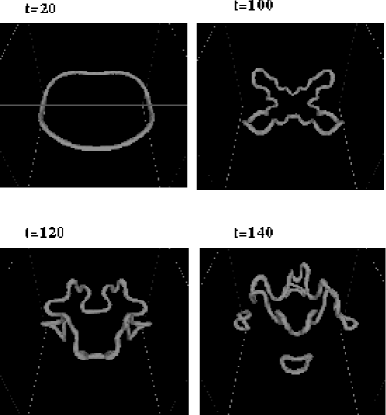
Such states are frequently observed in simulations with periodic boundary conditions (see e.g. Manneville and Chaté (1992), Popp et al (1993), Stiller et al (1995)a,b). Figure 5 shows the modulus of a typical solution found in a simulation. §§§For one expects to observe conservative dynamics for holes and shocks, similar to interacting particles for zero friction. As shown in Figure 4 one finds uniform as well as (almost) harmonic and strongly anharmonic oscillating hole velocities. (Slightly) beyond the core instability line the direction of the velocity is changed in the oscillations (see Figure 4 d). The solutions are seen to be very sensitive to –perturbations of the cubic CGLe.
The uniformly moving solutions can be well understood from the results of the last subsections. First, they are not expected to exist (and we indeed could not observe them in simulations) in the range of monotonic interaction, below curve MOH in Fig. 2, ¶¶¶The boundary between monotonic and oscillatory interaction depends on the hole velocity (see Subsec. II F). since here the asymptotic hole–shock interaction is always attractive. In the oscillatory range, and away from the core instability line uniformly moving periodically modulated solutions can then be identified as fixed points of a first-order ordinary differential equation for the hole velocity which can be derived by the matching-perturbation method (Popp et al, 1995). In addition, solutions with oscillating hole velocities were found coexisting (stably) with uniformly moving solutions (see Figures 4b, 4c). They can (in a first approximation) be identified as stable limit cycles of a two-dimensional dynamical system with the hole velocity and the hole–shock distance as active variables. These oscillations are of a different nature than those found slightly beyond the core instability line (Fig. 4d), see above.
By an analysis of the perturbed equations (44) Doelman (1995) has shown that the quintic perturbations create large families of traveling localized structures which do not exist in the cubic case.
3 Connection with experiments
Transient hole-type solutions were observed experimentally by Lega et al (1992), and Flesselles et al (1994) in the (secondary) oscillatory instability in Rayleigh-Bénard convection in an annular geometry. Here one is in a parameter range where holes are unstable in the cubic CGLe, so that small perturbations are irrelevant. Long time stable stationary holes (“1d spirals”) were observed in a quasi-1d chemical reaction system (CIMA reaction) undergoing a Hopf bifurcation by Perraud et al (1993). The experiments were performed in the vicinity of the cross-over (codimension-2 point) from the (spatially homogeneous) Hopf bifurcation to the spatially periodic, stationary Turing instability. Simulations of a reaction-diffusion system (Brusselator) with appropriately chosen parameters exhibited the hole solutions (and in addition more complicated localized solutions with the Turing pattern appearing in the core region). Strong experimental evidence for Nozaki-Bekki holes in hydrothermal nonlinear waves is given by Burguette et al (1999).
Finally we mention experiments by Leweke and Provensal (1994), where the CGLe is used to describe results of open-flow experiments on the transitions in the wake of a bluff body in an annular geometry. Here the sensitive parameter range is reached and in the observed amplitude turbulent states holes should play an important role.
C Other coherent structures
Coherent states (41) with periodic functions and (same period) have been of particular interest. In general, when the spatial average of is nonzero, the complex amplitude is quasiperiodic, i.e. can be written in the form (14) with a periodic function of . The associated wavenumber will be called the “inner wavenumber”, in contrast to the outer wavenumber , which is equal to the spatial average of . These quasiperiodic solutions bifurcate from the traveling waves (20) in the Eckhaus unstable range at the neutrally stable positions obtained from Eq. (22) with and replaced by . In fact, the long-wave Eckhaus instability is signalizes in particular by bifurcations of the solitary (or homoclinic) limit solution . In this limit the velocity is at the bifurcation equal to the group velocity , see Eq. (25).
Well away from the Benjamin-Feir-Newell instability (on the stable side) the bifurcation is subcritical (as for the GLe). However, it becomes supercritical before the Benjamin-Feir-Newell line is reached (Janiaud et al (1992)) and remains so in the unstable range. The bifurcation is captured analytically most easily in the long-wave limit by phase equations, see Subsec. II G. The supercritical nature of the bifurcation allows to understand the existence of “phase chaos” that is found when the Benjamin-Feir-Newell line is crossed (see below).
1 The GLe and NLSe
For the GLe a full local and global bifurcation analysis is possible and the quasi-periodic solutions can be expressed in terms of elliptic functions (Kramer and Zimmermann, 1985; Tuckerman and Barkley, 1990). Indeed, for Eqs. (44) lead to the second-order system
| (57) |
with an integration constant. This allows to invoke the mechanical analog of a point particle (position , time ) moving in the potential . On sees that for the potential has extrema at with corresponding to the plane-wave solutions (20) with , . The maximum corresponds to . It is stable since it correspond to a minimum of . The solution is unstable. In this way the Eckhaus instability is recovered. The bifurcations of the quasi-periodic solutions are subcritical and the solutions are all unstable. They represent the saddle points separating (stable) periodic solutions of different wavenumber, and thus characterize the barriers against wavelength-changing processes involving phase slips.
As was already mentioned in the Sec. II, all stationary solutions and their stability properties of the 1D (defocusing) NLSe coincides with those of the GLe. In addition, the NLSe has more classes of coherent structures due to the additional Galilean and scaling invariance absent in GLe. We will not touch this question since the 1D NLSe is a fully integrable system (Zakharov and Shabat, 1971) that has been studied in great detail (see, e.g. Proceedings of Conference on The Nonlinear Schrödinger Equation (1994)).
2 The CGLe
For the CGLe the local bifurcation analysis has been first carried out in the limit of small using the phase equation (35) (Janiaud et al 1992) and subsequently for arbitrary (Hager and Kramer, 1996). It shows that the Eckhaus instability becomes supercritical slightly before the Benjamin-Feir-Newell curve is reached. The bifurcation has in the long-wave limit a rather intricate structure, since the limits and do not interchange (this can already be seen in the GLe). When taking first the solitonic limit (while ) the Eckhaus instability becomes supercritical slightly later than in the other (“standard”) case, which corresponds to harmonic bifurcating solutions. These features are captured nicely by the phase equation description.
Recently Brusch et al (2000) carried out a systematic numerical bifurcation analysis based on Eqs. (44) for the case , where is periodic (nevertheless we will usually refer to these solutions as quasi-periodic solutions). It shows that the supercritically bifurcating quasi-periodic branch (shallow quasi-periodic solutions) terminates in a saddle-node bifurcation and merges there with an “upper” branch (deep quasi-periodic solutions), see Fig. 6. For the bifurcating solution has velocity (in Eqs. (44) the bifurcation is of Hopf type). It is followed by a drift-pitchfork bifurcation generating a nonzero velocity. The separation between the two bifurcations tends to zero for vanishing , so that the solitary solutions develop a drift from the beginning on (at second order in the amplitude). ∥∥∥for there is drift already after the first bifurcation, so the drift-pitchfork gets unfolded (Brusch, private communication). These features can be reproduced by the Kuramoto-Sivashinsky equation, which only exhibits the shallow homoclons. By adding higher-order (nonlinear) terms (Sakaguchi, 1990) the other branch can be generated. Brusch et al (2000) give evidence that the existence of the two branches provides a mechanism for the stabilization of phase chaos (see below).
Deep quasi-periodic solutions (in the solitary limit) were first studied by van Hecke (1998) and then by van Hecke and Howard (2001) in the context of spatio-temporal chaos in the intermittent regime (see next subsection). Following this author we have adopted the name “homoclons” for the localized objects.
The stability properties of quasi-periodic solutions were also analyzed by Brusch et al., 2000. Both branches of quasi-periodic solutions have neutral modes corresponding to translation and phase symmetries. The eigenvalue associated with the saddle-node bifurcation is positive for deep homoclons and negative for shallow ones. Apart from these three purely real eigenvalues, the spectrum consists of complex conjugated pairs.
For not too small wavenumber all the eigenvalues of the shallow branch are stable within a system of length , but when increases, the quasi-periodic solutions may become unstable with respect finite-wavelength instabilities (near the bifurcation they certainly do).
Shallow quasi-periodic solutions can be observed in simulations of the CGLe (away from the bifurcation from the plane waves), in particular for (Janiaud et al, 1992; Montagne, et al 1996, 1997; Torcini, 1996; Torcini, Fraunkron, and Grassberger, 1997).
Also more complex coherent structures, corresponding to nonperiodic arrangements of shallow homoclons were found numerically. They can be understood from the fact that the interaction between shallow homoclons can be of oscillatory nature depending on parameters. This is suggested by the fact that in the supercritical regime the spatial exponents introduced in Sec. II F are complex. Clearly chaotic solutions may be expected to exist in Eqs. (44).
D Spatio-temporal chaos
1 Phase chaos and the transition to defect chaos
When crossing the Benjamin-Feir-Newell line with initial conditions (actually any nonzero, spatially constant is equivalent) one first encounters phase chaos, which persists approximately in the lower dashed region between Benjamin-Feir-Newell and absolute instability curves in Fig. 2. In this spatio-temporally chaotic state remains saturated (typically above about ) so there is long-range phase coherence and the global phase difference (here equal to ) is conserved. In this parameter range one also has stable, periodic solutions, but they obviously have a small domain of attraction which is not reached by typical initial conditions. Beyond this range phase slips occur and a state with a nonzero (average) rate of phase slips is established (defect or amplitude chaos). Since in phase chaos only the phase is dynamically active it can be described by phase equations (in the case of zero global phase the the Kuramoto-Sivashinsky equation, otherwise Eq. (35)).
In the CGLe, phase chaos and the transition to defect chaos (see below), was first studied by Sakaguchi (1990) and subsequently systematically in a large parameter range by Shraiman et al (1992) and for selected parameters and in particular very large systems by Egolf and Greenside (1995). One of the interests driving these studies was the question if in phase chaos the rate of phase slips is really zero, so it could represent a separate phase (in the thermodynamic sense), or if the rate is only very small. The recent studies by Brusch et al (2000) on the quasi-periodic solutions with small modulation wavenumber (see subsec. III C 2) point to a mechanism that prevents phase slips in a well-defined parameter range.
In fact, phase chaos “lives” on a function space spanned by the forwardly bifurcating branches of the quasi-periodic solutions. Thus, snapshots of phase chaos can be characterized (roughly) as a disordered array of shallow homoclons (or “disordered quasi-periodic solutions”), see Fig. 7. The dynamics can be described in terms of birth and death processes of homoclonal units. When these branches are terminated by the saddle-node bifurcation, phase-slip processes are bound to occur. Brusch et al (2000) have substantiated this concept by extensive numerical tests with system sizes ranging from to and integration times up to . For a given (not too small) phase slips occurred only past the saddle-node for the quasi-periodic solutions with inner wavenumber . Tracking of (rare) phase-slip events corroborated the picture. Thus, the authors conjectured that the saddle-node line for provides a strict lower boundary for the transition from phase to defect chaos.
One expects existence of a continuous family of two types of phase chaos with different background wavenumbers . For the state should arise when crossing the Eckhaus boundary for the plane wave with wavenumber , before the Benjamin-Feir-Newell limit. Such states were studied by Montagne et al (1996,1997) and Torcini (1996) and Torcini et al (1997). It was found that the parameter range exhibiting phase chaos decreases with increasing . Thus, at fixed parameters , one has a band of phase chaotic states which is bounded from above by some . Approaching the limit of phase chaos, decreases smoothly to zero, i.e. the phase chaotic state with is the last to loose stability, similar to the situation for the plane waves. As mentioned before, for not too small , one finds coexistence with quasi-periodic solutions and spatially disordered coherent states.
2 Defect chaos
The transition (or crossover) between phase and defect chaos is reversible only for larger than about (near the lower edge of Fig. 2) [Shraiman et al, (1992)]. There, when approaching the transition from the side of defect chaos, the phase slip rate goes smoothly to zero. On the other hand, for , there is a region where phase and defect chaos coexist (“bichaos”, lower dashed region to the right of line DC), and in fact defect chaos even persists into the Benjamin-Feir-Newell stable range (the limit towards small is approximated by the dashed line DC in Fig. 2) (Shraiman et al, 1992; Chaté, 1993; Chaté and Mannneville, 1994). There the defect chaos takes on the form of spatio-temporal intermittency.
A qualitative understanding of the parameter region where one has bistable defect chaos can be obtained as follows: In this region, starting from the (”saturated”) state with and forcing a large excursion of leading to a phase slip, makes it easier for other phase slips to follow. This memory effect is suppressed with increasing as can be seen from the increase of the velocity with of fronts that tend to restore a saturated state (see Sec. III A).
From above (towards small values of ) the chaotic state joins up with the region of stable Nozaki-Bekki holes. The characteristics of these holes is influenced by small perturbations of the CGLe, and this in turn affects the precise boundary of of spatio-temporal chaos, see Subsec. III D 4.
3 The intermittency regime
This regime where defect chaos coexists with stable plane waves has been studied numerically in detail by Chaté (1993, 1994) and he has pointed out the relation with spatio-temporal intermittency. There, typical states consist of patches of plane waves, separated by various localized structures characterized by a depression of . The localized structures can apparently be divided into two groups depending on the wavenumbers and of the asymptotic waves they connect. On one hand one has slowly moving structures which can be related to Nozaki-Bekki holes, which in this regime are either core stable or have long lifetime. They become typical as the range of stable Nozaki-Bekki holes is approached (Chaté, 1993, 1994).
However, in a larger range the dominant local structures have velocities and asymptotic wavenumbers that are incompatible with the Nozaki-Bekki holes and which, according to van Hecke (1998), must be associated with the deep homoclons. Space-time plots of the amplitude , the phase (), and the local wavenumber in such a regime are shown in Fig. 8 (the plot is a zoom in of a larger simulation as shown in Fig. 9b). The wavenumbers of the laminar patches are quite close to zero, while the cores of the local structures are characterized by a sharp phase-gradient (peak in ) and dip of ). The holes propagate with a speed of and either their phase gradient spreads out and the hole decays, or the phase-gradient steepens and the hole evolves to a phase slip. The phase slip then sends out one (or maybe two) new localized objects which repeat the process. Van Hecke (1998) provides evidence that the dynamics evolves for much of the time around the one-dimensional unstable manifold of homoclons with background wavenumber near zero. They provide the saddle-points that separate dynamical processes which lead to phase slips from those that lead back to the (laminar) plane-wave state. When the parameters and are quenched in the direction of the transition to plain waves, these zigzag motions of the holes becomes very rapid (Fig. 9a).
Additional consideration of homoclons and their role in spatio-temporal chaos is presented by van Hecke and Howard, 2001. The simulations of the CGLe show that when an unstable hole invades a plane wave state, defects are nucleated in a regular, periodic fashion, and new holes can then be born from these defects. Relations between the holes and defects obtained from a detailed numerical study of these periodic states are incorporated into a simple analytic description of isolated “edge” holes, which are seen in Fig. 9.
Recently Ipsen and van Hecke (2001) found in long-time simulations that in restricted parameter range composite zigzag patterns formed by periodically oscillating homoclinic holes represent the attractor.
4 The boundary of defect chaos towards Nozaki-Bekki holes
As the boundary of stability of Nozaki-Bekki holes is approached (curve AH in Fig. 2) one can increasingly observe Nozaki-Bekki hole-like structures that emit waves and thereby organize (“laminarize”) their neighborhood. In this regime the state becomes sensitive to small perturbations of the cubic CGLe, as discussed in Sec. III B.
It is found that stable hole solutions suppress spatio-temporal chaos and as a consequence, for a decelerating ( if ) perturbation, the (upper) boundary of spatio-temporal chaos is simply given by the stability boundary AS in Fig. 2 of the Nozaki-Bekki hole solutions, whereas for an accelerating perturbation spatio-temporal chaos is also observed further up (Popp et al 1993; Stiller et al 1995b). For random initial conditions lead to an irregular grid of the standing holes, separated by shocks from each other, see Fig. 10b. Such grids are the 1D analog of the “vortex glass” state found in 2D (see Subsec. IV G), see also Chaté, 1993.
Clearly, for accelerating such a grid is unstable. In this case Nozaki-Bekki holes are created from random initial conditions, too. In their neighborhood they suppress small-scale variations of typical for amplitude chaos in the major part of the chaotic regime. However, since they are accelerated they only have finite life time, see Figure 10a. For parameters below about curve EH in Fig. 2 (the coincidence with the Eckhaus limit presumably fortuitous) the destruction of the holes leads to creation of new holes and shocks, yielding a chaotic scenario of subsequent acceleration, destruction and creation processes.
IV Dynamics in 2D
A Introduction
The 2D CGLe has a variety of coherent structures. In addition to the quasi-1D solutions derived from the coherent structures in 1D discussed above the CGLe possesses localized sources in 2D known as spiral waves. An isolated spiral solution is of the form
| (58) |
where are polar coordinates. The (nonzero) integer is the topological charge, and is the (rigid) rotation frequency of the spiral, is the amplitude and is the phase of the spiral, for is the asymptotic wavenumber selected by the spiral (Hagan 1982), and is the spiral frequency ******Spirals with zero topological charge (targets) are unstable in the CGLe. However, inhomogeneities can stabilize the target. Hagan (1981) have found stable targets in the inhomogeneous CGLe in the limit of small . Stationary and breathing targets in the wide parameter range of the CGLe were studied by Hendrey et al (2000). Since spirals emit asymptotically plane waves (group velocity ), they are source solution. In addition to spirals there exist sinks which absorb waves. The form of sinks is determined by the configuration of surrounding sources. Sinks with topological charge appear as edge vortices (see below). Spiral solutions with are unstable (Hagan, 1982). Single-charged spiral solutions are dynamically stable in certain regions of parameter space. The grey-coded image of a spiral and an edge vortex is shown in Fig. 11. For , and also for , the asymptotic wavenumber of the spiral vanishes and the solution goes over into the well-known vortex solution of the GLe and NLSe, known in the context of superfluidity (Pitaevskii,1961, Gross 1963, Donnelly, 1991) and somewhat similar to that found in superconductivity in the London limit (Abrikosov, 1988, Blatter et al 1994). In periodic patterns spirals and vortices become dislocations.
The asymptotic interaction is very different for the case , where it it is long range decaying like with some corrections, whereas for it is short range decaying exponentially (see below). Interaction manifests itself in a motion of each spiral. The resulting velocity can have a radial (along the line connecting the spiral cores) and a tangential component.
Spirals may form regular lattices and/or disordered quasi-stationary structures called vortex glass or frozen state. When individual spirals become unstable (spiral break-up), the typical spatio-temporal behavior is chaotic.
B Spiral stability
1 Outer stability
For spirals to be stable the wavenumber of the asymptotic plane wave has to be in the absolutely stable range (see Sec. II E). In order to find this stability limit we have to evaluate the condition (32) for the wavenumber emitted by the spiral, see Fig. 12. Existence of an absolutely stable spiral solution guarantees that small perturbations within the spiral will decay, but does not assure that it will evolve from generic initial conditions. For further discussion see Sec.IV H 2.
2 Core Instability
The spiral core may become unstable in a parameter range where diffusive effects are weak compared to dispersion (large limit). Then it is convenient to rewrite CGLe in the form
| (59) |
where and length has been rescaled by . This situation is typical in nonlinear optics (transversely extended lasers or passive nonlinear media). In this case a systematic derivation of the CGLe from the Maxwell-Bloch equations in the ”good cavity limit” for positive detuning between the cavity resonance and the atomic line leads to very small values of (Coullet et al 1989a; Oppo et al 1991; Newell and Moloney, 1992; Newell, 1994). Representative values are (Coullet et. al, 1989a).
For one has the Galilean invariance mentioned in Sec.II C, (see Saarloos and Hohenberg, 1992, for the 1D case) and then in addition to the stationary spiral there exists a family of spirals moving with arbitrary constant velocity
| (60) |
where , , and the functions are those of Eq. (58) (this invariance holds for any stationary solution). For the diffusion term destroys the family and in fact leads to ac- or deceleration of the spiral proportional to . The natural assumption is that one has deceleration so that the stationary spiral is stable (Coullet et. al, 1989a). In fact this is not the case. Stable spirals exist only above some critical value . Below the stationary spirals are unstable with respect to spontaneous acceleration (Aranson et al, 1994).
For small values of one may expect the solution (60) to be slightly perturbed and have a slowly varying velocity which obeys an equation of motion of the form . Because of isotropy the elements of the tensor must satisfy and , so the relation can also be written as
| (61) |
where and . Since in general the friction constant is complex the spiral core moves on a (logarithmic) spiral trajectory.
The acceleration instability of the spiral core has a well-known counterpart in excitable media, where the spiral ”tip” can perform a quasiperiodic motion leading to meandering (see, e.g. Barkley, 1994). The main difference between the two cases can be understood by considering the nonlinear extension of Eq. (61) with . In excitable media one has , which provides the saturation of the instability. On the other hand, in CGLe the sign of is opposite and destabilizes the core according to simulations. Thus one has an alternative scenario of the meandering instability. The scenario appears to be generic and is not destroyed by small perturbations of the CGLe.
Now going to larger one finds that increases with and finally changes sign at a value . The result obtained from extensive numerical simulations is shown in Fig. 13.
The acceleration instability can also be interpreted as the destabilization of a localized core mode similar to the situation of the standing hole solution in the 1d CGLe (Popp et al, 1993, Sasa and Iwamoto, 1993; Chaté and Manneville, 1992, see Sec. III).
The case of negative diffusion ( ) is important especially for lasers with negative detuning (Oppo, 1991; Staliunas, 1993; Lega et al, 1994). Then higher-order corrections to the diffusion (fourth derivative) have to be included to stabilize the short-wave instability. The resulting complex Swift-Hohenberg equation is
| (62) |
This equation exhibits in some range of parameters a similar core instability. In a certain parameter range one has stable meandering of the spiral (Aranson and Tsimring, 1995; Aranson, Hochheiser, and Moloney, 1997)
C Dynamics of vortices in the GLe, NLSe, and for
1 Dynamics of vortices in GLe
In the GLe the spirals become vortices, i.e in Eq. (58) one has and . is a monotonic function and for , for .
A more general isolated moving vortex solution with wavevector away from band center is described by :
| (63) |
where fulfills the boundary conditions for with the appropriate phase jump of . ††††††It is important to mention that such a problem is not well defined for spiral waves (). Since the spiral waves are active sources they can in general not coexist with the plane waves. Depending on the relation between the two frequencies either the spiral would invade the entire plane or the plane wave would push the spiral away. For details see Sec. IV F
For large systems such that , where is the system size or the distance to another defect, the drift velocity is perpendicular to the background wavenumber , such that the free energy decreases. The speed is given by the expression
| (64) |
with the constant (see Bodenschatz et al, 1988b, 1991, Kramer et al, 1990). Here is the rotation matrix
The term in the brackets on the rhs has been fitted to numerical results (see Bodenschatz et al. 1991). The formula can be used throughout the stable range and is consistent with experiments of Rasenat et al (1990) in electroconvection in nematics. In small systems , the velocity is given by with .
The above relations were rederived by Pismen and Rodriguez (1991), Rodriguez and Pismen (1991), Ryskin and Kremenetsky (1991), and in part by Neu (1990a) using matching asymptotics techniques.
The result shows that for an isolated defect the limits of the system size going to infinity and wavenumber mismatch (or defect velocity) going to zero are not interchangeable. This is analogous to the 2D-analog of Stokes’ law (drag of an infinite cylinder through an incompressible fluid), where one also has a logarithmic divergence of the mobility at vanishing velocities. The similarity was pointed out by Ryskin and Kremenetsky (1991). It is also useful to note that the force exerted on dislocations in a phase gradient expressed by a wave vector is the analog of the well-known Peach-Koehler force on dislocations in crystals under stress.
In the following we consider linearly stable periodic states, where . All periodic states, except (band center), are metastable. Evolution to the band center can occur by the motion of vortices, once they have been nucleated by finite fluctuations or disturbances (see Bodenschatz et al., 1988b, and Hernandez-Garcia et al, 1993, for a discussion of the problem of homogeneous nucleation of vortices).
The asymptotic interaction between two vortices can be described approximately by Eq. (64) with the r.h.s. replaced by the gradient of the resulting phase of other vortex at the center of the vortex. Since the gradient is perpendicular to the line connecting the vortex cores, the resulting force is directed along this line. As a result, oppositely-charged vortex attract each other and eventually annihilate, whereas like-charged repel each other.
The analysis of an isolated moving vortex shows that the deformation of the roll pattern decays in front exponentially over a distance , while behind the dislocation the decay is proportional to . Thus, if the background wavenumber is nonzero and two vortices with opposite topological charge are approaching each other, the velocity will be constant for . Subsequently the motion will accelerate and eventually the attraction will dominate over the Peach-Koehler force and lead to annihilation. ‡‡‡‡‡‡In this discussion we have tacitly considered the situation where the Peach-Koehler force and the force due to interaction are parallel to each other. If this is not the case the vortices will move on curved trajectories. In experiments by Brawn and Steinberg (1991), the annihilation process was studied in detail near the band center () where accurate determination of is not possible. The quantitative comparison with theory is shown in Fig. 14 where the distance between two vortices of opposite polarity approaching each other along a straight line versus time is shown for different in scaled units, (Bodenschatz et al, 1991). At time the vortices annihilate. The solid line gives the numerical results, and the squares, circles and diamonds are the experimental data.
The case , where the Peach-Koehler force vanishes so that for , deserves special attention. The analysis of Bodenschatz et al (1988)b, leads to , where for . Clearly for this to hold needs to be exponentially large. Otherwise one is caught in the intermediate region where no accurate relation for was found. For that reason the so-called self-consistent approximation was proposed by Pismen and Rodriguez (1990), Rodriguez and Pismen (1991), Pismen (1999):
| (65) |
where the sign corresponds to a like-charged pair, the sign to an oppositely-charged one, and and are modified Bessel functions. The formula is not very accurate, as shown by comparison with full simulations (Weber, 1991, 1992a).
Allowing for a very small wavevector displacement , one finds . One can then get to the limit and then, for sufficiently large systems, .
For small distances, shortly before annihilation of an oppositely charged pair, the gradient terms in the GLe become dominant and one may argue that the dynamics is governed by self-similar solutions of the diffusion equation so that , which appears consistent with the numeric results.
2 Dynamics of vortices in the NLSe
Although the stationary vortex solution of the NLSe coincides with that of GLe, the dynamic behavior of NLSe is very different from that of the GLe and is similar in the limit of small velocities, large separation, and properly quantized circulation to the motion of point vortices in an ideal incompressible fluid (Lamb, 1932). The problem of the vortex motion in the context of the NLSe was first considered by Fetter (1966), and then many researchers rederived this result more accuracy (see, e.g. Creswick and Morrison, 1980; Neu, 1990b; Lund, 1991, Pismen and Rubinstein, 1991a, Rubinstein and Pismen, 1994).
Introducing the amplitude-phase representation and the “superfluid density” as well as the superfluid velocity one obtains from Eq. (6) an Euler equation
| (66) |
and the continuity equation for the “density” of superfluid
| (67) |
Here is the effective “pressure”, whereas the first term is called “quantum pressure”. The quantum pressure is irrelevant for large-scale perturbations of the density, i.e. . In the Euler equation incompressibility approximation is reliable for the velocities much smaller than the sound velocity . One expects the analogy with classical incompressible vortex tubes in a liquid to hold for the well-separated vortices moving with the velocity . Thus, according to classical hydrodynamics ( Lamb, 1932), one obtains that the oppositely charged vortex pair drifts with the velocity normal to the line connecting the cores of the vortices, and like-charged pair rotates around the center of the symmetry, where is the distance between vortex center. This result up to higher order corrections holds for well separated vortices () in the NLSe, as it was rederived later on by Neu (1990)b, Pismen and Rubinstein (1991), and by Rubinstein and Pismen (1994), using matching asymptotic technique. Numerical investigation of vortex dynamics in the NLSe was carried out also by Nore et al (1993), Frisch et al (1992), Abraham et al (1995), Josserand and Pomeau (1995).
For well-separated vortices located at the points one has the more general formula
| (68) |
According to Eq. (68), obtained from the corresponding incompressible Euler equation, the vortex velocities diverge as the intervortex distances vanish. However, the above expression becomes incorrect when the inter-vortex distance becomes of the order of the coherence length (one in our scaling). For small separations the interaction of two like-charged vortices can be considered as a small perturbation of a double-charged vortex. Aranson and Steinberg (1995) have shown that for the velocity of vortices vanishes, and the frequency of rotation for like-charged vortex pair approaches a constant as (the “classical formula” (68) results in infinite frequency). Similarly, for an oppositely charged pair the velocity remains finite for .
An important problem in the context of NLSe is the nucleation (or generation) of vortices from zero-vorticity flow. Frisch, Pomeau, and Rica (1992) considered the stability of flow passing an obstacle and found nucleation of vortex pairs above some critical velocity. Yet another mechanism of vortex generation is related to the instability of quasi-1D dark solitons, predicted by Kuznetsov and Turitsyn (1988). Josserand and Pomeau (1995) studied the instability of dark solitons numerically and found that the nonlinear stage of this instability results in creation of vortex pairs.
3 Dynamics of vortices for
The general case , including the NLSe limit, can be related to the GLe limit by generalizing the ansatz (63) to
| (69) |
Eq. (1) can be written as
| (70) |
After neglecting the higher-order term , one observes that Eq. (70) coincides with the corresponding equation for if one replaces by . ******The calculations can be generalized to arbitrary .
As a result we may extend the expression (64) for arbitrary leading to
| (71) |
One obtains oblique motion with respect to with the angle depending on and . In the NLSe limit the motion becomes parallel to . Concerning the interaction between vortices one obtains oblique repulsion or attraction: for two vortices never move along the line connecting their centers but instead spiral with respect each other (Pismen, 1999).
D Dynamics of spiral waves for
1 General
As we mentioned above, in the generic case of the asymptotic interaction of topological defects (spirals) is very different from the corresponding dynamics of vortices in GLe and in NLSe. The problem of spiral wave interaction was considered by Biktashev (1989), Rica and Tirapegui (1990),(1991)a,b,(1992), Elphick and Meron (1991), Aranson et al (1991),(1993)a, Pismen and Nepomnyashchii (1991)a,b. The approach of Rica and Tirapegui (1990),(1991)a and Elphick and Meron (1991), explored a type of global phase approximation which in essence gave long-range interaction between the spirals, in analogy to the cases treated above. The results were in obvious disagreement with numerical simulations done by Aranson et al (1991), revealing exponentially weak interaction between the spirals.
A more adequate solution of the problem was obtained later by Aranson et al (1991), and Pismen and Nepomnyashchii (1991)a,b, on the basis of the phase diffusion equation (see also Biktashev, 1989). The results demonstrated an exponentially weak asymptotic interaction, although they failed to describe the numerically observed bound states of spiral waves. The abovementioned approach is adequate for the case . Biktashev (1989) considered a the very restrictive problem of spiral motion in an almost-circular domain. Due to some unphysical boundary conditions the results of Pismen and Nepomnyashchii (1991),(1992), were at conflict with numerical simulations (Aranson et al 1993a).
In later papers Rica and Tirapegui (1991)b,(1992) attempted to improve their interaction approach by combining it with that of Aranson et al (1991). However, in our view, the results remain unsatisfactory because of an uncontrolled perturbation technique.
A consistent theory with quantitative predictions of asymptotic spiral wave interaction including bound-state formation was presented by Aranson et al (1993)a,b using the matching perturbation method. The idea of the method is straightforward: in the full solutions for a spiral pair (or a spiral and a wall, or more complicated aggregates of spirals) the spirals move with certain velocities, and thus solutions exist only with the “correct” velocities. Such solutions may be constructed approximately by starting with isolated spirals, each one restricted to the region in space filled by its emitted waves and moving with (small) velocities to be determined. For a symmetric spiral pair one simply has two half planes. In a first step the corrections are assumed to be determined to sufficient accuracy by the linearized (perturbational) problem with boundary conditions that take into account the neighboring spiral (or wall etc.). The velocity comes in as an inhomogeneity. The occurrence of bound states can already be seen from the behavior of stationary perturbations of the asymptotic plane waves emitted by the spirals, as given by Eq. (33). Bounds states occur in the oscillatory regime, outside the curves (one must choose the curves inside the Benjamin-Feir-Newell-stable region). The oscillatory range is plotted in Fig. 12 (curve ). Also included in Fig. 12 is the convective Eckhaus-stability boundary (curve , see Sec. II D) and the boundary of absolute stability (curve , see Sec. II E) for the waves emitted by the spirals.
The inhomogeneities involve the velocity linearly and as a consequence the solution for arbitrary (but not too small) distance can be expressed in terms of one inhomogeneous and a homogeneous solution. Once these are determined numerically and used to match the boundary conditions the velocity versus distance relation comes out. For (for simplicity) the resulting velocities of the spiral at distance from a plane boundary (or, equivalently, a pair of oppositely-charged spirals at the points ) are of the form
| (72) | |||||
| (73) |
where is the spiral wavenumber, is the component of the velocity along the line connecting spiral cores (radial velocity) and is the velocity perpendicular to this line (tangential velocity). The constants and are obtained numerically and the parameter is derived from the linearized problem (Aranson et al, 1993a). The bound states correspond to the case of . The bound state will drift with the velocity . The equilibrium distance between the spirals is found from the equation
| (74) |
Since only and are complex this gives
| (75) |
where and . Even values of correspond to stable bound states, odd to unstable ones. Usually the lowest bound state with is relevant. Approaching the boundary of the oscillatory range the equilibrium distance diverges.
Generalization to arbitrary can be done along the lines of the similarity transformation (19). The result is at leading order unchanged. *†*†*†Note that the additional term arising in the corresponding equations of motion for each spiral can be absorbed in the nonsingular part of the linear problem (Aranson and Pismen, 2000).
Note that the symmetries (like-charged) and (oppositely-charged) have nearly the same effect on the boundary conditions at for large spiral separation. Thus for large separation the interaction of like-charged spirals is similar to the interaction of oppositely-charged ones. The only difference is that for the like-charged case both components of the velocities of the spirals have opposite sign whereas for the oppositely-charged case the tangential components have the same sign. This causes the rotation of the spirals around the common center of the symmetry in the like-charged case.
Like-charged spirals may form more complicated bound states or aggregates. In contrast to the two-spiral bound states, which are simply rotating with constant velocity, each spiral in the aggregate performs a more complicated motion (possibly nonperiodic) on the background of a steady-state rotation, perhaps similar to the ”dance” of spiral aggregates observed in a variant of the Belousov-Zhabotinsky reaction (Steinbock and Müller, 1993). Certain problems of interaction between spiral waves and hole solutions were considered by Bazhenov and Rabinovich (1993,1994). Interaction of spiral with external periodic perturbation and response functions of the spiral core were studied by Biktasheva et al (1998,1999,2000).
2 Comparison with results of numerical simulations
Bound states of spirals are shown in Fig. 15. In Fig. 16a the dependence of the velocities on the spiral separation is plotted for and compared with results from full numerical simulations. There is reasonable agreement, particularly for the radial velocity . The first two zeros of at and correspond to in Eq. (75). Here the velocities are already extremely small. From the simulations no other bound state could be resolved. The equilibrium distance obtained from the theory for the stable bound state ( in Eq. (75)) is in a very good agreement with the results of the simulations of the full CGLe (see Fig. 16a). There is a discrepancy between the values of the tangential velocity by a factor of about (see Fig. 16b) although the functional dependencies on are very similar. This discrepancy results from the fact that the shock is not described well in linear treatment.
More accurate estimates can be obtained by treating the shock fully nonlinearly. Far away from the core the motion of the spiral can be neglected and one may consider the stationary shock produced by the waves emitted by the spirals. Thus one has to solve the stationary CGLe with boundary conditions for , and at . This is a rather complicated 2D problem. Numerically one could extract more accurate values of the constants , characterizing reflection at the shock, see Fig. 16b.
3 Interaction in the monotonic range.
In the case there exist two real positive roots of Eq. (33). Using the analogous numerical procedure one can also determine the constants , but for small it is technically very difficult in this form. The results can be simplified considerably for the case and . Then one can neglect the coefficients because for one has and . One obtains , which exhibits explicitly the exponential decay of the interaction and reproduces the earlier analysis using a phase diffusion equation (Aranson et al, 1991; Pismen and Nepomnyashchii, 1991,1992; Biktashev, 1989).
Numerical simulations for oppositely charged spirals for and indicate asymptotic repulsion (Aranson et al, 1993a). This result can be inferred already from the work of Biktashev (1989), who used a phase-diffusion equation and asymptotic matching to treat the interaction of spirals with a boundary. It appears to be at conflict with the works of Pismen and Nepomnyashchii (1991)a,b where in the limit matching with the internal solution was done analytically and asymptotic attraction was found. The repulsive range is expected to move to larger roughly as for smaller . In this way the crossover to the long-range attraction within the GLe is recovered. Interaction becomes attractive at smaller distance leading to final annihilation of the spiral pair.
Like-charged spirals for have repulsion at large distance (as in the oppositely-charged case) and also at small distance. So it is quite clear that the interaction is repulsive everywhere.
E Interaction of spirals with a inhomogeneity
Spirals may interact with inhomogeneities of the medium. This problem is particularly interesting in the context of Bose-Einstein condensation as described by the NLSe in a parabolic potential (for a review see Dalfovo et al, 1999). Weak inhomogeneities are sometimes included into the CGLe in the form
| (76) |
with an appropriate function . An interesting problem is the drift of a spiral in the gradient created by a localized, radially symmetric inhomogeneity (see Staliunas, 1992, Gil et al, 1992). The spiral may be trapped (pinned) by the inhomogeneity or perform a stationary rotation at some distance from the inhomogeneity as observed in optical systems (Arecchi, 1990, 1991; Brambilla et al, 1991).
Using the method described above one arrives at the following expression for the spiral velocity due to interaction with weak axisymmetric inhomogeneity (Aranson et al, 1993c)
| (77) |
where is the distance from the inhomogeneity to the spiral core, is the spiral core velocity and the function is obtained by a convolution of the inhomogeneity profile with the corresponding solution of linearized CGLe. Equation (77) is the analog to the motion of a ”massless particle” in a radially-symmetric field. Numerical simulations with CGLe shows that Eq. (77) describes the motion of the spiral fairly well for not too large values of , see Fig. 17a.
For large the complex trajectories of the spiral core are not captures by Eq. (77), see Figure 17b. In order to describe the numerical simulations one has to include the effective “mass” term into the equation of motion:
| (78) |
where is the friction tensor (or mobility tensor), and , see Sec. IV B 2. Although these features were obtained in the stable range (), the external forces created by the inhomogeneity can excite the weakly damped core mode. This can explain the complex motion of the spiral core observed in the presence of obstacles (Sepulchre and Babloyantz, 1993).
Spiral motion in a slowly varying (on the scale of the coherence length) inhomogeneity was considered by Hedrey et al, (1999). In this situation additional simplifications are possible. A related problem is the motion of the spiral in the presence of small thermal noise. As was shown by Aranson et al (1998), the spiral core has finite mobility and performs Brownian motion.
F Symmetry breaking
Symmetric bound states of spirals are not necessary stable. There is numerical evidence that symmetric bound states, after a sufficiently long evolution, spontaneously break the symmetry such that one spiral begins to dominate, pushing away other spirals (Lega, 1990; Weber et al, 1991a,b; Aranson et al, 1993b). Symmetry-broken states are often produced directly from random initial conditions (Aranson et al, 1993b). To understand the symmetry-breaking instability one must consider the perturbation of the relative phase, or the frequency of the waves emitted by each spiral, caused by the interaction with the other spiral. Indeed, from the analysis of CGLe it is known, that the shock (or sink) where two waves with different frequencies collide moves in the direction of smaller frequency, due to conservation of phase. This means that after sufficiently long time only the larger frequency (or equivalently the larger wavenumber , because of the dispersion relation ) dominates in a bounded system. The velocity of the motion is given by where is the group velocity of a plane-wave state. If due to the interaction the frequencies of the spirals become different, one can expect a drastic breaking of the symmetry of the system. This effect appears to be very important for the generic long-time evolution of large systems containing spirals (vortex glass).
The symmetry breaking instability of spiral pairs can be understood from the dynamics of the relative phase of the spirals . Aranson et al (1993b) derived an equation governing the phase difference between two spirals separated by the distance
| (79) |
where are the constants obtained from the linearized CGLe. The last term represents the lowest-order term of an expansion in . The constant determined numerically from Eq. (79) turns out to be positive for the (first) symmetric bound state (see Fig. 18), so that the state is unstable with respect to . According to Aranson et al (1993b), bound states are unstable with respect to symmetry breaking in the whole oscillatory range. Due to the fact that is very small, the symmetric bound state is rather long lived. As a result of the symmetry breaking only one ”free” spiral will remain, whereas the other spiral is pushed away to the boundary. Depending on the boundary conditions the second spiral will finally either annihilate at the boundary (non-flux boundary conditions, i.e. zero normal derivative on the boundary), or, with periodic boundary conditions the defect will persist for topological reasons, but reduced to a sink and enslaved in the corner of the shock structure of the free spiral (edge vortex) (see Fig. 19). This leads to an asymmetric lattice of topological defects, which appears to be stable in the oscillatory case.
The absence of symmetry breaking in the limit and can be extracted already from the paper of Hagan (1982). From this work one finds that decreasing the radius increases the spiral wavenumber, which ultimately means stability of the shocks. The stability of symmetric states together with the repulsion of the spirals indicates the possibility for the existence of symmetric (“antiferromagnetic”) lattices of spirals (or “Wigner crystal”), i.e. lattices made up of developed spirals with alternating topological charge. Such lattices were obtained in numerical simulations in this range by Aranson et al (1993b). They appear to exist in the whole non-oscillatory range *‡*‡*‡Aranson et al (1993b) have found stable square lattices in rather small system and for relatively small number of spiral (). There is no guarantee that similar lattices are stable in arbitrary large systems.
Since for large separation the properties of like-charged spirals are analogous to those of oppositely-charged spirals, one expects the same mechanism of symmetry breaking. Indeed for above the critical value such a breaking was observed in numerical simulations.
Certain aspects of the spiral pair dynamics were studied numerically by Komineas et al (2001). It was shown that for (symmetry breaking range) the spirals interchange partners and form new pairs. For (monotonic range) symmetric spiral states were found.
G Vortex glass
A fascinating problem concerns the effect of the symmetry breaking on the long-time behavior of large systems that evolve from random initial conditions in the parameter range where one has the oscillatory interaction and spirals. Numerical simulations, carried out by Huber et al (1992), Chaté and Manneville (1996), have shown a remarkable phenomenon: from an initially strongly turbulent state eventually spirals with a developed far field evolve. The spirals grow until the entire space is filled (see Figure 20), each spiral occupying a certain domain. The domains have various sizes and typically have a four or five-sided near polygon structure. Locally each domain boundary, represented by a shock, is nearly hyperbolic. The shocks often contain “enslaved”, or edge vortices. This state appears to persist indefinitely, although sometimes domain boundaries break and edge vortices annihilate. The state was called “vortex glass” by Huber et al (1992). Some aspects of relaxation to the vortex glass were considered by Braun and Feudel (1996).
The existence of the “vortex glass” is connected with the nonmonotonic dependence of the spiral frequency on the domain size. As one sees from Figure 21 the spiral frequency oscillates as the radius of the domain increases and approaches the asymptotic value for . (The computations were done for a radially symmetric domain, but we expect the result to be qualitatively correct for domains with arbitrary convex shape.) As a result, one has sets of domain radii corresponding to the same frequency. Neighboring domains can only coexist without (further) “symmetry breaking” if they correspond to the same spiral frequency. Ultimately one can conceive of a network of fully synchronized domains of various shapes and sizes. These are likely the ingredients necessary to explains the variability of the domain sizes observed in the quasi-stationary vortex glass. The vortex glass is presumably the global attractor also in the full convectively stable oscillatory range.
Bohr et al (1996), (1997) considered the shapes of spiral domains in the vortex glass. They found that they differ from Voronoi Polygons and obtained the form of the domain boundaries from the condition of phase continuity across the shocks. In particular, far away from the center of an unperturbed spiral, the phase is given by , where are the polar coordinates measured from the center of the spiral and is the phase constant of the spiral. If one assumes that the distance between two neighboring spirals is much larger than the wavelength , one obtains simply a hyperbola describing the shock shape: . This simple formula reproduces the structure of the spiral domains with high accuracy (see Figure 22).
H Phase and defect turbulence in two dimensions
On a rough scale, two types of turbulent behaviors can be identified in 2D: phase and defect turbulence. Defect turbulence is characterized by persistent creation and annihilation of point defects. By contrast, in phase turbulence no defects occur. In the system with periodic boundary conditions the total phase gradient across the system (the “winding number”) is conserved. The simulations of Manneville and Chaté (1996) provide some evidence that phase turbulence breaks down in the infinite size, infinite time limit. However, it could be that the transition is characterized by a “sharp” bifurcation scenario similar to the situation in 1D (see III D 1).
1 Transition lines
The most detailed survey of various regimes occurring in 2D is given by Chaté and Manneville (1996) and Manneville and Chaté (1996). According to Chaté and Manneville (1996), the transition from vortex glass to defect turbulence starting from random initial conditions occurs at the numerically determined line “T”, see Fig. 12. The transition occurs somewhat prior to the absolute instability limit given from the linear stability analysis of plane waves emitted by spirals. However, starting from carefully prepared initial conditions in the form of large spirals one can approach the absolute instability limit.
Before the line “T”one finds transient defect turbulence which finally exhibits spontaneous nucleation of spirals from the “turbulent sea”. At the line “T” the nucleation time presumably diverges. Before the line “T” the entire space will finally be filled by “large spirals” separated by shocks, forming a vortex glass state.
As in 1D, persistent phase turbulence exists also in 2D between the Benjamin-Feir-Newell line and the line “L” (Chaté and Manneville, 1996; Manneville and Chaté, 1996). The range is somewhat smaller than in 1D. Beyond the line “L” defects are created spontaneously leading to defect chaos. Actually, in 2D, phase turbulence is always metastable with respect to defect turbulence or vortex glass.
2 Spiral break-up
Spiral break-up was observed in experiments on chemical oscillatory media by Ouyang and Flesselles (1996), Zhou and Ouyang (2000), in simulations of CGLe by Chaté and Manneville (1996) and model reaction-diffusion systems by Bär and Or-Guil (1999). The instability likely originates from the outer region of the spiral and thus is expected to occur beyond the line “T”. Quenching a large spiral to this domain will usually trigger a breakup scenario. On the other hand, a careful adiabatic procedure allows, in principle, to avoid breakup and to preserve one large spiral up to the (linear) absolute instability threshold. (In the presence of noise, the convective instability actually imposes a maximal noise-dependent radius .) Not too far from the absolute instability limit one is left with a smaller spiral surrounded by strong chaos (Fig. 20, left) whose well-defined radius does not depend on system size and/or distance to the boundaries but vanishes as one approaches the absolute instability threshold.
In the experiments and in some model systems, a spiral need not be introduced initially, as the chaotic phase is only metastable to the spontaneous nucleation of spirals whose radius grows up to . Thus, the asymptotic configuration on a long time scale is actually a quasi-frozen cellular state (Fig. 20, right).
The above concept of spiral break-up in large systems is in contrast to arguments by Tobias and Knobloch (1998), who stated that the spiral wave breakup occurs in the regime of absolute Eckhaus instability via “a globally unstable wall-mode confined to the outer boundary” whose front structure is at the origin of the stable “laminar” spirals immersed in a turbulent sea. Whereas a stationary front can indeed be associated with the absolute stability limit (see Sec.II E) it can only give an upper limit to the existence of the convectively unstable state.
In the break-up scenario studied by Zhou and Ouyang (2000) spirals emitting modulated waves in the presence of stable meandering of the core were observed. This behavior can be understood in terms of spatial amplification of periodic perturbations due to core meandering in the regime of convective instability of the background waves (Brusch et al., 2001). Although the saturated meandering does not occur in the framework of the CGLe, a properly perturbed CGLe may exhibit both, saturated meandering and convective instability, see Aranson, Hochheiser and Moloney (1997).
3 Defects statistics
Defect turbulence is the most chaotic state in 2D. It is characterized by exponential decay of correlations, with short correlation lengths and times. The density of defects varies with and . However, it can be argued that, at least in the most studied region with of order one, the defects do not play the role of “particle-like” excitations in this case. Indeed, the defects in the defect turbulence are very different from spiral waves since they don’t emit waves. They behave as passive objects and are merely advected by the surrounding chaotic fluctuations. According to Chaté and Manneville (1996) “amplitude turbulence” is a more appropriate name for such spatio-temporally chaotic state.
One may argue that the stationary distribution for the number of defects is described by where is the average number of defects. The formula follows in the limit from treating defect pairs as statistical independent entities (Gil et al, 1990). Note that this assumption is strictly valid only for large domains. Otherwise the statistics is influenced by defects entering/leaving the subsystem. When these processes dominate the exponent acquires a factor .
Egolf (1998) extracted the degrees of freedom associated with defects from those of phase fluctuations by using the concept of finite-time Lyapunov dimension. He found that each defect “carries” from one to two degrees of freedom. Although one may argue that the number of defects can be a convenient characterization of some types of spatio-temporal chaos, the method of separation does not appear fully convincing because the relation between the finite-time dimension and number of defects is not examined for different system sizes and duration intervals.
It is interesting to mention that a similar analysis performed by Strain and Greenside (1998) for a reaction diffusion system results in a much higher dimension per/defect, namely between 3 and 7.
Mazenko (2001) studied defect statistics in the CGLe in the “defect-coarsening regime” (presumably the region of small and and mean distance between defects smaller than the screening length ) using an expression for the defect velocity similar to that of Rica and Tirapegui (1990),(1991a), which is not applicable for defects separated by more than the core size of O(1).
4 Core instability and spiral turbulence for large
One expects that in the full core-unstable range , a state with persistent defects should be typically spatio-temporally chaotic.
In the monotonic range (Fig. 13, above curve ), this turbulence is characterized by fast motion of the defects and collisions, which often do not result in annihilation, in contrast to the usual defect chaos discussed above. In Fig. 23, the number of defects as a function of time is shown for a fairly large system (). Apart from the rapid fluctuations due to creation and annihilation there is an extremely slow decrease of . Crossing in the monotonic range the disordered state appears to persist (or is at least very long lived). This indicates a hysteretic behavior, which is to be expected from the subcritical character of the core instability.
In the oscillatory Eckhaus stable range (Fig. 13, below curve ) the behavior is drastically different. Starting from random initial conditions one first has the evolution towards a vortex glass as in the range , see Fig. 23 and Sec. IV G (Aranson et al 1993b). However the spirals are unstable with respect to acceleration resulting in continued dynamics of the spiral and shocks. Additional spirals are created very rarely. One might call this a “hot vortex glass”.
When the Eckhaus instability sets in at the curve of Fig. 13 the perturbations produced by the accelerating core of the dominant spiral are amplified away from the core due to the convective character of the instability. When some critical level is exceeded, the state looses stability and many new defects are created throughout the cell. Then the process repeats (Figs. 23 and 24). Such phenomena are very similar to spatio-temporal intermittency of holes observed in the 1D CGLe (Chaté et al, 1994; Popp et al, 1993, see Subsec. III D 4) and might be called defect-mediated intermittency. In a large cell one expects to have such processes developing independently in different places of the cell, so one has persistent chaotic bursts (or spots) on the background of growing spirals.
Below the curve in Fig. 13, which presumably is the continuation of the T curve in the range (Chaté and Manneville, 1996), the “strong” chaotic characteristic of the intermittent bursts becomes persistent. The state is similar to the usual defect chaos. The curve lies somewhat above the limit of absolute instability, curve AI(see Sec.II E). For the AI curve tends to . The curve was determined by simulating Eq. (59) with the restricted class of functions (58) and boundary conditions , which is effectively a 1D problem. The curve determined in this manner is consistent with 2D simulations (Aranson et al, 1994).
V Dynamics in 3D
A Introduction
The 3D analog of the 2D vortex or spiral wave is called vortex filament or scroll wave. The point singularity of the phase of the complex function at the center of the spiral becomes a line singularity in 3D. The filaments can be open (scrolls), closed (vortex loops and rings), knotted or even interlinked, twisted, or entangled. Depending on the parameters of the CGLe the scroll wave can be stable or develop some instabilities. Remarkably, 3D vortices can be highly unstable even in the range of parameters where their 2D analog is completely stable.
CGLe has a stationary solution in the form of a straight vortex with twist
| (80) |
Here the axial wavenumber characterizes the twist. Curved vortex lines are non-stationary. In most of the cases vortices untwist, and the solution with is the most stable one.
Scroll waves have been observed experimentally in slime mold (Siegert and Weijer, 1991), heart tissues (Gray and Jalife, 1996), gel-immobilized Belousov-Zhabotinskii (BZ) reaction (Vilson et al, 1997). Long-lived entangled vortex patterns in three-dimensional BZ reactions were observed by the group of Winfree using optical tomography techniques, (Winfree et al, 1996). Complex vortex configurations have also been observed in numerical simulations of reaction-diffusion equations (Winfree, 1995, Biktashev, 1998, Fenton and Karma, 1998a,b; Aranson and Mitkov, 1998; Qu, Xie and Garfinkel, 1999).
Theoretical investigation of scroll vortices in reaction-diffusion systems was pioneered by Keener and Tyson, 1990, 1991, who derived the equation of motion for the filament axis. In particular, it was found that vortex rings typically shrink with a rate proportional to the local curvature of the filament, leading to collapse in finite time. The existence of non-vanishing vortex configurations and expansion of vortex loops, observed also in numerical simulations of reaction-diffusion equations, was interpreted as “negative line tension” of the vortex filament (Biktashev, 1998).
In order to characterize the motion of vortex lines in three-dimensional space let us consider a curve at any moment of time in a parametric form , where is the arclength. At any point of the curve a local orthogonal coordinate basis can be defined (Frenet trihedron), yielding the Frenet-Sorret equations (see e.g. Pismen (1999))
| (81) |
where are tangent, normal and bi-normal unit vectors, and and are curvature and torsion of the curve, correspondingly.
B Vortex line motion in NLSe
As in 2D, the analysis of vortex motion in the 3D NLSe is based on the analogy with the Euler equation for ideal fluids,(see Batchelor, 1967; Pismen, 1999). Following the analogy with the vortex lines in an ideal fluid, the local “superfluid velocity” , can be found from the Biot-Savart integral
| (82) |
where , is the vorticity of the line, , . The Biot-Savart integral describes the velocity far away from the vortex line but does not allow to compute the velocity of the line since it diverges at the core. In order to get the velocity of line motion one need to perform matching of the vortex core field with the far field given by the Biot-Savart integral (Pismen and Rubinstein, 1991, Pismen, 1999). As a result of matching one obtains
| (83) |
where is the vortex drift velocity in the local normal plane, is a constant dependent on the geometry of vortex, and for a single-charged vortex line. For a vortex ring of the radius one has . The last term expresses the drift along the bi-normal with the speed proportional to the curvature, the first term accounts for a contribution from non-local induction of the Biot-Savart integral. Neglecting the first term one recovers the so-called localized induction approximation, often used in hydrodynamics ( for review see Ricca (1996)). The localized induction approximation is in fact a rather crude approximation for vortex motion in the NLSe. It has been extensively used due to its mathematical elegance.
In the simplest case of the vortex ring of radius one obtain from Eq. (83) that the ring drifts as a whole along the bi-normal, i.e. along the axis of symmetry, with the speed given by (Pismen, 1999)
| (84) |
where is the constant obtained from matching with the vortex core. Clearly, a similar result can be obtained for classical vortices in an ideal fluid with the difference that in the latter ones there is no a well-defined core.
C Collapse of vortex rings in the CGLe
In GLe one finds that a vortex ring (radius ) collapses. Indeed, substituting the ansatz
| (85) |
( is the 2D stationary vortex solution; are cylindrical coordinates) into the 3D GLe one derives
| (86) |
Replacing the explicit dependence in the last term by the radius of the ring, one obtains from the consistency condition that
| (87) |
Solving Eq. (87) one derives , i.e. the ring collapses in finite time. Surprisingly, in the case of the GLe the analog of the localized induction approximation produces the correct answer.
Gabbay et al (1997), (1998a) generalized this result for the CGLe where the ansatz Eq. (85) has to be generalized to include the curvature-induced shift of the filament wavenumber. They showed that the ring collapses in finite time according to the evolution law
| (88) |
In addition, there is no (at least, at first order in ) overall drift of the vortex ring in the direction perpendicular to the collapse motion. The collapse rate (often associated with the “line tension”) appears to be in reasonable agreement with simulations for not too large . This corrects a previous erroneous estimate (Frisch and Rica, 1992).
For the evolution of the local twist of a straight vortex one obtains the Burgers equation (Gabbay, Ott, Guzdar 1997; 1998b, Nam et al, 1998)
| (89) |
where and is the asymptotic wavenumber of the 2D spiral solution. A more complicated equation was obtained for a twisted and curved vortex filament.
D Vortex nucleation and reconnection
Vortex reconnection in NLSe was studied in relation to turbulence in superfluid liquid helium. Large-scale computations were performed by Schwarz (1988) using the localized induction approximation. These computations give an impressive pictures of vortex tangles. However, it remains unclear if the particular features of the tangle are real or an artifact of the localized induction approximation.
Obviously, vortex reconnection must be described by the full NLSe. Koplik and Levine (1993,1996) find in full numerical simulations of the NLSe that vortices reconnect when they approach within a few core lengths. Depending on conditions, the vortex rings may scatter, merge and break up subsequently, see Fig. 25
Gabbay et al (1998b) studied vortex reconnection in the CGLe. As a result of the interplay between two effects: motion of the filaments towards each-other due to attraction (two-dimensional effect) and opposite motion due to curvature (three-dimensional effect) a criterion for vortex reconnection was proposed.
In the GLe vortex rings ultimately shrink. However, with an additional phase gradient parallel to the ring axis (e.g. due to rotation of a superfluid or supercurrent in superconductors) the vortex rings may expand. The additional force is the analog of the Peach-Koehler force on a 2D vortex in a background wavenumber . In this situation one has the following equation for the ring radius :
| (90) |
where (see Eq. (64)). Thus, if the vortex ring will expand.
Expanding vortex rings in the GLe were obtained in simulations as a result of nucleation after a rapid thermal quench by Aranson, Kopnin and Vinokur (1999). This problem was considered in the context of experiments in superfluid liquid 3He heated well above the transition temperature by absorption of neutrons by Ruutu et al (1996, 1998). This experiment was designed to verify the fluctuation-dominated mechanism for the formation of topological defects in the early Universe suggested by Kibble (1976) and Zurek (1985) and elaborated in later work by Dziarmaga et al (1999), Antunes et al (1999) mostly in 1D and 2D.
Selected results are shown in Fig. 26. One sees (Fig. 26a-c) that without fluctuations the vortex rings nucleate upon passage of the thermal front. Not all of the rings survive: the small ones collapse and only the big ones grow. Although the vortex lines are centered around the point of the quench, they exhibit a certain degree of entanglement. After a long transient period, most of the vortex rings reconnect and form an almost axisymmetric configuration.
It turns out that fluctuations have a strong effect at early stages: the vortices nucleate not only at the normal-superfluid interface, but also in the bulk of the supercooled region (Fig. 26d-e). However, later on, small vortex rings in the interior collapse and only larger rings (primary vortices) survive and expand (Fig. 26f).
E Instability of weakly-curved filaments in the large limit
Aranson and Bishop (1997), Aranson ıet al (1998) have shown that the simple relation for the collapse rate Eq. (88) is violated in the large limit, . As a result of an asymptotic expansion for the equation of motion of the filament takes the form
| (91) |
where is the velocity of the filament, and the local curvature. The matrix corresponds to the “friction” matrix of the 2D spiral waves, see Sec. IV B 2.
Note, that dropping the acceleration term in Eq. (91) one recovers the result of Eq. (88) for , since for the ring , . Restoring the original scaling , one obtains . However, since in 3D the local velocity in general varies along the vortex line, even small acceleration may cause severe instability, because the local curvature becomes very large. Moreover, deviation of the local velocity from the direction of the normal will lead to stretching and bending of the vortex line. Thus the acceleration term, which formally can be considered as a higher-order correction to the equation of motion, plays a pivoting (crucial) role in the dynamics of a vortex filament.
1 Perturbation around a straight vortex
An almost straight vortex parallel to the axis can be parameterized by the position along the coordinate: . Since in this limit the arclength is close to , the curvature correction to the velocity is simply , where . Using , Eq. (91) reduces to a linear equation
| (92) |
The solution can be written in the form , where is the growth rate. We immediately obtain the following relation for :
| (93) |
where is the “complex friction” ( compare Sec. IV B 2). One may consider two cases: and . For from Eq. (93) one obtains , i.e. recover the core instability of the 2D spiral. For one derives . There always exists a root with a large positive real part: . Therefore, for finite , the growth rate may significantly exceed the growth rate of the acceleration instability in 2D (corresponding to ): . Hence, the ”small-curvature” approximation considered above can be valid only for finite time. The fall off of the growth rate at large is not captured by the small-curvature approximation used here.
2 Numerical results
Comparison of the theoretical results with numerical simulations is shown in Fig. 27. As an initial condition a straight vortex line with small periodic modulation along the -axis was taken. As one sees from the figure, the growth rate indeed increases initially with , and then falls off for large . The theoretical expression (93) shows reasonable agreement with the simulations for small enough . The growth rate at the optimal wavenumber exceeds the corresponding growth-rate of the acceleration instability () by more then two orders of magnitude.
The long-time evolution of a perturbed straight vortex is shown in Fig. 28. As one sees from the figure, the length of the vortex line grows. The dynamics seems to be very rapidly varying in time, and the line intersects itself many times forming numerous vortex loops. The long-time dynamics shows, however, a saturation when a highly-entangled vortex state is developed and the total length of the line cannot grow further due to a repulsive interaction between closely packed line segments. The dependence of the line length on time is shown in Fig. 29. One can identify two distinct stages of the dynamics: first, fast growth of the length; second, oscillations of the line’s length around some mean value.
For small enough , two distinct behaviors of the total vortex length depending on the value of are observed. Above a critical value corresponding approximately to the convective instability range of the 2D spiral ( for ), the total length approaches some equilibrium value and does not exhibit significant fluctuations. On the contrary, for , the total length exhibits large non-decaying intermittent fluctuations around the mean value. Figure 30 presents the snapshots illustrating the structure of the vortex field corresponding to the moments of maximum and minimum of the length. One sees, that in this situation some segments of vortex lines start to expand spontaneously, pushing away other vortex filaments and in such a way making substantial vortex-free holes around them. Then the instability takes over and destroys these almost-straight segments of filament, bringing the system back to a highly-chaotic state. This dynamics can be considered as a 3D spatio-temporal vortex intermittency, which is an extension of spiral intermittency discussed in Sec. IV H 4. For even smaller values, , one has the transition to a highly chaotic state, which is an analog of “defect turbulence” in the 2D CGLe. In this regime small vortex loops nucleate and annihilate spontaneously.
The evolution of a closed vortex loop is shown in Fig. 31. The simulations show that the 3D instability may prevent the ring from collapse, causing the stretching of the loop in the direction transversal to the collapse motion. However, small rings typically collapse, since then the instability described above does not have time to develop substantial distortions of the ring. Even in this situation the ring exhibits a few oscillations of the radius.
3 Limits of three-dimensional instability
The previous analysis indicates instability of vortex lines in the limit for all . However, it cannot describe the boundary of the instability for increasing . In order to obtain the stability limit one needs to perform a full linear stability analysis of a straight vortex solution, not limited to small and (Aranson, Kramer, Bishop, 1998). The linear stability analysis shows that the 3D instability persists substantially beyond the 2D core instability. The results are shown in Fig. 32. Moreover, the typical growth-rate in 3D is much higher than in 2D.
F Helices, twisted Vortices and supercoiling instability
Close to the stability boundary of the 3D instability, the evolution of a straight vortex does not necessarily result in spatio-temporal chaos. In contrast, the simulations show that the instability saturates, resulting in a traveling helix solution (Aranson et al 1998) or superposition of two helices with opposite chirality (Rousseau et al 1998). Indeed, since the left and right rotating unstable modes of a straight vortex have the same growth rate, the resulting configuration is determined by the cross coupling coefficient between these modes, which is a function of the parameters .
The symmetry between left and right rotating helices can be broken by applying an additional twist to the straight filament. Studies of twisted filaments were performed by Rousseau et al (1998) and by Nam et al (1998). The simulations revealed stable helices and a secondary super-coiling instability.
Nam et al (1998) performed linear stability analysis of a straight filament with twist. It was shown that the twist reduces the domain of stability for the straight filament.
The question arising in this context is how to prepare a vortex with twist. One way to proceed is to create an inhomogeneity close to the axis of the vortex filament. The inhomogeneity will locally change the frequency of the vortex and will result in persistent twist. This situation was realized experimentally in a reaction-diffusion system by Mironov et al (1996).
VI Generalizations of the CGLe
The CGLe is a minimal, universal model that cannot be further simplified. However, there are many ways to generalize it in order to include qualitatively new features (we are not concerned with additional terms that merely give quantitative corrections). The main trends of generalization can be associated with the different terms the CGLe:
-
generalization of the nonlinearity
-
generalization of the differential operator
-
generalization of the symmetry group
A Subcritical CGLe
1 Small Amplitude Solutions in the weakly nonlinear case
In this subsection we consider the CGLe with a destabilizing nonlinearity
| (94) |
The CGLe was first derived in this form for a physical system by Stewartson and Stuart (1971) in the context of plane Poiseuille flow where one has a (strongly) subcritical bifurcation.
Spatially-homogeneous solutions of Eq. (94) with diverge at finite time according the following expression:
| (95) |
Also, for the rate of phase winding diverges. When is a function of , however, its behavior is more subtle.
At first sight one expects blowup of the solutions which can be avoided by adding a fifth-order stabilizing term. It was suggested by Hocking and Stewartson (1972) and Hocking et al (1972), that for generic initial conditions the blowup does not occur in a considerable region of the parameter space . By considering the evolution of pulse-like solutions, the region in () plane was found where the solution remains bounded. Since , which is the ratio of nonlinear dispersion over nonlinear growth, has to be sufficiently large, this may be called the “weakly subcritical case”.
Then these results were apparently forgotten, and addressed again (independently) by Bretherton and Spiegel (1983) (in the limit ), and Schöpf and Kramer (1991). They reproduced much of the results of Hocking and Stewartson (1972) and found stable periodic solutions of Eq. (94). The analytic work was supported by detailed simulations. The work was continued by Powell and Jakobsen (1993), Kaplan et al (1994a,b), Kramer et al (1995), and Popp et al (1998). Weakly subcritical Hopf bifurcations are found in convection in binary fluids (see Moses et al (1987), Heinrichs et al (1987), Kolodner et al, (1988, 1995, 1999)), and presumably in nonlinear optics (Powell and Jakobsen, 1993, Kramer et al, 1995).
Hocking and Stewartson (1972), Bretherton and Spiegel (1983), and Schöpf and Kramer (1991) have found bursts of two types depending on the relative signs of (by analogy with the NLSe the case of will be called the focusing case and otherwise defocusing).
Kaplan et al (1994a,b), Kramer et al (1995) proposed a simple physical mechanism, called the phase gradient mechanism, providing arrest of the collapse in Eq. (94) if is sufficiently large and not too large. The phase gradient effect manifests itself as a fast differential phase rotation resulting from the explosive burst amplitude increase. To understand this effect it is convenient to rewrite Eq. (94) in the variables (see Eqs. (10)). For the sake of simplicity one considers the limit . Introducing the local wavenumber Eqs. (10) reduce to
| (96) | |||||
| (97) |
From the second equation one sees that a gradient in drives growth of , which in turn saturates R via the last term in the first equation. If is sufficiently large, this effect overcomes the explosive growth manifest in the first term on the right-hand side of the first equation. Specifically, consider an initial pulse having a small, broad, constant plateau and decaying away at the edges Let initially. At the linear stage of the instability and then in the forthcoming blow-up regime the amplitude will remain approximately constant inside the plateau region. At the boundaries sharp gradients of will be formed. These gradients will act as sources for the generation of the phase gradient, i.e. , in narrow regions. There the large value of will saturate the blow-up. The net result will be two counter-propagating fronts representing the moving plateau boundaries. The front propagation speed will not be constant but it will grow at the blow-up stage. Thus, if is sufficiently large, the pulse will be “eaten” by these fronts moving from the edges to the center.
2 Strongly subcritical case
The solutions considered above bifurcate from the trivial state supercritically (in the range of where they remain bounded), in spite of the fact that the sign of the real part of the nonlinear term signalizes a subcritical bifurcation. Thus in that parameter range, but below threshold, the trivial state is the global attractor. The scenario is not changed qualitatively by the addition of stabilizing higher-order terms. Outside this parameter range one needs (at least) quintic terms to saturate the explosive instability provided by the cubic term. The equation can be written in the form
| (98) |
The finite-amplitude solutions persist stably with respect to amplitude fluctuations below threshold in a certain parameter range, where they coexist with the linearly stable trivial solution. There exist moving fronts and - surprisingly - stable localized pulses over a finite interval of parameters (Thual and Fauve, 1988). This clearly is a result of the nonvariational nature of Eq. (98). A study of existence, stability and selection of various solutions is given by van Saarloos and Hohenberg (1992). Localized perturbations around the trivial state can either decay (small ), or evolve into pulses (intermediate ), or develop into fronts that invade a plane-wave state. In certain cases their velocity is selected by a “nonlinear” marginal stability criterion below some positive value of and by linear marginal stability, as in the supercritical cubic CGLe, for larger . In a parameter range with sufficiently small nonlinear dispersion there exists a class of fronts that can be expressed in the form (polynomial fronts)
| (99) |
Very recently steady fronts that cannot be expressed in this form were found (Coullet and Kramer, 2001). They exist in particular in a parameter range where there are no polynomial fronts. Whereas the polynomial fronts are sources in their rest frame the new fronts are sinks. They move in a direction to generate the trivial state even for positive values of , which can be understood from the phase gradient mechanism discussed above. They play a significant role in the dynamics of spatio-temporal chaotic states and for the formation of localized structures.
Deissler and Brand (1994, 1995) and Akhmediev at al (2001) have studied periodic, quasiperiodic and chaotic pulses of Eq. (98) and its generalization. The interaction of these solutions in the framework of two coupled equations Eq. (98) shows that the result depends sensitively on the initial conditions. Convective and absolute instabilities in the subcritical CGLe are investigated by Colet al (1999).
Deissler and Brand (1991) found in 2D localized particle-like solutions of Eq. (98). Moreover, one expects localized solutions possessing a topological charge coexisting with extended (conventional) spirals known for CGLe (Malomed and Rudenko, 1988). Recently, the properties of spiral waves and other localized solutions in the cubic-quintic CGLe were studied by Crasovan et al, 2001.
B Complex Swift-Hohenberg equation
The complex Swift-Hohenberg equation in the form
| (100) |
where is the control parameter, characterizes the diffraction properties of the active media, was derived asymptotically in the context of large aperture lasers (class A and B) with small detuning between the atomic and cavity frequencies (see Staliunas, 1993; Lega, Moloney and Newell, 1994, 1995). This equation is believed to be relevant also for oscillatory convection in binary fluids, however, it can not be derived asymptotically from appropriate Navier-Stokes equations. Eq. (100) is a generic equation in the vicinity of a codimension-2 bifurcation where the coefficient in front of the diffusive term is allowed to change sign (see, e.g. Coullet and Repaux, 1987).
Clearly one should distinguish between the real Swift-Hohenberg equation (see, e.g. Cross and Hohenberg, 1993) and Eq. (100). The Swift-Hohenberg equation is a phenomenological model and can not be derived from the original equations *§*§*§The Swift-Hohenberg equation is obtained by keeping only one nonlinear term. However, nonlinear terms involving also derivatives have formally the same order, and, strictly speaking, cannot be neglected. In contrast, the complex Swift-Hohenberg equation in the form (100) is derived asymptotically rigorous in the limit of , i.e. in the so-called “long-wavelength” limit. In this limit the differential nonlinearities have formally higher order and, therefore, can be dropped. In this case the “wavenumber selecting term” is just a small correction to the “diffraction term” . Thus, the complex Swift-Hohenberg equation can be treated as a perturbed CGLe. In contrast to the real Swift-Hohenberg equation, Eq. (100) has two independent wavenumber selection mechanisms: the first is related to the term, providing maximal amplification for the plane wave with the optimal wavenumber ; the second is related to the selection of wavenumber by topological defects (e.g. spirals, holes) in the CGLe and relies on the diffraction . For this case the last term in Eq. (100) changes slightly the wavenumber selected by the defects (Aranson, Hochheiser and Moloney, 1997).
The stability of plane waves in Eq. (100) was studied in details by Lega et al (1994). A new feature is the zig-zag (transversal) instability of plane waves for wavenumbers away from the band center.
In 2D Eq. (100) possesses, as the CGLe, topological defects in the form of spiral waves. Aranson, Hochheiser and Moloney, 1997 show that in the limit of small these spiral waves undergo a core instability, leading to stable meandering. Another feature of Eq. (100) in 2D is the existence of domain boundaries between traveling waves with different orientation, usually called zipper states. Furthermore, in 2D, the question of wavenumber selection can be transformed into one of wavevector selection, since the domain wall can adjust the direction of ingoing or outgoing waves. The domain wall itself may no longer be stationary, but may move in a certain direction, if there is no reflection symmetry of the wave pattern with respect to the domain wall axis. The second spatial dimension (along the domain wall) opens the possibility for additional instabilities of the wall, as it was observed experimentally in convection in binary mixture by Moses et al (1987), La Porta and Surko (1997). Aranson and Tsimring (1995) have shown that near threshold the active (emitting waves) zipper states are alway unstable with respect to transversal undulation. The nonlinear stage of this instability leads to creation of a chain of topological point defects (spirals) which themselves are unstable. The latter appears to be analogous to the famous Kelvin-Helmholtz instability of a tangential discontinuity of shear flows. Passive (absorbing) zipper states turn out to be stable.
C CGLe with broken gauge invariance
It is interesting to break the global gauge invariance of the CGLe. This corresponds in particular to a situation where a system undergoing a Hopf bifurcation with the frequency is parametrically forced (modulated) at a frequency near . This leads to
| (101) |
Obviously, instead of global gauge invariance one is left with the discrete symmetry . Here is the detuning, is the amplitude of forcing and describes the distance from the threshold of instability.
1 From oscillations to bistability ()
For , *¶*¶*¶Note that for , by rescaling in Eq. (101), can be replaced by . depending on the values of the other parameters, Eq. (101) describes an oscillatory or bistable situation. In the latter case the system is in general (i.e. for ) of excitable nature. In the context of ferromagnets in a static magnetic field it describes domain walls separating two stable states (domains with opposite spins). The domain walls exhibit a transition involving a spontaneous breaking of chirality (in ferromagnets Ising walls become Bloch walls as the strength of crystal anisotropy is reduced, Lajzerowicz and Niez, 1978, 1979). In such an equilibrium situation the imaginary coefficients in (101) vanish and Eq. (101) can be cast into variational form:
| (102) |
where the “free energy” functional is of the form
| (103) |
Equation (102) possesses stationary kink-like solutions connecting stable homogeneous equilibria for :
| (104) | |||||
| (105) |
The first solution, called by Coullet et al (1990) Ising wall, is stable when and the second solution, which is stable for and breaks chirality, is called Bloch wall. The order parameter vanishes at the core of the Ising wall but not at the core of the Bloch wall. For an exchange of stability (pitchfork bifurcation) occurs between these two solutions.
Coullet et al (1990) investigated the behavior of Ising and Bloch walls in nonequilibrium conditions, when at least one of the coefficients or is nonzero. They found that nonpotential effects in general lead to motion of the Bloch walls, and not of the Ising walls ( see also Sakaguchi, 1992; Coullet and Emilson , 1992; Mizuguchi and Sasa, 1993; Chaté et al, 1999). Coullet et al (1991) applied this concept to the description of the Ising-Bloch transition in ferromagnets in a rotating magnetic field.
Frisch et al (1994) have studied Eq. (101) in 2D in the context of a homeotropically aligned nematic liquid crystal in a rotating magnetic field in the vicinity of the electric Fredericks transition. They have found that Bloch walls containing a defect separating the two variants assume the form of rotating spiral waves. Those spiral waves had been studied experimentally also by Migler and Meyer (1994). Frisch et al (1994) have shown that spiral waves in Eq. (101) combines properties of spirals in oscillatory (as CGLe) and excitable spirals (as in reaction-diffusion systems, Tyson and Keener, 1988). The problem of the spiral’s frequency selection was solved by Aranson (1995) for small and . In particular, it was shown that the frequency is selected by the local curvature of the moving Bloch wall. For the spiral wave solution can be described in the phase approximation by the overdamped sine-Gordon equation ()
| (106) |
Korzinov et al (1992) have studied Eq. (101) in the context of periodically forced convection. Hanusse and Gomez-Gesteira (1994) considered it in the context of chemical systems.
Frisch and Gilli (1995) as well as Coullet and Plaza (1994) considered the more general equation:
| (107) |
The term is responsible for the effect of a tilted magnetic field. In contrast to Eq. (101) the spiral waves in the framework of Eq. (107) exhibit a diverse variety of behaviors from rigid rotation to meandering and even hypermeandering. The Ginzburg-Landau equation with more complicated forcing terms was studied by Gilli and Gil (1994).
2 Parametric excitation of waves in the GLe
Eq. (101) for is a phenomenological model of parametric excitation of surface waves in fluids (Gollub and Langer, 1999). In the absence of parametric driving the system always relaxes towards the trivial state . However, if the parametric driving exceeds the critical value , the trivial state becomes unstable with respect to standing waves with wavevector of arbitrary orientation. In this sense Eq. (101) is reminiscent of the Swift-Hohenberg equation (Cross and Hohenberg, 1993).
In 2D a variety of nontrivial static and dynamic states are possible. Theoretical studies of spatio-temporal chaos in Eq. (101) in the context of surface waves in fluids were conducted by Zhang and Viñals (1995). Spiral waves were studied experimentally and theoretically by Kiyashko et al (1996).
Tsimring and Aranson (1997), Aranson et al. (1999) used Eq. (101) coupled to an additional field to describe pattern formation in a thin layer of vibrated granular materials in connection with experimental studies (Melo et al 1994, 1995, Umbanhowar et al 1996). In this case the parameters and can be associated with the amplitude and the frequency of external periodic driving. Depending on the values of and , a variety of stable solutions ranging from localized oscillons and interfaces separating domains of opposite polarity to periodic stripes, squares and hexagons were found. The topology of the transition lines between different types of the solutions turns out to be in agreement with the experiments.
D Anisotropic CGLe in 2D
In many physically relevant situations the 2D CGLe is essentially anisotropic (see Sec. I, class iii), i.e. it is of the form
| (108) |
with . The equation in this from was studied by Weber et al (1991), Brown et al (1993), Roberts et al (1996). The stability of plane waves depends on the orientation of the wavevector. In particular, one has the situation when the wave is stable only in one direction. Under such condition Weber et al. (1991) found stable lattices of defects.
New features of phase and defect chaos in the 2D anisotropic CGLe were found by Faller and Kramer (1998) and (1999). The phase-chaotic states exist in a broader parameter range than in the isotropic case, often even broader than in one dimension. They may represent the global attractor of the system. There exist two variants of phase chaos: a quasi-one dimensional and a two-dimensional solution. The transition to defect chaos is of intermittent type.
E Coupled Ginzburg-Landau Equations
When both, the critical wavenumber , and the critical frequency are non-zero at the bifurcation (class iii) with reflection symmetry, Sec. I), the primary modes are traveling waves which in 1D or in the presence of anisotropy are described by two coupled complex Ginzburg-Landau equations. The physical fields in the weakly nonlinear regime are of the form , where and are the complex amplitude of right/left traveling waves. In 1D the coupled CGLes are given by
| (109) | |||||
| (110) |
where is the linear group velocity, is the complex coupling coupling coefficient between the two modes (Cross and Hohenberg, 1993).
In addition to the usual GLe parameters and one here has three relevant parameters , and . Elaborate surveys of the various regimes occurring in Eqs. (110) are given by van Hecke et al (1999), Riecke and Kramer (2000), see also, Amengual et al (1996,1997), Neufeld et al (1996).
The case of strong suppression corresponds to . In this situation dual-wave solutions with are unstable. In contrast, single-wave solutions , or vise versa can be stable. For a variety of source and sink solutions in counter-propagating waves were analyzed by Malomed (1994), Alvarez et al, (1997), van Hecke et al (1999).
F Complex defects in vector Ginzburg-Landau equation
The vector CGLe (VCGLe) can be viewed as a particular case of Eq. (110) for :
| (111) |
The problem of nonlinear dynamics of a complex vector field arises most naturally in the context of nonlinear optics, where the order parameter is the electric field envelope in the plane normal to the direction of propagation; the fields can be identified with the two circularly polarized waves of opposite sense (Gil, 1993; Pismen, 1994a,b, Haelterman and Sheppard, 1994, San Miguel, 1995, Hernandez-Garcia et al, 1999, Hoyuelos et al, 1999, Byryak et al, 1999).
A distinguished feature of the VGLE is the possibility of a transition between two “phases”, which can be characterized by either “mixing” or “separation” of two “superfluids”. Defects (vortices) can exist in both “superfluids”, and transitions between alternative core structures are possible (Pismen, 1994, 1999); in this sense the real case (VGLe) could be viewed as a toy model for the 9-component description of superfluid 3He, dressed down to two components. Pismen (1994)a,b introduced the notation of “vector” and “scalar” defects in the VGLe. Vector defects have topological charge (and, therefore, zeros of ) in both fields, whereas scalar defects have non-zero charge only in one of the fields .
Simulations of the VCGLe by Hernández-García et al (1999,2000) have shown spiral wave patterns with an exceptionally rich structure where both separated (but closely packed) “scalar” defects in the two fields and “vector” defects with a common core could be seen.
A particularly intriguing possibility, suggested by Pismen (1994)a, is the formation of a bound pair of defects in the two fields, i.e. a vortex “molecule” with dipole structure. Aranson and Pismen (2000), have shown that such a “molecule” requires complex coefficients. Analytical calculations were conducted in the limit of small coupling between two complex fields. As was shown, the interaction between a well-separated pair of defects in two different fields is always long-range (power-like), in contrast to the interaction between defects in the same field which falls off exponentially as in a single CGLE (Aranson, Kramer, Weber, 1993a). In a certain region of parameters of the VCGLe stable rotating bound states of two defects – a “vortex molecule” - are found.
G Complex oscillatory media
Two-dimensional oscillatory media exhibit a wide variety of wave phenomena, including spiral waves, phase and defect turbulence etc. The CGLe describes the dynamics of oscillatory media in the vicinity of a primary Hopf bifurcation. Brunnet et al (1994), Goryachev and Kapral (1996) have shown that spiral waves may also exist in systems with more complex local dynamics, e.g. period-doubling bifurcations or chaos. In this situation the rotational symmetry of spiral waves may be broken by line synchronization defects.
Goryachev et al (1999) studied transitions to line defect turbulence in complex oscillatory media supporting spiral waves. Several types of line defect turbulence were found in a system where the local dynamics is described by a chaotic Rössler oscillator. Such complex periodic spirals and line-defect turbulence were observed experimentally in chemical systems by Park and Lee (1999).
VII Concluding Remarks
In this work we attempted to overview a wide variety of dynamic phenomena described by the CGLe in one, two and three dimensions. The CGLe exhibits in many respects similar behavior in all dimensions, e.g. active and passive defects, distinct chaotic states, convective and absolute instabilities etc. Surprisingly, quantitative aspects of instabilities and transitions are different. In particular, the core (acceleration) instability of 1D Nozaki-Bekki holes, 2D spirals and 3D vortex filaments has different manifestations: Nozaki-Bekki holes undergo a stationary instability, spirals exhibit unsaturated Hopf bifurcations and 3D vortex filaments show a supercritical Hopf bifurcation. One observes a general trend in the region of occurrence: 1D defects have the smallest stability domain, 2D spirals are stable in a much wider range of parameters and the stability domain again decreases for 3D vortex filaments.
The unique combination of all these features in one equation stimulates continuous interest in this topic in a broad scientific community. The insights obtained from the CGLe over the last decades had an enormous impact on the physics of non-equilibrium systems, pattern formation, biophysics etc. and will be usefull for further progress in the physics of complex systems.
Let us discuss briefly some open problems in the CGLe world.
-
Description of turbulent states in all dimensions. Although considerable work was done to identify the stability limits and transition lines between various turbulent states in the CGLe, surprisingly little is known on the statistical properties of these states. The main obstacle is the lack of appropriate analytical tools, since the traditional methods of statistical physics are not suitable for the description of spatio-temporal chaos.
-
The structure and statistical properties of the vortex glass. The “glassy” properties of this state (such as power-like decay of correlations, hierarchy of the relaxation times etc.) are not exposed yet.
-
The revolutionary development in computers will make possible detailed investigation of the dynamics in 3D CGLe.
Hopefully, the last two question will be elaborated on during the next decade. However, the problem of spatio-temporal chaos and turbulence will possibly require considerable time and effort.
Acknowledgements
We would like to thanks all our colleagues who have assisted us in preparing this review over the number of years: Len Pismen, Hugues Chat́e, Pierre Coullet, Alan Newell, Hermann Riecke, Yves Pomeau, Herbert Levine, David Kessler, Lev Tsimring, Pierre Hohenberg, Helmut Brand, Harry Swinney, Jerry Gollub, Valerii Vinokur, Alan Bishop, Victor Steinberg, Wim van Saarloos, Martin van Hecke, Marcus Bär, Igor Mitkov, Maxi Sam Miguel, Eberhard Bodenschatz, Andreas Weber, Mikhail Rabinovich, Michael Cross, Alex Abrikosov, Nikolay Kopnin, Werner Pesch, Lutz Brusch, Alessandro Torcini, Antonio Politi, Walter Zimmermann and many others.
This work was supported by the United States of America Department of Energy at Argonne National Laboratory under contracts W-31-109-ENG-38.
REFERENCES
- [1] Abraham, M., Aranson, I.S., Galanti, B., 1995, Phys. Rev. B 52, R7018.
- [2] Abrikosov, A. A., 1988, Fundamentals of the Theory of Metals, North-Holland, Elsvier Science Publishers.
- [3] Afanasjev V.V.,Akhmediev, N.N., and Soto-Crespo, J.M, 1996, Phys. Rev. E, 53, 1931
- [4] Akhmediev, N.N. and Afanasjev V.V., 1995, Phys. Rev. Lett. 75, 2320.
- [5] Akhmediev, N.N., Afanasjev V.V., and Soto-Crespo, J.M, 1996, Phys. Rev. E, 53, 1190.
- [6] Akhmediev, N., Soto-Crespo, J.M., and Town, G., 2001, Phys. Rev. E, 63, 056602
- [7] Amengual, A., Walgraef, D., San Miguel, M., and Hernandez-Garcia, E., 1996, Phys. Rev. Lett. 76, 1956.
- [8] Amengual, A., Hernandez-Garcia, E., Montagne, R., and San Miguel, M., 1997, Phys. Rev. Lett. 78, 4379
- [9] Alvarez, R., van Hecke, L.M., and van Saarloos, W., 1997, Phys. Rev. E 56, R1306.
- [10] Antunes, N.D., Bettencourt, L.M.A., Zurek, W.H., 1999, Phys. Rev. Lett. 82, 2824.
- [11] Aranson, I.S., A.V. Gaponov-Grekhov, and M.I. Rabinovich, 1985, Zh. E.T.F. 89, 92; Translation: Soviet Physics - JETP,1985, 62, 52.
- [12] Aranson, I.S., Kramer, L. and Weber, A., 1991, Physica D, 53, 376; Phys. Rev. Lett. 67, 404.
- [13] Aranson, I., Aranson, L., Kramer, L. and Weber, A., 1992 Phys. Rev. A 46, 2992
- [14] Aranson, I.S., Kramer, L. and Weber, A., 1993a Phys. Rev. E 47, 3231.
- [15] Aranson, I., L. Kramer, and A. Weber, 1993b, Phys. Rev. E 48, R9
- [16] Aranson, I., L. Kramer, and A. Weber, 1993c, ”The Theory of Motion of Spiral Waves in Oscillatory Media”, Proceedings of NATO Workshop, Santa Fe, 1993.
- [17] Aranson, I., L. Kramer, and A. Weber, 1994, Phys. Rev. Lett. 72, 2316.
- [18] Aranson, I.S. 1995, Phys. Rev. E, 51, R3827.
- [19] Aranson, I.S. and Tsimring, L.S., 1995, Phys. Rev. Lett., 75, 3273
- [20] Aranson, I.S., and Steinberg, V., 1995, Phys. Rev. B., 53, 75
- [21] Aranson, I.S., and Bishop, A.R., 1997, Phys. Rev. Lett. 79, 4174.
- [22] Aranson, I.S., Hochheiser, D., and Moloney, J.V., 1997, Phys. Rev. A 55 3173.
- [23] Aranson, I.S., Chaté H., and Tang, L.-H., 1998, Phys. Rev. Lett. 80, 2646
- [24] Aranson, I.S., Bishop, A.R, and Kramer, L., 1998, Phys. Rev. E 57 5276
- [25] Aranson, I.S. and Mitkov, I., 1998, Phys. Rev. E 58, 4556.
- [26] Aranson, I.S., Tsimring, L.S., and Vinokur, V.M., 1999, Phys. Rev. E, 59, R1327.
- [27] Aranson, I.S, Kopnin N.B., and Vinokur, V.M., 1999, Phys. Rev. Lett. 83, 2600
- [28] Aranson, I.S. and Pismen, L.M., 2000, Phys. Rev. Lett. 84, 634
- [29] Arecchi, F.T., Giacomelli, G., Ramazza, P.L., and Residori, S., 1990, Phys. Rev. Lett. 65, 2531.
- [30] Arecchi, F.T., Giacomelli, G., Ramazza, P.L., Residori, S., 1991, Phys. Rev. Lett. 67, 3749.
- [31] Babcock, K.L., Ahlers, G., and Cannell, D.S., 1991, Phys. Rev. Lett. 67, 3388.
- [32] Bar, D.E. and Nepomnyashchy, A.A., 1995, Physica D, 86, 586.
- [33] Bär, M., and M. Or-Guil, 1999, Phys. Rev. Lett. 82, 1160.
- [34] Barkley, D., 1994, Phys.Rev. Lett. 72, 164.
- [35] Bazhenov, M.V., Rabinovich, M.I., and Fabrikant, A.L., 1992, Phys. Lett. A 163, 87.
- [36] Bazhenov, M.; Rabinovich, M., 1993, Phys. Lett. A 179, 191.
- [37] Bazhenov, M. and Rabinovich, M., 1994, Physica D, 73, 318.
- [38] Bensimon, D., Shraiman, B.I., and Croquette, V., 1988, Phys. Rev. A 38, 5461.
- [39] Blatter, G., Feigelman, M.V., Geshkenbein, V.B., Larkin, A.I., and Vinokur, V.M., 1994, Rev. Mod. Phys. 66, 1125
- [40] Biktashev, V.N. 1989, ”Drift of reverberator in active media due to interaction with boundaries”, Nonlinear Waves II, eds. A.V. Gaponov-Grekhov and M.I. Rabinovich, Research Reports in Physics (Springer, Heidelberg, 1989) p.87.
- [41] Biktashev, V.N., 1998 Intern. Jour. Bifur. and Chaos, 8, 677.
- [42] Biktasheva, I.V., Elkin, Yu.E., and Biktashev, V.N., 1998, Phys. Rev. E 57, 2656
- [43] Biktasheva, I.V., Elkin, Y.E., Biktashev, V.N., 1999, Jour. Bio. Phys. 25, 115
- [44] Biktasheva, I.V., 2000, Phys. Rev. E 62, 8800.
- [45] Bodenschatz E., W. Zimmermann, and L. Kramer, 1988a, J. Phys. (Paris) 49, 1875
- [46] Bodenschatz E., W. Pesch, and L. Kramer, 1988b, Physica D 32, 135.
- [47] Bodenschatz, E., M. Kaiser, L. Kramer, W. Pesch, A. Weber and W. Zimmermann, 1990, in New Trends in Nonlinear Dynamics and Pattern Forming Phenomena: The Geometry of Nonequilibrium, edited by P. Coullet and P. Huerre, NATO ASI Series, Plenum Press, 1990, p. 111. E. Bodenschatz, A. Weber, and L. Kramer, in Nonlinear Processes in Excitable Media, edited by A.V. Holden, M. Markus, and H.G. Othmer, NATO ASI Series B, Plenum Press, 1990.
- [48] Bodenschatz, E., Weber, A., Kramer, L, 1991, Jour. Stat. Phys., 64, 1007
- [49] Bogoliubov, N. N. and Mitropolskii, IU. A, 1961, Asymptotic methods in the theory of non-linear oscillations, Delhi, Hindustan Pub. Corp., [stamped: New York, Gordon and Breach Science Publishers] 1961.
- [50] Bohr, T.; Huber, G.; Ott, E. Europhysics Letters, 10 March 1996, vol.33, (no.8):589
- [51] Bohr, T.; Huber, G.; Ott, E. Physica D, 15 July 1997, vol.106, 95
- [52] Bohr, T., Jensen, M.H., Paladin, G. and Vulpiani, A., 1998, ”Dynamical systems approach to turbulence”. Cambridge University Press.
- [53] Börzsönyi, T., Buka, A., Krekhov. A.P., Scaldin, O.A., And Kramer, L, 2000, Phys. Rev. Lett. 84, 1934
- [54] Burguette, J., Chaté, H., Daviaud, F., Mukolobwiez, N., 1999, Phys. Rev. Lett. 82, 352
- [55] Brambilla, M., Battipede, F., Lugiato, L.A., Penna, V., and Weiss, C.O., 1991, Phys. Rev. A, 43, 5090.
- [56] Braun, R., and Feudel, F., (1996). Phys. Rev. E 53, 6562
- [57] Braun, E. and Steinberg, V., 1991, Europhys. Lett. 15, 167.
- [58] Bretherton, C.S. and Spiegel, E.A., 1983, Phys. Lett. A, 96A, 152.
- [59] Brevdo, L. and Bridges, T.J., 1996, Philosophical Transactions of the Royal Society London, Series A , 354, 1027
- [60] Brown, R., Fabrikant, A.L., and Rabinovich, M.I., 1993, Phys. Rev. E 47, 4141
- [61] Brunnet, L., Chaté, H., and Manneville, P., 1994, Physica D 78, 141
- [62] Brusch, L., Zimmermann, M., van Hecke, M., Bär, M., Torcini, A, 2000, Phys. Rev. Lett. 85, 86.
- [63] Brusch, L., Bär, M., and Torcini, A., 2001, submitted to Physica D.
- [64] Buka, A. and Kramer. L. (editors) , 1996, Pattern Formation in Liquid Crystals, Springer-Verlag.
- [65] Buryak, A.V., Kivshar, Yu.S., Ming-Feng Shih, and Segev, M., 1999, Phys. Rev. Lett. 82, 81.
- [66] Busse, F.H., 1978, Rep. Prog. Phys. 41, 1929
- [67] Chaté, H. and Manneville, P., 1992, Phys. Lett. A, 171, 183.
- [68] Chaté, H., 1993, “Disordered regimes of the one-dimensional complex Ginzburg-Landau equation”, in Spatiotemporal patterns in nonequilibrium complex systems, Santa Fe Institute Series in the Sciences of Complexity, (Addison-Wesley, Reading, 1993)
- [69] Chaté, H., 1994, Nonlinearity, 7, 185
- [70] Chaté, H., and Manneville, P., 1996, Physica A, 224, 348.
- [71] Chaté,H., Pikovsky, A., and Rudzick, O., 1999, Physica D, 131, 17.
- [72] Colet, P., Walgraef, D., and San Miguel, M., 1999, European Physical Journal B, 11, 517.
- [73] Coullet, P. and Repaux, D., 1987, Europhys. Lett. 3, 573
- [74] Coullet, P., L. Gil, and F. Rocca, 1989a, Optics Communications 73, 403.
- [75] Coullet, P.; Gil, L.; Lega, J. , 1989b Phys. Rev. Lett. 62, 1619.
- [76] Coullet, P., Lega, J., Houchmanzadeh, B., and Lajzerowicz, J., 1990, Phys. Rev. Lett. 65, 1352
- [77] Coulett, P., Lega, J., and Pomeau, Y., 1991, Europhys. Lett. 15, 221
- [78] Coullet, P. and Emilsson, K., 1992, Physica D 61, 119
- [79] Coullet, P. and Plaza, F., 1994, Intern. Jour. Bifurc. and Chaos 4, 1173
- [80] Coullet, P. and Kramer, L., 2001, Direct transition to spatio-temporal intermittency in a subcritical bifurcarion (preprint).
- [81] Crasovan, L-C., Malomed, B.A., and Mihalache, 2001, Phys. Rev. E, 63, 016605.
- [82] Creswick, T., and Morrison. N., 1980, Phys. Lett. A, 76, 267
- [83] Cross, M.C. and Hohenberg, P.C., 1993, Rev. Mod. Phys. 65, 851
- [84] Dalfovo, F., Giorgini, S., Pitaevskii, L.P., and Stringari, S., 1999, Rev. Mod. Phys. 71, 463.
- [85] Dangelmayr, G. and Kramer, L., 1998, ”Mathematical Approaches to Pattern Formation”, in ”Evolution of Spontaneous Structures in Dissipative Continuos Systems”, F. H. Busse and S.C. Müller, eds., Springer, New York.
- [86] Daniels, K.E, Plapp, B.B., and Bodenschatz, E., 2000, Pattern formation in inclined layer convection to appear in Physical Review Letters
- [87] Deissler, R.J. and Brand, H.R., 1991, Phys. Rev. A 44, R3411.
- [88] Deissler, R.J. and Brand, H.R., 1994, Phys. Rev. Lett. 72, 478.
- [89] Deissler, R.J. and Brand, H.R., 1995, Phys. Rev. Lett. 74, 4847.
- [90] Deissler, R.J., and Brand, H.R., 1998, Phys. Rev. Lett. 81, 3856
- [91] eo, P.S., Schweigert, V.A., Peeters, F.M., and Geim, A.K., 1997, Phys. Rev. Lett. 79, 4653.
- [92] de Wit, A., 1999, Adv. Chem. Physics, I. Prigogine and S.A. Rice, editors (John-Wiley, New York, 1999) 109, 435.
- [93] Dias, F. and Kharif, Ch., 1999, Annu. Rev. Fluid Mech. 31, 301.
- [94] Di Prima, R.C., Eckhaus, W., and Segel, L.A., 1971, Journ. Fluid Mech. 49, 705.
- [95] Doelman, A., 1995, Physica D 97, 398.
- [96] Doering, C.R., Gibbon, J.D., Holm, D.D., and Nicolaenko, B., 1988, Nonlinearity, 1, 279
- [97] Doering, C.R., Gibbon, J.D., Holm, D.D., and Nicolaenko, B., 1987, Phys. Rev. Lett. 59, 2911
- [98] Donnelly, R.J., 1991, Quantized Vortices in Heliuum II, Cambridge University Press.
- [99] Dubois-Violette,E, E. Guazelli, and J. Prost, 1983, Philos. Mag. A 48, 727.
- [100] Dziarmaga, J., Laguna, P., Zurek, W.H., 1999, Phys. Rev. Lett. 82, 4749.
- [101] Egolf, D.A. and Greenside, H.S., 1995, Phys. Rev. Lett. 74, 1751.
- [102] Egolf, D., 1998, Phys. Rev. Lett. 81, 4120.
- [103] Elphick, C. and E. Meron, 1991, Physica D, 53, 385.
- [104] Eltayeb, I.A., 1971, Proc. R. Soc. London Ser. A326, 229.
- [105] Faller, F. and Kramer, L., 1998, Phys. Rev. E, 57, R6249
- [106] Faller,R., and Kramer, L., 1999, Chaos, Solitons and Fractals 10, 745.
- [107] Fenton, F. and Karma, A., 1998a Chaos, 8, 20
- [108] Fenton, F. and Karma, A., 1998b Phys. Rev. Lett. 81, 481
- [109] Fetter, A., 1966, Phys. Rev. 151, 100.
- [110] Flesselles, J.-M., Croquette, V., and Jicquois, S., 1994, Phys. Rev. Lett. 72, 2871
- [111] Frisch, T., Pomeau, Y., and Rica, S., 1992, Phys. Rev. Lett., 69, 1644
- [112] Frisch, T. and Rica, S., 1992, Physica D, 61, 155
- [113] Frisch, T., Gil, L., and Gilli, J.M., 1993, Phys. Rev. E 48 R4199
- [114] Frisch, T., Rica, S., Coullet, P., and Gilli, J.M., 1994, Phys. Rev. Lett. 72, 1471.
- [115] Frisch, U., She, Z.S., and Thual, O., 1986, J. Fluid Mech. 168, 221.
- [116] Gabbay, M., Ott, E., and Guzdar, P.N., 1998a. Physica D, 118, 371
- [117] Gabbay, M., Ott, E., and Guzdar, P.N., 1998b. Phys. Rev. E, 58, 2576.
- [118] Gabbay, M., Ott, E., and Guzdar, P.N., 1997. Phys. Rev. Lett. 78, 2012.
- [119] Geim, A.K., Dubonos, S.V., Lok, J.G.S., Henini, M., and Maan, J.C., 1998, Nature 396, 144.
- [120] Gil, L., Lega, J., and Meunier, J.L., 1990, Phys. Rev. A 41, 1138
- [121] Gil, L., Emilsson, K., and Oppo, G.-L., 1992, Phys. Rev. A 45, R567.
- [122] Gil, L., 1993, Phys. Rev. Lett. 70, 162.
- [123] Gilli, J.M. and Gil, L., 1994, Liquid Crystals, 17, 1
- [124] Ginzburg, V.L., and Landau, L.D., 1950, Sov. Phys.-JETP 20, 1064
- [125] Gray, R.A. and Jalife, J., 1996, Intern. Jour. of Bifur. and Chaos, 6, 415.
- [126] Gollub, J.P. and Langer, J.S., 1999, Rev. Mod. Phys. 71, S396
- [127] Gorkov, L.P., and Eliashberg, G.M., 1968, Sov. Phys. JETP 27, 338.
- [128] Gorkov L. P., 1957, Sov. Phys. JETP 6, 311
- [129] Goryachev, A. and Kapral, R., 1996, Phys. Rev. Lett. 76, 1619
- [130] Goryachev, A., Chaté, H., and Kapral, R., 1999, Phys. Rev. Lett. 83, 1878
- [131] Gross, E.P., 1963, J. Math. Phys. 4, 195.
- [132] Haelterman, M. and Sheppard, A.P., 1994, Phys. Rev. E 49, 3389.
- [133] Hagan, P.S., 1981, Adv Appl. Math. 2, 400
- [134] Hagan, P.S., 1982, SIAM J. Appl. Math 42, 762.
- [135] Hager, G. and Kramer, L., 1996, unpublished
- [136] Hanusse, P. and Gomez-Gesteira, M., 1996, Physica Scripta 67T, 117.
- [137] Heinrichs, R., Ahlers, G., and Cannell, D.S., 1987, Phys. Rev. A 35 2761.
- [138] Hendrey, M., Ott, E., and Antonsen, T.M. Jr., 1999, Phys. Rev. Lett, 82, 859.
- [139] Hendrey, M., Nam. K., Guzdar, P., and Ott, E., 2000, Phys. Rev. Lett, 62, 7627
- [140] Hernandez-Garcia, E., Vinals, J., Toral, R., and San Miguel, M., 1993, Phys. Rev. Lett., 70, 3576.
- [141] Hernandez-Garcia, E., Hoyuelos, M., Colet, P., Montagne, R., and San Miguel, M. 1999, Intern. Journal of Bifurc. and Chaos, 9, 2257.
- [142] Hernandez-Garcia, E., Hoyuelos, M., Colet, P., and San Miguel, M., 2000, Phys. Rev. Lett., 85, 744.
- [143] Hocking, L.M., Stewartson, K., Stuart, J.T., and Brown, S.N., 1972, J. Fluid Mech. 51, 705.
- [144] Hocking, L.M. and Stewartson, K., 1972, Proceedings of the Royal Society of London, Series A, 326, 289
- [145] Hohenberg, P.C. and Halperin, B., 1977, Rev. Mod. Phys. 49, 435
- [146] Hoyuelos, M., Hernandez-Garcia, E., Colet, P., and San Miguel, M., 1999, Computer Phys. Comm. 121-122, 414
- [147] Huber, G., Alstrøm, P., and Bohr, T., 1992, Phys. Rev. Lett. 69, 2380
- [148] Huerre, P. and Monkewitz, P.A., 1990, Annu. Rev. Fluid Mech. 22, 473.
- [149] Hynne, F., Sørenson, P.G., and Møller, T., 1993, J. Chem. Phys. 98, 219
- [150] Ipsen, M. and van Hecke, M., 2001, submitted to Physica D.
- [151] Janiaud, B., A. Pumir, D. Bensimon, V. Croquette, H. Richter, and L. Kramer, 1992, Physica D 55, 269.
- [152] Josserand, C. and Pomeau, Y., 1995, Europhys. Lett., 30, 43
- [153] Komineas,S., Heilmann, F., and Kramer, L., 2001, Phys. Rev. E 63, 011103
- [154] Kapitula, T. and Rubin, J., 2000, Nonlinearity, 13, 77.
- [155] Kaplan, E., Kuznetsov, E., and Steinberg, V., 1994a, Europhys. Lett. 28, 237.
- [156] Kaplan, E., Kuznetsov, E., and Steinberg, V., 1994b, Phys. Rev. E, 50, 3712
- [157] Keener, J.P. and Tyson, J.J., 1990, Physica D, 44, 191
- [158] Keener, J.P. and Tyson, J.J., 1991, Physica D, 53, 151.
- [159] Kibble, T.W.B., 1976, Jour. Physics A 9, 1387.
- [160] Kiyashko, S.V., Korzinov, L.N., Rabinovich, M.I., and Tsimring, L.S., 1996, Phys. Rev. E 54 5037
- [161] Kolodner, P., Bensimon, D., and Surko, C.M., 1988, Phys. Rev. Lett. 60, 1723.
- [162] Kolodner, P., Slimani, S., Aubry, N., and Lima, R., 1995. Physica D, 85, 165
- [163] Kolodner, P., Flatgen, G., and Kevrekidis, I.G., 1999, Phys. Rev. Lett. 83, 730.
- [164] Koplik, J. and Levine, H., 1993, Phys. Rev. Lett. 71, 1375.
- [165] Koplik, J. and Levine, H., 1996, Phys. Rev. Lett., 76, 4745.
- [166] Korzinov, L., Rabinovich, M.I., and Tsimring, L.S., 1992, Phys. Rev. A 46 7601.
- [167] Kramer, L. and Zimmermann, W., 1985, Physica D 16D, 221.
- [168] Kramer L., E. Bodenschatz, W. Pesch, W. Thom, and W. Zimmermann, 1989, Liquid Crystals, 5, 699.
- [169] Kramer, L., Bodenschatz, E., and Pesch, W., 1990, Phys. Rev. Lett. 64, 2588.
- [170] Kramer, L., Popp, S., Kuznetsov, E.A., and Turitsyn, S.K., 1995, Pis’ma v Zhurnal Eksperimental’noi i Teoreticheskoi Fiziki, 61, 887, Translation: JETP Letters, 1995, 61, 904
- [171] Kramer, L., and Pesch, W., 1995, Annu. Rev. Fluid. Mech. 27, 515.
- [172] Krekhov, A., and Kramer, L., 1996, Phys. Rev. E 53, 4925.
- [173] Kuramoto, Y. and Tsuzuki, T., 1976, Prog. Theor. Phys. 55, 356.
- [174] Kuramoto Y., 1984, Chemical Oscillations, Waves and Turbulence, Springer Series in Synergetics, Berlin.
- [175] Kuznetsov, E.A. and Turitsyn, S.K., 1988, Z. Eksper. Teor. Fiz., 94, 119; [Translation: Soviet Physics - JETP, 1988, 67, 1583].
- [176] Lamb, H., 1932, Hydrodynamics, Cambridge, University Press.
- [177] Lajzerowicz, J. and Niez, J.J., 1978, Structure and stability of domain walls-phase transition. IN: Solitons and Condensed Matter Physics. (Solitons and Condensed Matter Physics, Oxford, UK, 27-29 June 1978). Edited by: Schneider, T. Berlin, West Germany: Springer-Verlag, 1978. p. 195-8.
- [178] Lajzerowicz, J. and Niez, J.J., 1979, Journal de Physique Lettres, 40, L165
- [179] Landau, L.D., 1937, On the theory of phase transitions, in: Collected papers of L.D. Landau, p. 193, Gordon and Breach, Science Publishers, 1965.
- [180] Landau, L.D., 1937, X-ray scattering by crystals in the neighbourhood of the Curie point, in: Collected papers of L.D. Landau, p. 233, Gordon and Breach, Science Publishers, 1965.
- [181] Landau, L.D., 1944, On the problem of turbulence, in: Collected papers of L.D. Landau, p. 387, Gordon and Breach, Science Publishers, 1965.
- [182] Landau, L.D. and Lifshitz, E.M., 1959, Fluid mechanics, London, Pergamon Press; Reading, Mass., Addison-Wesley Pub. Co., 536 p.
- [183] La Porta, A., and Surko, C. M., 1997, Phys. Rev. E. 56, 5351.
- [184] Lega, J., 1991, European Journal of Mechanics, B/Fluids, 10, ( suppl.):145
- [185] Lega, J., Janiaud, B.; Jucquois, S., and Croquette, V., 1992, Phys. Rev. A 45, 5596.
- [186] Lega, J., Moloney, J.V., Newell, A.C., 1994, Phys. Rev. Lett., 73, 2978.
- [187] Lega, J., Moloney, J.V., and Newell, A.C., 1995, Physica D 83, 478.
- [188] Lega, J. and Fauve, S, 1997, Physica D, 102, 234.
- [189] Lega, J., 2000, “Traveling hole solution of the complex Ginzburg-Landau equation: a review”, unpublished.
- [190] Levermore, C.D., and Stark, D.R., 1997, Phys. Lett. A 234, 269
- [191] Leweke, T. and Provansal, M., 1994, Phys. Rev. Lett. 72, 3174.
- [192] Leweke, T. and Provansal, M., 1995, Jour. of Fluid Mech. 288, 265.
- [193] Lücke, M., Barten, W., and Kamps, M., 1992, Physica D, 61, 183.
- [194] Lund, F., 1991, Phys. Lett. A 159, 245
- [195] Malkus, W. V. R. and Veronis, G., 1958, J. Fluid Mech 4, 225
- [196] Malomed, B.A., 1983, Physica D, 8D, 353.
- [197] Malomed, B.A. and Rudenko, A.N., 1988, Izvestiya Vysshikh Uchebnykh Zavedenii, Radiofizika, 31, 288. Translation: Radiophysics and Quantum Electronics, March 1988, 31, 209.
- [198] Malomed, B.A, 1994, Phys. Rev. E 50, R3310
- [199] Manneville, P., 1990, Dissipative Structures and Weak Turbulence, Academic, San Diego, CA.
- [200] Manneville, P. and Chaté, H. (1996), Physica D, 96, 30.
- [201] Mazenko, G., 2001, Phys. Rev. E 63
- [202] Melo, F.; Umbanhowar, P.; Swinney, H.L., 1994, Phys. Rev. Lett. 72, 172.
- [203] Melo, F., Umbanhowar, P.B., Swinney, H.L., 1995, Phys. Rev. Lett. 75, 3838.
- [204] Melbourne, I., 1998, J. Nonlin. Sci. 8, 1
- [205] Mermin, 1979, ” The topological theory of defects in ordered media”, Rev. Mod. Phys. 51, 591.
- [206] ielke, A. and Scheider, G., 1996, in Lect. Appl. Math., P. Deift, C.D. Levermore and C.E. Wayne, eds. (Am. Math. Soc.), p. 191
- [207] Mielke, A., 1998, Physica D 117, 106
- [208] Migler, K.B. and Meyer, R.B., 1994, Physica D 71, 412.
- [209] Mironov, S., Vinson, M., Mulvey, S., and Pertsov, A., 1996, Jour. of Phys. Chem. 100, 1975.
- [210] Mizuguchi, T. and Sasa, S., 1993, Progress Theor. Phys. 89, 599.
- [211] Montagne, R., Hernandéz-Garcia, E., and San Miguel, M., 1996, Phys. Rev. Lett. 77, 276
- [212] Montagne, R., Hernandéz-Garcia, E., Amengual, A., and San Miguel, M., 1997, Phys. Rev. E 56 151
- [213] Morse, P. M. and Feshbach, H., 1953, Methods of theoretical physics, New York, McGraw-Hill.
- [214] Moses, E., Fineberg, J., and Steinberg, V., 1987, Phys. Rev. A 35, 2757.
- [215] Nam, K., Ott, E., Guzdar, P.N., and Gabbay, M., 1998, Phys. Rev. E. 58, 2580.
- [216] Nepomnyashchy, A.A., 1995a, Physica D 86, 90
- [217] Nepomnyashchy, A.A., 1995b, Europhys. Lett. 31, 437.
- [218] Neu, J.C., 1990a, Physica D 43, 385.
- [219] Neu, J.C., 1990b, Physica D 43, 407.
- [220] Neufeld, M., Walgraef, D., and San Miguel, M., 1996, Phys. Rev. E 54, 6344
- [221] Newell, A.C, and Whitehead, J.A., 1969, Journ. Fluid Mech., 38, 279
- [222] Newell, A.C. and Whitehead, J.A., 1971, Review of the finite bandwidth concept. IN: Instability of continuous systems. (Instability of continuous systems, Herrenalb, West Germany, 8-12 Sept. 1969). Edited by: Leipholz, H. Berlin, West Germany: Springer-Verlag, p. 284-9.
- [223] Newell, A.C., 1974, Nonlinear wave motion, Lect. Appl. Math. 15, 157.
- [224] Newell A.C. and J. V. Moloney, 1992, Nonlinear Optics, Addison-Wesley
- [225] Newell, A.C., Passot, T., and Lega, J., 1993, Ann. Rev. Fluid Mech. 25, 399.
- [226] Newell, A.C., 1994 ”Patterns in Nonlinear Optics”, Proc. of NATO Adv. Res. Workshop ”Spatio-Temporal Patterns in Nonequilibrium Complex Systems”, Santa Fe, 1993.
- [227] Nicolis, G., 1995, “Introduction to Nonlinear Science”, Cambridge University Press.
- [228] Nore, C., Brachet, M.E., and Fauve, S., 1993, Physica D, 65, 154
- [229] Nozaki, K. and Bekki, N., 1984, Jour. Phys. Soc. Jap., 53, 1581.
- [230] Oppo, G.-L., G. D’Alexandro, and W. Firth, 1991, Phys. Rev. A 44, 4712
- [231] Ouyang and Flesselles, 1996, Nature, 379, 143.
- [232] Park, J.-S. and Lee, K. J., 1999, Phys Rev. Lett. 83, 5393.
- [233] Passot, T. and Newell, A.C., 1994, Physica D, 74, 301.
- [234] Perraud, J.-J., De Witt, A., Dulos, E., De Kepper, P., Dewel, G., and Borckmans, P., 1993, Phys. Rev. Lett. 71, 1272
- [235] Pesch, W. and L. Kramer, 1986, Z. Phys. 63, 121
- [236] Pismen, L.M. and J.D Rodriguez, 1990, Phys. Rev. A 42, 2471.
- [237] Pismen, L.M. and J. Rubinstein, 1991, Physica D 47, 353.
- [238] Pismen, L.M. and Nepomnyashchii, A.A., 1991a Physica D 54, 183
- [239] Pismen, L.M. and Nepomnyashchii, A.A., 1991b, Phys. Rev. A 44, 2243.
- [240] Pismen, L.M. and Nepomnyashchii, A.A., 1993, Physica D, 69, 163.
- [241] Pismen, L.M., 1994a, Physica D, 73, 244.
- [242] Pismen, L.M., 1994b, Phys. Rev. Lett. 72, 2557.
- [243] Pismen, L.M., 1999, Vortices in Nonlinear Fields, Oxford Science Publications.
- [244] Pitaevskii L., 1959, Sov. Phys. JETP 8, 888
- [245] Pitaevskii L., 1961, Sov. Phys. JETP 13, 451
- [246] Pocheau, A., and Croquette, V., 1984, J. Phys. (Paris), 45, 35.
- [247] Pomeau, Y., 1984, “Non-adiabatic phenomena in cellular structures”, in Cellular Structures in Instabilities, edited by J.E. Wesfreid and S. Zalesky (Springer-Verlag, New Yourk), p. 207.
- [248] Popp, S., Stiller, O., Aranson, I., Weber, A. and Kramer, L., 1993 Phys. Rev. Lett. 70, 3880.
- [249] Popp, S., Stiller, O., Aranson, I., and Kramer, L., 1995, Physica D, 84, 398.
- [250] Powell, J.A. and Jakobsen, P.K., 1993, Physica D, 64, 132.
- [251] Proceedings of Conference on The Nonlinear Schrödinger Equation, Chernogolovka, Russia, 1994: Physica D87, 1995.
- [252] Qu, Z., Xie, F., and Garfinkel, A., 1999, Phys. Rev. Lett. 83, 2668.
- [253] Rasenat S., E. Braun, and V. Steinberg, 1991, Phys. Rev. A 43, 5728.
- [254] Rica, S. and E. Tirapegui, 1990, Phys. Rev. Lett, 64, 878
- [255] Rica, S. and E. Tirapegui, 1991a, Physica D, 48, 396.
- [256] Rica, S. and E. Tirapegui, 1991b, Physics Letters A, 161, 53.
- [257] Rica, S. and E. Tirapegui, 1992, Physica D 61 ,246.
- [258] Ricca, R.L., 1996, Fluid Dynamics Research, 18, 245
- [259] Riecke, H. and Kramer, L., 2000, Physica D, 137, 124
- [260] Roberts, B.W., Bodenschatz, E., Sethna, J.P., 1996, Physica D, 99, 252.
- [261] Robinson, P.A., 1997, Rev. Mod. Phys. 69, 507.
- [262] Rodriguez, J.D., L.M. Pismen, and L. Sirovich, 1991, Phys. Rev. A 44, 7980.
- [263] Rousseau, G., Chaté, H., Kapral, R., 1998, Phys. Rev. Lett. 80 5671.
- [264] Roussopoulos, K. and Monkewitz, P.A., 1996, Physica D, 97, 264
- [265] Rubinstein, B.Y. and Pismen, L.M. , 1994, Physica D, 78, 1
- [266] Ruutu, V.M., Eltsov, V.B., Krusius, M., Makhlin, Yu.G., Placais, B., and Volovik, G.E., 1998, Phys. Rev. Lett. 80, 1465.
- [267] Ruutu, V.M.H., Eltsov, V.B., Gill, A.J., Kibble, T.W.B., Krusius, M., Makhlin, Yu.G., Placais, B., and Volovik, G.E., and Xu. W., 1996, Nature 382, 334
- [268] Ryskin G., and Kremenetsky, M., 1991, Phys. Rev. Lett. 67, 1574
- [269] Sakaguchi, H., 1989, Prog. Theor. Phys. 82, 7.
- [270] Sakaguchi, H., 1990, Progr. Theor. Phys., 84, 792
- [271] Sakaguchi, H., 1991a, Prog. Theor. Phys. 85, 417.
- [272] Sakaguchi, H. 1991b, Prog. Theor. Phys., 86,7.
- [273] Sakaguchi, H., 1992, Progress Theor. Phys. 88, 593.
- [274] Sakaguchi, H., 1993, Prog. Theor. Phys., 89, 1123.
- [275] San Miguel, M., 1995, Phys. Rev. Lett. 75, 425
- [276] Sasa, S. and Iwamoto, T., 1993, Phys. Lett. A, 175, 289
- [277] Schmid, A., 1968, Zeitschrift fur Physik A, 215, 210
- [278] Schopf, W. and Zimmermann, W., 1990, Phys. Rev. A 41, 1145.
- [279] Schopf, W. and Kramer, L., 1991, Phys. Rev. Lett. 66, 2316.
- [280] Schwarz, K.W., 1985, Phys. Rev. B 31, 5782
- [281] Schwarz, K.W., 1988, Phys. Rev. B 38, 2398
- [282] Shraiman, B.I., Pumir, A., van Saarloos, W., Hohenberg, P.C., Chatè, H., and Holen, M., 1992, Physica D 57, 241.
- [283] Segel, L.A., 1969, Jour. Fluid Mech. 38, 203.
- [284] Sepulchre, J.A. and Babloyantz, A., 1993, Phys. Rev. E 48, 187.
- [285] Schneider, G., 1994, Comm. Math. Phys. 164, 157
- [286] Siggia E. and A. Zippelius, 1981, Phys. Rev. A 24, 1036.
- [287] Siegert, F. and Weijer, C.J., 1991, Physica D, 49, 224.
- [288] Staliunas, K., 1992, Optics Commun., 90, 123.
- [289] Staliunas, K., 1993, Phys. Rev. A 48, 1573
- [290] Strain, M.C. and Greenside, H.S., 1998, Phys. Rev. Lett. 80, 2306
- [291] Steinbock, O. and Muller, S.C., 1993, Inter. Jour. Bif. and Chaos, 3, 437.
- [292] Stuart, J.T., 1971, Nonlinear stability theory. IN: Annual review of fluid mechanics, 3. Palo Alto, CA, USA: Annual Review Inc, p. 347-70.
- [293] Stuart, J.T. and DiPrima, R.C., 1980, Proceedings of the Royal Society of London, Series A, 372, 357
- [294] Stewartson, K. and Stuart, J.T., 1971, Journal of Fluid Mechanics, 48, 529
- [295] Stiller, O., Popp, S., and Kramer, L., 1995a Physica D, 84, 424.
- [296] Stiller, O., Popp, S., Aranson, I., and Kramer, L., 1995b, Physica D, 87, 361
- [297] Thual, O. and Fauve, S., 1988, Journal de Physique, 49, 1829
- [298] Tobias, S.M., and Knobloch, E., 1998, Phys. Rev. Lett., 80, 4811
- [299] Tobias, S.M., Proctor, M.R.E., and Knobloch, E., 1998, Physica D, 113, 43
- [300] Torcini, A., 1996, Phys. Rev. Lett. 77, 1047.
- [301] Torcini, A., Fraunkron, H., and Grassberegr, P., 1997, Phys. Rev. E 55, 5073.
- [302] Treiber, M. and Kramer, L., 1998, Phys. Rev. E 58, 1973
- [303] Tsameret, A. and Steinberg, V., 1994, Phys. Rev. E 49, 4077.
- [304] Tsimring, L.S. and Aranson, I.S., 1997, Phys. Rev. Lett. 79, 213.
- [305] Tu, Y. and Cross, M.C., 1992, Phys. Rev. Lett. 69, 2515.
- [306] Tuckerman L.S. and Barkley, D., 1990, Physica D 46, 57.
- [307] Tyson, J.J. and Keener, J.P., 1988, Physica D 32, 327
- [308] Umbanhowar, P.B., Melo, F., Swinney, H.L., 1996, Nature, 382, 793.
- [309] van Harten, A., 1991, Nonlinear Sceince 1, 397
- [310] van Hecke, M., Hohenberg, P.C., and van Saarloos, W., 1994, in “Fundamental Probelms in Statistical Mechanics VIII”, H. van Beijren and M.H. Ernst, Editors, (North-Holland, Amsterdam, 1994), p. 245.
- [311] van Hecke, M. and van Saarloos, W., 1997, Phys. Rev. E 55, R1259.
- [312] van Hecke, M., 1998, Phys. Rev. Lett. 80, 1896
- [313] van Hecke, M., Storm, C., and van Saarloos, W., 1999, Physica D, 134, 1.
- [314] van Hecke, M., and Howard, M, 2001, Phys. Rev. Lett. 86, 2018
- [315] van Saarloos, W., 1988, Phys. Rev. A 37, 211
- [316] van Saarloos, W. and Hohenberg, P.C., 1992, Physica D, 56, 303.
- [317] van Saarloos, W., 1993, in Spatiotemporal patterns in nonequilibrium complex systems, Santa Fe Institute Series in the Sciences of Complexity, (Addison-Wesley, Reading, 1993)
- [318] Vinson, M., Mironov, S., Mulvey, S., Pertsov, A., 1997, Nature, 386, 477
- [319] Walgraaf, D., 1997, Spatio-Temporal Pattern Formation, Springer-Verlag, New York.
- [320] Weber, A., Bodenschatz, E. and Kramer, L., 1991, Adv. Mater. 3, 191.
- [321] Weber, 1992a, Lokalisierte Strukturen und Übergang zu raum-zeitlichem Chaos in einfachen Ginzburg-Landau-Gleichungen, Ph.D. Thesis, University of Bayreuth, Germany.
- [322] Weber, A., Kramer, L., Aranson, I.S., and Aranson, L.B.,1992b, Physica D 61, 279
- [323] Winfree, A.T., 1995, Physica D, 84, 126.
- [324] Winfree, A.T., Caudle, S., Chen, G., McGuire, P., et al, 1995, Chaos, 6, 617
- [325] Yuanming, L, and Ecke, R.E., 1999, Phys. Rev. E 59, 4091
- [326] Zakharov, V.E.; Shabat, A.B., 1971, Zhurnal Eksperimental’noi i Teoreticheskoi Fiziki, 61, 118. Translation: Soviet Physics - JETP
- [327] Zakharov, V. E., 1984, in Handbook of Plasma Physics, edited by M. N. Rosenbluth, R. Z. Sagdeev, A. A. Galeev and R. N. Sudan (North-Holland, Amsterdam), Vol. 2, p. 81.
- [328] Zhang, W., and Vinals, J., 1995, Phys. Rev. Lett. 74, 69
- [329] Zhou, L.Q. and Ouyang, Q., 2000, Phys. Rev. Lett. 85, 1650.
- [330] Zurek, W.H., 1985, Nature 317, 505
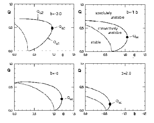
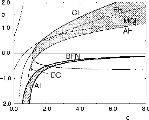

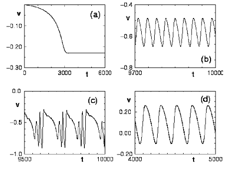

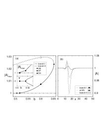
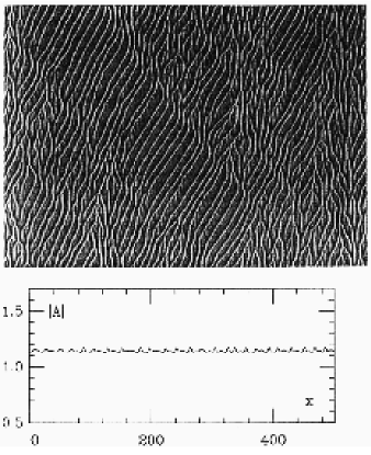
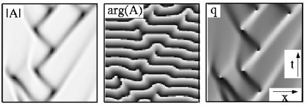
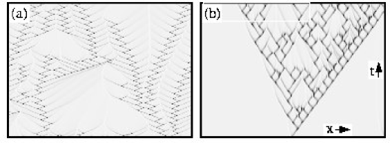
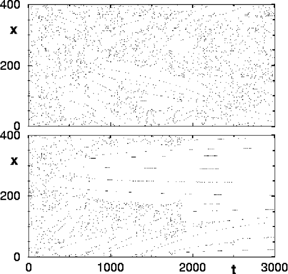
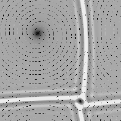
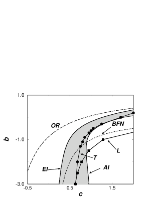

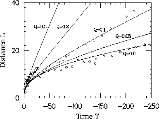
a) 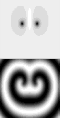 b)
b) 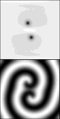
(a)  b)
b) 
(a)  b)
b) 

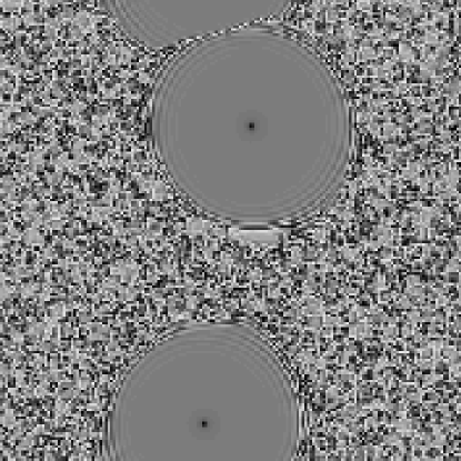
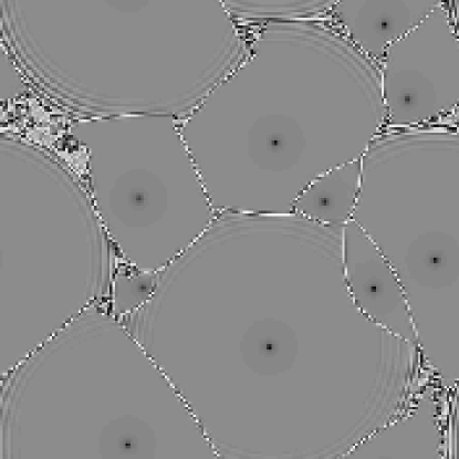

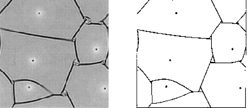
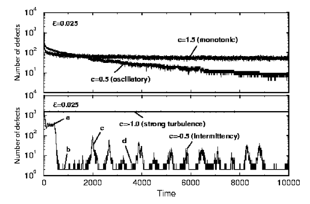
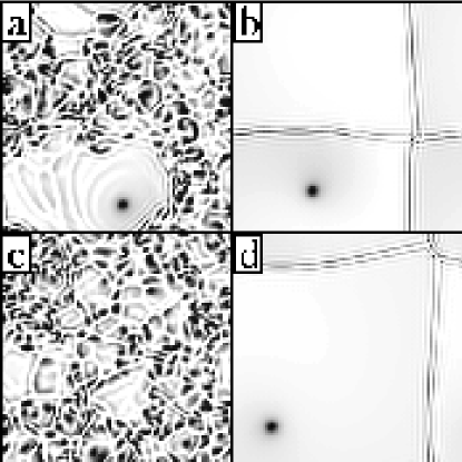
(a) 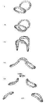 (b)
(b) 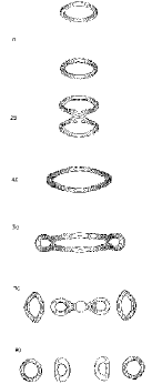
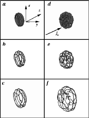

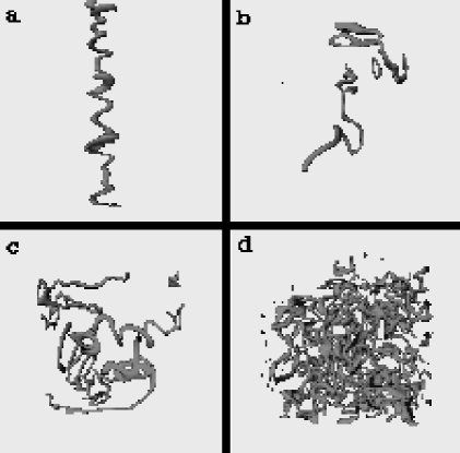

(a)  (b)
(b)