Two-loop renormalization-group analysis of critical behavior at $\boldsymbol{m}$-axial Lifshitz points

Abstract

We investigate the critical behavior that $d$-dimensional systems with short-range forces and a $n$-component order parameter exhibit at Lifshitz points whose wave-vector instability occurs in an $m$-dimensional isotropic subspace of ${\mathbb{R}}^{d}$. Utilizing dimensional regularization and minimal subtraction of poles in $d=4+{m\over 2}-\epsilon$ dimensions, we carry out a two-loop renormalization-group (RG) analysis of the field-theory models representing the corresponding universality classes. This gives the beta function $\beta_{u}(u)$ to third order, and the required renormalization factors as well as the associated RG exponent functions to second order, in $u$. The coefficients of these series are reduced to $m$-dependent expressions involving single integrals, which for general (not necessarily integer) values of $m\in(0,8)$ can be computed numerically, and for special values of $m$ analytically. The $\epsilon$ expansions of the critical exponents $\eta_{l2}$, $\eta_{l4}$, $\nu_{l2}$, $\nu_{l4}$, the wave-vector exponent $\beta_{q}$, and the correction-to-scaling exponent are obtained to order $\epsilon^{2}$. These are used to estimate their values for $d=3$. The obtained series expansions are shown to encompass both isotropic limits $m=0$ and $m=d$.

and

1 Introduction

The modern theory of critical phenomena [1, 2, 3] has taught us that the standard $|\boldsymbol{\phi}|^{4}$ models with a $n$-component order-parameter field $\boldsymbol{\phi}=(\phi_{i},\;i=1,\ldots,n)$ and $O(n)$ symmetric action have significance which extends far beyond the models themselves: They describe the long-distance physics of whole classes of microscopically distinct systems near their critical points. In fact, they are the simplest continuum models representing the $O(n)$ universality classes of $d$-dimensional systems with short-range interactions whose dimensions $d$ exceed the lower critical dimension $d_{*}$ ($=1$ or $2$) for the appearance of a transition to a phase with long-range order, and are less or equal than the upper critical dimension $d^{*}=4$ (above which Landau theory yields the correct asymptotic critical behavior). By investigating these models via sophisticated field theoretical methods [4], impressively accurate results have been obtained for universal quantities such as critical exponents and universal amplitude ratios.

A well-known crucial feature of these models is their scale (and conformal) invariance at criticality: The order-parameter density behaves under scale transformations asymptotically as

$$\boldsymbol{\phi}(\ell\boldsymbol{x})\sim\ell^{-x_{\phi}}\,\boldsymbol{\phi}(\boldsymbol{x})$$ (1)

in the infrared limit $\ell\to 0$, where $x_{\phi}=(d-2+\eta)/2$ is the scaling dimension of $\boldsymbol{\phi}$. This scale invariance is isotropic inasmuch as all $d$ coordinates of the position vector $\boldsymbol{x}$ are rescaled in the same fashion.

There exists, however, a wealth of phenomena that exhibit scale invariance of a more general, anisotropic nature. Roughly speaking, one can identify four different categories: (i) static critical behavior in anisotropic equilibrium systems such as dipolar-coupled uniaxial ferromagnets [5] or systems with Lifshitz points [6, 7], (ii) anisotropic critical behavior in stationary states of nonequilibrium systems (like those of driven diffusive systems [8] or encountered in stochastic surface growth [9]), (iii) dynamic critical phenomena of systems near thermal equilibrium [10], and (iv) dynamic critical phenomena in nonequilibrium systems [8].

In the cases of the first two categories, the coordinates $\boldsymbol{x}$ can be divided into two (or more) groups that scale in a different fashion. Writing $\boldsymbol{x}=({\boldsymbol{x}}_{\|},{\boldsymbol{x}}_{\perp})$, we call these parallel and perpendicular, respectively. Instead of Eq. (1) one then has

$$\boldsymbol{\phi}(\ell^{\theta}{\boldsymbol{x}}_{\|},\ell{\boldsymbol{x}}_{\perp})\sim\ell^{-x_{\phi}}\,\boldsymbol{\phi}({\boldsymbol{x}}_{\|},{\boldsymbol{x}}_{\perp})\;,$$ (2)

where $\theta$, the anisotropy exponent, differs from one. Categories (iii) and (iv) involve genuine time-dependent phenomena for which time typically scales with a nontrivial power of the length rescaling factor $\ell$. For phenomena of category (ii), one cannot normally avoid to deal also with the time evolution. This is because a fluctuation-dissipation theorem generically does not hold for such nonequilibrium systems; their stationary-state distributions are not fixed by given Hamiltonians of equilibrium systems and hence have to be determined from the long-time limit of their time-dependent distributions in general.

Category (i) provides very basic examples of systems exhibiting anisotropic scale invariance whose advantage is that they can be investigated entirely within the framework of equilibrium statistical mechanics. The particular example we shall be concerned with in this paper is the familiar continuum model for an $m$-axial Lifshitz point, defined by the Hamiltonian

$${\mathcal{H}}={\int}\!{d^{d}}x{\left\{{\rho_{0}\over 2}\,{({{\nabla}_{\parallel}}\boldsymbol{\phi})}^{2}+{\sigma_{0}\over 2}\,{(\triangle_{\|}\boldsymbol{\phi})}^{2}+\frac{1}{2}\,{({{\nabla}_{\perp}}\boldsymbol{\phi})}^{2}+{\tau_{0}\over 2}\,\boldsymbol{\phi}^{2}+\frac{u_{0}}{4!}\,|\boldsymbol{\phi}|^{4}\right\}}\;.$$ (3)

Here $\boldsymbol{\phi}(\boldsymbol{x})=(\phi_{i}(\boldsymbol{x}))_{i=1}^{n}$ is an $n$-component order-parameter field where $\boldsymbol{x}=(\boldsymbol{x}_{\|},\boldsymbol{x}_{\perp})\in{\mathbb{R}}^{m}\times{\mathbb{R}}^{d-m}$. The operators $\nabla_{\|}$, $\nabla_{\perp}$, and $\triangle_{\|}$ denote the $d_{\|}=m$ and $d_{\perp}=d{-}m$ dimensional parallel and perpendicular components of the gradient operator $\nabla$ and the associated Laplacian $\triangle_{\|}={\nabla_{\|}}^{2}$, respectively. The parameters $\sigma_{0}$ and $u_{0}$ are assumed to be positive. At zero-loop order (Landau theory), the Lifshitz point is located at $\rho_{0}=\tau_{0}=0$.

We recall that a Lifshitz point is a critical point where a disordered phase, a spatially uniform ordered phase, and a spatially modulated ordered phase meet. For further background and extensive lists of references, the reader is referred to review articles by Hornreich [6] and Selke [7] and to a number of more recent papers [11, 12, 13, 14, 15, 16, 17, 18].

An attractive feature of the model (3) is that the parameter $m$ can be varied. It was studied many years ago [19, 20, 21, 22] by means of an $\epsilon$ expansion about the upper critical dimension

$$d^{*}(m)=4+{m/2}\;,\quad m\leq 8\,.$$ (4)

The order-$\epsilon$ results for the correlation-length exponents $\nu_{l2}$ and $\nu_{l4}$, first derived by Hornreich et al. [19], are generally accepted. Yet long-standing controversies existed on the $\epsilon^{2}$ terms of the correlation exponents $\eta_{l2}$ and $\eta_{l4}$ and the wave-vector exponent $\beta_{q}$: Mukamel [20] gave results for all $m$ with $1\leq m\leq 8$. These agreed with what Hornreich and Bruce [21] found in the uniaxial case $m=1$ via an independent calculation, but were at variance with Sak and Grest’s [22] for $m=2$ and $m=6$ (who investigated only these special cases).

More recently, Mergulhão and Carneiro [13, 14] presented a reanalysis of the problem based on renormalized field theory and dimensional regularization. Treating explicitly only the cases $m=2$ and $m=6$, they recovered Sak and Grest’s results for $\eta_{l2}$ and $\eta_{l4}$, but did not compute $\beta_{q}$. They analytically continued in $d_{\|}$ rather than in $d_{\perp}$ and, fixing the latter at $d_{\perp}=4-{m/2}$ while taking the former as $d_{\|}=m-\epsilon_{\|}$, with $m=2$ or $6$, they also derived the expansions of the correlation-length exponents $\nu_{l2}$ and $\nu_{l4}$ to order $\epsilon_{\|}^{2}$.

The purpose of the present paper is to give a full two-loop renormalization group (RG) analysis of the model (3) for general, not necessarily integer values of $m\in(0,8)$ in $d=d^{*}(m)-\epsilon$ dimensions. As a result we obtain the $\epsilon$ expansions of all critical exponents $\eta_{l2}$, $\eta_{l4}$, $\beta_{q}$, $\nu_{l2}$, and $\nu_{l4}$ to order $\epsilon^{2}$. In a previous paper [18], hereafter referred to as I, we have shown how to overcome the severe technical difficulties that had hindered analytical progress in this field and prevented a resolution of the above-mentioned controversy for so long. Working directly in position space and exploiting the scale invariance of the free propagator at the Lifshitz point, we were able to compute the two-loop graphs of the two-point vertex function $\Gamma^{(2)}$ and $\Gamma^{(2)}_{(\nabla_{\|}\phi)^{2}}$, its analog with an insertion of ${\int}\!\d^{d}x\,{(\nabla_{\|}\phi)^{2}/2}$. Together with one-loop results, these suffice for determining the exponents $\eta_{l2}$, $\eta_{l4}$, and $\beta_{q}$ to order $\epsilon^{2}$. In order to obtain the correlation-length exponents $\nu_{l2}$ and $\nu_{l4}$ to this order in $\epsilon$ we must compute the two-loop graphs of the four-point vertex function $\Gamma^{(4)}$ and of $\Gamma^{(2)}_{\phi^{2}}$.

Our results are of importance to recent work on the generalization of conformal invariance to anisotropic scale invariant systems [25, 26, 27]. Some time ago Henkel [25] proposed a new set of infinitesimal transformations generalizing scale invariance for systems of this kind with an anisotropy exponent $\theta=2/\wp$, $\wp=1,2,\ldots$. He pointed out that the case $\wp=4$, $\theta=1/2$, is realized for the Lifshitz point of a spherical ($n\to\infty$) analog of the ANNNI model [28, 29], and that the same $m$-independent value of $\theta$ in Ref.  [28] was found to persist to first order in $\epsilon$ for the Lifshitz point of the model (3). However, as can be seen from Eq. (66) below [and Eq. (84) of I], $\theta$ deviates from $1/2$ at order $\epsilon^{2}$. This shows that the Lie algebra discussed in Ref. [25] cannot strictly apply below the upper critical dimension ($\epsilon>0$) if $n$ is finite, except in the trivial Gaussian case $u_{0}=0$.

The remainder of this paper is organized as follows. In the next section we recapitulate the scaling form of the free propagator for $\tau_{0}=\rho_{0}=0$. We give the explicit form of its scaling function as well as those of similar quantities, and discuss their asymptotic behavior for large values of their argument. These informations are required in the sequel since the expansion coefficients of our results for the renormalization factors and critical exponents can be expressed in terms of single integrals involving these functions.

In Sec. 3 we specify our renormalization procedure and present our two-loop results for the renormalization factors. Our $\epsilon$-expansion results for the critical, correction-to-scaling, and crossover exponents are described in Sec.  4. Utilizing these we determine numerical estimates for the values of these exponents in $d=3$ dimensions, which we compare with available results from Monte Carlo calculations and other sources. Section 5 contains a brief summary and concluding remarks. In the Appendixes A–E various calculational details are described.

2 Scaling functions of the free theory and their asymptotic behavior

2.1 The free propagator and its scaling function

Following the strategy utilized in I, we employ in our perturbative renormalization scheme the free propagator with $\tau_{0}=\rho_{0}=0$. In position space, it is given by

$$G({\boldsymbol{x}})=G(x_{\|},x_{\perp})=\int_{\boldsymbol{q}}{\e^{i{\boldsymbol{q}}\cdot{\boldsymbol{x}}}\over q_{\perp}^{2}+\sigma_{0}{q_{\|}^{4}}}\,.$$ (5)

Here $x_{\|}=|{\boldsymbol{x}}_{\|}|$ and $x_{\perp}=|{\boldsymbol{x}}_{\perp}|$ are the Euclidean lengths of the parallel and perpendicular components of ${\boldsymbol{x}}$, and we have introduced the notation

$$\int_{\boldsymbol{q}}\equiv\int_{{\boldsymbol{q}}_{\|}}\int_{{\boldsymbol{q}}_{\perp}}\;\quad\mbox{with}\quad\int_{{\boldsymbol{q}}_{\|}}\equiv{\int_{{\mathbb{R}}^{m}}}{\d^{m}q_{\|}\over(2\pi)^{m}}\quad\quad\mbox{and}\quad\int_{{\boldsymbol{q}}_{\perp}}\equiv{\int_{{\mathbb{R}}^{d-m}}}{\d^{d-m}q_{\perp}\over(2\pi)^{d-m}}\;$$ (6)

for integrals over momenta $\boldsymbol{q}=({\boldsymbol{q}}_{\|},{\boldsymbol{q}}_{\perp})\in\Rset^{m}\times\Rset^{d-m}$. Whenever necessary, these integrals are dimensionally regularized.

Rescaling the momenta as ${{\boldsymbol{q}}_{\|}}\sigma_{0}^{1/4}\sqrt{x_{\perp}}\to{\boldsymbol{q}}_{\|}$ and ${{\boldsymbol{q}}_{\perp}}x_{\perp}\to{\boldsymbol{q}}_{\perp}$ yields the scaling form [18] (cf. Ref. [25, 29])

$$G(x_{\|},x_{\perp})=x_{\perp}^{-2+\epsilon}\,\sigma_{0}^{-{m/4}}\,{\Phi}{\left({\sigma_{0}^{-{1/4}}\,{x_{\|}}\,x_{\perp}^{-1/2}}\right)}$$ (7)

with the scaling function

$$\Phi(\upsilon)\equiv\Phi(\upsilon;m,d)=\int_{{\boldsymbol{q}}_{\|}}\int_{{\boldsymbol{q}}_{\perp}}{\e^{i{{\boldsymbol{q}}_{\perp}}\cdot{\boldsymbol{e}}_{\perp}}\,\e^{i{\boldsymbol{q}}_{\|}\cdot\boldsymbol{\upsilon}}\over q_{\perp}^{2}+q_{\|}^{4}}\,,$$ (8)

where ${\boldsymbol{e}}_{\perp}$ is an arbitrary unit $d_{\perp}$-vector while $\boldsymbol{\upsilon}$ stands for the dimensionless $d_{\|}$-vector

$$\boldsymbol{\upsilon}=\sigma_{0}^{-{1/4}}\,{\boldsymbol{x}}_{\|}\,x_{\perp}^{-1/2}\,.$$ (9)

In I the following representation of $\Phi(\upsilon)$ in terms of generalized hypergeometric functions was obtained:

$${\Phi}(\upsilon) = \,2^{-2-m}\,\pi^{-{d-1\over 2}}\,\hat{\Phi}(\upsilon)\;,$$ (10)

$$\hat{\Phi}(\upsilon) = {\Gamma{\left(1{-}{\epsilon\over 2}\right)}\over\Gamma{\left({1\over 2}{+}{m\over 4}\right)}}\;{\mathop{{}_{1\!}{F}_{2\!}}\nolimits}{\left(1{-}{\epsilon\over 2};{1\over 2},{1\over 2}{+}{m\over 4};{\upsilon^{4}\over 64}\right)}$$ (11)

$$\mbox{}-{\upsilon^{2}\over 4}{\Gamma{\left({3\over 2}{-}{\epsilon\over 2}\right)}\over\Gamma{\left(1{+}{m\over 4}\right)}}\;{\mathop{{}_{1\!}{F}_{2\!}}\nolimits}{\left({3\over 2}{-}{\epsilon\over 2};{3\over 2},1{+}{m\over 4};{\upsilon^{4}\over 64}\right)}\,,$$

with $\epsilon=4+\frac{m}{2}-d$. Upon expanding the hypergeometric functions in powers of $\upsilon^{4}$ and resumming, one arrives at the Taylor expansion

$$\hat{\Phi}(\upsilon)=\sum_{k=0}^{\infty}{1\over k!}\,{\Gamma{\left(1-{\epsilon\over 2}+{k\over 2}\right)}\over\Gamma{\left({1\over 2}+{m\over 4}+{k\over 2}\right)}}\,{\left(-{\upsilon^{2}\over 4}\right)}^{k}\;.$$ (12)

The result tells us that $\hat{\Phi}$ can be written in the form

$$\hat{\Phi}(\upsilon)={{}_{1}\!\Psi_{1}}{\left[{\left(1{-}{\epsilon\over 2},{1\over 2}\right)};{\left(\frac{1}{2}{+}\frac{m}{4},\frac{1}{2}\right)};-{\upsilon^{2}\over 4}\right]}\;,$$ (13)

where ${{}_{1}\!\Psi_{1}}$ is a particular one of the Fox-Wright $\Psi$ functions (or Wright functions) ${{}_{p}\!\Psi_{q}}$ [30, 31, 32, 33, 34], further generalizations of the generalized hypergeometric functions $\mathop{{}_{p}{F}_{q\!}}\nolimits$ whose series representations are given by

$${\mathop{{}_{p\!}\Psi_{q}}\nolimits}[\{(a_{i},A_{i})\},\{(b_{j},B_{j}\};x]=\sum_{k=0}^{\infty}{1\over k!}\;{\prod_{i=1}^{p}\Gamma(a_{i}+A_{i}\,k)\over\prod_{i=1}^{q}\Gamma(b_{j}+B_{j}\,k)}\;x^{k}\;.$$ (14)

In the sequel, we shall need the asymptotic behavior of $\Phi(\upsilon)$ as $\upsilon\to\infty$. This may be inferred from theorems due to Wright [31, 32] about the asymptotic expansions of the functions $\mathop{{}_{p\!}\Psi_{q}}\nolimits$. We discuss this matter in Appendix A, where we show that the asymptotic expansion these theorems predict for nonexceptional values of $m$ and $\epsilon$,

$$\hat{\Phi}(\upsilon\to\infty)\approx{\left({\upsilon\over 2}\right)}^{-4+2\epsilon}\sum_{k=0}^{\infty}{(-1)^{k}\over k!}\,{2\,\Gamma(2-\epsilon+2k)\over\Gamma({m\over 4}{-}{1\over 2}{+}{\epsilon\over 2}{-}k)}\,{\left({\upsilon\over 2}\right)}^{-4k}\;,$$ (15)

follows from the integral representation (8) in an equally straightforward manner as the Taylor expansion (12). Nonexceptional values of $m$ and $\epsilon$ are characterized by the property that none of the poles which the nominator of the coefficient

$$f(k)={\Gamma{\left(1-{\epsilon\over 2}+{k\over 2}\right)}\over\Gamma{\left({1\over 2}+{m\over 4}+{k\over 2}\right)}}$$ (16)

of the power series (12) has at

$$k=k_{l}\equiv\epsilon-2\,l\;,\quad l=1,2,\ldots,$$ (17)

gets canceled by a pole of the denominator. If $\epsilon=0$, the only values among $m=1,2,\ldots,7$ for which such cancellations occur are $m=2$ and $m=6$. More generally, this happens for $d=m+1$ and $d=m+3$ where the expansion (15) terminates after the first ($k=0$) term and vanishes identically, respectively. In accordance with Wright’s theorems, corrections to these truncated expansions are exponentially small. In fact, in these two cases $\Phi(\upsilon)$ reduces to the much simpler expressions

$$\Phi(\upsilon)={u^{2-m}\over 8\,{\pi}^{m/2}}\;{\gamma}{\left(\frac{m-2}{2},\frac{\upsilon^{2}}{4}\right)}\;,\qquad d=m+1\,,$$ (18)

and

$$\Phi(\upsilon)={(4\,\pi)^{-{m+2\over 2}}}\,\e^{-{\upsilon^{2}/4}}\;,\qquad d=m+3\,,$$ (19)

where $\gamma(a,x)$ is the incomplete gamma function. These equations comprise two cases where $d$ becomes the upper critical dimension (4), namely $(d,m)=(6,7)$ and $(d,m)=(2,5)$. In the former, Eq. (18) simplifies to

$$\Phi(\upsilon)={1\over(2\pi)^{3}}\,{1\over\upsilon^{4}}\,{\left[1-{\left(1+{\upsilon^{2}\over 4}\right)}\,{\e}^{-{\upsilon^{2}/4}}\right]}\;,\quad m=6\,,\;d=d^{*}=7\,.$$ (20)

This result as well as Eq. (19) with $m=2$ were employed in I, where we also derived the leading term ($k=0$) of the asymptotic series (15).

For general values of $m$ and $d=d^{*}$, the scaling function $\Phi(\upsilon;m,d)\equiv\Phi(\upsilon)$ can be written as

$${\Phi}(\upsilon;m,d^{*})=\frac{1}{2^{2+m}\,\pi^{\frac{6{+}m}{4}}}\,{\left[{{\mathop{{}_{1\!}{F}_{2\!}}\nolimits}{\left(1;{1\over 2},{2{+}m\over 4};{\upsilon^{4}\over 64}\right)}\over\Gamma{\left({2{+}m\over 4}\right)}}-\sqrt{\pi}\,{\left({{\upsilon}^{2}\over 8}\right)}^{1{-}{m\over 4}}\;{{I}_{m\over 4}}{\left({\upsilon^{2}\over 4}\right)}\right]}$$

$$=\frac{1}{2^{2+m}\,\pi^{\frac{6{+}m}{4}}}\,{\left\{\frac{1}{\Gamma{\left(\frac{2+m}{4}\right)}}+\sqrt{\pi}\,{\left({{\upsilon}^{2}\over 8}\right)}^{1{-}{m\over 4}}{\left[{\mathop{\mathbf{L}}\nolimits}_{\frac{m}{4}}{\left({\upsilon^{2}\over 4}\right)}-{{I}_{m\over 4}}{\left({\upsilon^{2}\over 4}\right)}\right]}\right\}},$$

where $\mathop{\mathbf{L}}\nolimits_{\alpha}(z)$ and $I_{\alpha}(z)$ are modified Struve and Bessel functions, respectively [35].

The second form is in conformity with the one given by Frachebourg and Henkel [29] for the case $m=1$. These authors encountered this (and similar) scaling functions when studying Lifshitz points of order $L-1$ of spherical models. They also analyzed the large-$\upsilon$ behavior of these functions, verifying explicitly the asymptotic forms predicted by Wright’s theorems. If we let $a=1$ and set $x=\upsilon^{2}/4$, their scaling function denoted $\Psi(a,x)$ corresponds precisely to our $\hat{\Phi}(\upsilon)$, and the asymptotic expansion they found is consistent with ours in Eq. (15) and the large-$\upsilon$ form (22) presented below.

Finally, let us explicitly give the large-$\upsilon$ forms of $\Phi(\upsilon,m,d^{*})$ as implied by Eq. (15):

$$\Phi(\upsilon;m,d^{*}) \mathop{\approx}\limits_{\upsilon\to\infty} 2^{1-m}\,\pi^{-{6+m\over 4}}\,{m-2\over\Gamma({m+2\over 4})}{\left[{1\over\upsilon^{4}}-{24\,(m-6)\over\upsilon^{8}}\right.}$$ (22)

$${\qquad\qquad\qquad\left.\mbox{}+{960\,(m-10)(m-6)\over\upsilon^{12}}+O{\left(\upsilon^{-16}\right)}\right]}.$$

In accordance with our previous considerations, all terms or all but the first one of this series vanish when $m=2$ or $m=6$, respectively.

2.2 Other required scaling functions of the free theory

Besides $\Phi$, our results to be given below involve two other scaling functions. One is the function $\Xi(\upsilon;m,d)$ of I. This is defined through

$$-(\nabla_{\|}G*{\nabla_{\|}}G)(\boldsymbol{x})=x_{\perp}^{-1+\epsilon}\,\sigma_{0}^{-(m+2)/4}\,\Xi\big{(}\sigma_{0}^{-1/4}x_{\parallel}x_{\perp}^{-1/2}\big{)}\,,$$ (23)

where the asterisk indicates a convolution, i.e., $(f{*}g)({\boldsymbol{x}})\equiv{\int}\d^{d}x^{\prime}\,f({\boldsymbol{x}}-{\boldsymbol{x}}^{\prime})\,g({\boldsymbol{x}}^{\prime})$. The explicit form of $\Xi(\upsilon;m,d^{*})$ may be gleaned from Eq. (A5) of I, where it was given in terms of Bessel and hypergeometric functions. This can be written more compactly as

$$\Xi(\upsilon;m,d^{*})=\frac{{\upsilon}^{2{-}{m\over 2}}}{2^{6+\frac{m}{4}}\,\pi^{\frac{4{+}m}{4}}}\,{\left[{I}_{\frac{m-4}{4}}{\left({\upsilon^{2}\over 4}\right)}-{{\mathop{\mathbf{L}}\nolimits}_{m-4\over 4}}{\left({\upsilon^{2}\over 4}\right)}\right]}\;.$$ (24)

The asymptotic expansion of the difference of functions in the square brackets of this equations follows from Eqs. (12.2.6) and (9.7.1) of Ref. [35], implying

$$\Xi(\upsilon;m,d^{*}) \mathop{\approx}\limits_{\upsilon\to\infty} 2^{-2-m}\,\pi^{-\frac{6+m}{4}}{m-2\over\Gamma{\left(\frac{m+2}{4}\right)}}\,\upsilon^{-2}\,{\left[1+{6-m\over 2}\,{4^{2}\over\upsilon^{4}}\right.}$$ (25)

$$\mbox{}+{\left.{6-m\over 2}\,{3\,(10-m)\over 2}\,{4^{4}\over\upsilon^{8}}+O{\left(\upsilon^{-12}\right)}\right]}\;.$$

The leading term $\sim\upsilon^{-2}$ was already given in I. Note also that again all terms or all but the first one of this series vanish when $m=2$ or $m=6$, respectively, as is borne out by the explicit forms

$$\Xi(\upsilon;2,5)=\frac{1}{2}\,\Phi(\upsilon;2,5)=\frac{\e^{-\upsilon^{2}/4}}{32\,\pi^{2}}$$ (26)

and

$$\Xi(\upsilon;6,7)={1-\e^{-\upsilon^{2}/4}\over(4\,\pi)^{3}\,\upsilon^{2}}\;.$$ (27)

The third scaling function we shall need is defined through the Taylor expansion

$$\Theta(\upsilon;m)\equiv\sum_{k=1}^{\infty}{\Gamma{\left({k\over 2}\right)}\over k!\;\Gamma{\left({1\over 2}{+}{m\over 4}{+}{k\over 2}\right)}}\,{\left({-\upsilon^{2}\over 4}\right)}^{k}\;.$$ (28)

It can be expressed in terms of generalized hypergeometric functions $\mathop{{}_{p}{F}_{q\!}}\nolimits$ by summing the contributions with even and odd $k$ separately. One finds

$$\Theta(\upsilon;m) = {\upsilon^{4}\over 32}\,{1\over\Gamma({3\over 2}{+}{m\over 4})}\,\mathop{{}_{2}{F}_{3\!}}\nolimits{\left(1,1;{3\over 2},2,{3\over 2}{+}{m\over 4};{\upsilon^{4}\over 64}\right)}$$ (29)

$$\mbox{}-{\upsilon^{2}\over 4}{\sqrt{\pi}\over\Gamma(1{+}{m\over 4})}\;\mathop{{}_{1\!}{F}_{2\!}}\nolimits{\left({1\over 2};{3\over 2},1{+}{m\over 4};{\upsilon^{4}\over 64}\right)}\;.$$

Details of how this function arises in the computation of the Laurent expansion of the four-point graph pt 1.5 0.3 (-7 -1.5)(15 6) (-7 1.5)(15 -6) (5 0) rx:1 ry:3 may be found in Appendix C. In Appendix D we show that $\Theta(\upsilon,m)$ behaves as

$$\Theta(\upsilon;m) \mathop{\approx}\limits_{\upsilon\to\infty} {1\over\Gamma{\left({2+m\over 4}\right)}}\,{\left[-\ln{\upsilon^{4}\over 16}+\psi{\left({m+2\over 4}\right)}-C_{E}-8\,\frac{m-2}{\upsilon^{4}}\right.}$$ (30)

$$\qquad\qquad\qquad{\left.\mbox{}+96\,\frac{(m-2)(m-6)}{\upsilon^{8}}\right]}+O{\left(\upsilon^{-12}\right)}$$

in the large-$\upsilon$ limit, where $C_{E}\simeq 0.577216$ is Euler’s constant and while $\psi(x)$ denotes the digamma function.

For the special values $m=2$ and $m=6$, the function $\Theta(\upsilon;m)$ reduces to a sum of elementary functions and the exponential integral function $E_{1}(x)$. As can be easily deduced from the series expansion (28), one has

$$\Theta(\upsilon,2)=-2\,{\left[C_{E}+\ln{\upsilon^{2}\over 4}+E_{1}{\left({\upsilon^{2}\over 4}\right)}\right]}$$ (31)

and

$$\Theta(\upsilon,6) = 1-2\,C_{E}-\ln{\upsilon^{4}\over 16}-2\,E_{1}{\left({\upsilon^{2}\over 4}\right)}+\frac{8\,\e^{-{\upsilon^{2}/4}}}{\upsilon^{2}}+32\,\frac{\e^{-{\upsilon^{2}/4}}-1}{\upsilon^{4}}$$ (32)

$$= 1+\Theta(\upsilon;2)-\hat{\Phi}(\upsilon;6,7)\;,$$

respectively.

3 Renormalization

3.1 Reparametrizations

¿From I we know that the ultraviolet singularities of the $N$-point correlation functions $\langle{\prod_{\nu=1}^{N}}\phi_{i_{\nu}}({\boldsymbol{x}}_{\nu})\rangle$ of the Hamiltonian (3) can be absorbed via reparametrizations of the form

$$\phi={Z_{\phi}}^{{1}/{2}}\,\phi_{\mathrm{ren}}\;,$$ (33)

$$\tau_{0}-\tau_{0c}=\mu^{2}\,Z_{\tau}\,\tau\;,$$ (34)

$$\sigma_{0}=Z_{\sigma}\,\sigma\;,$$ (35)

$$u_{0}\,{\sigma_{0}}^{-m/4}\,F_{m,\epsilon}=\mu^{\epsilon}\,Z_{u}\,u\;,$$ (36)

and

$$\left(\rho_{0}-\rho_{0c}\right)\,{\sigma_{0}}^{-1/2}=\mu\,Z_{\rho}\,\rho\;.$$ (37)

Here $\mu$ is an arbitrary momentum scale. The critical values of the Lifshitz point, $\sigma_{0c}$ and $\rho_{0c}$, vanish in our perturbative RG scheme based on dimensional regularization and the $\epsilon$ expansion. The factor $F_{m,\epsilon}$ serves to choose a convenient normalization of $u$. A useful choice is to write the following one-loop integral for pt 2.5 0.3 rx:4 ry:1.8 (4 0)(2 2) (4 0)(2 -2) (-4 0)(-2 -2) (-4 0)(-2 2) as

$${\int_{\boldsymbol{q}}}{1\over(q_{\|}^{4}+q_{\perp}^{2})[q_{\|}^{4}+({\boldsymbol{q}}_{\perp}+{\boldsymbol{e}}_{\perp})^{2}]}=\frac{F_{m,\epsilon}}{\epsilon}\;.$$ (38)

This integral is evaluated in Appendix C. The result, given in Eq. (119), yields

$$F_{m,\epsilon} = (4\,\pi)^{-{8+m-2\,\epsilon\over 4}}\,\frac{\Gamma{\left(1+{\epsilon\over 2}\right)}\,\Gamma^{2}{\left(1-{\epsilon\over 2}\right)}\,\Gamma{\left(\frac{m}{4}\right)}}{\Gamma(2-\epsilon)\,\Gamma{\left(\frac{m}{2}\right)}}$$ (39)

$$= \frac{(4\,\pi)^{-2-\frac{m}{4}}\,\Gamma(\frac{m}{4})}{\Gamma(\frac{m}{2})}\,{\left[1+(2-C_{E}+\ln 4\pi)\,{\epsilon\over 2}+O(\epsilon^{2})\right]}\;.$$

3.2 Renormalization factors

With this different choice of normalization of the coupling constant, our results of I for $Z_{\phi}$, $Z_{\sigma}$, and $Z_{\rho}$ translate into

$$Z_{\phi}=1-\frac{n{+}2}{3}\,\frac{j_{\phi}(m)}{12\,(8-m)}\,\frac{u^{2}}{\epsilon}+O(u^{3})\;,$$ (40)

$${Z_{\sigma}}Z_{\phi}=1+\frac{n{+}2}{3}\,{j_{\sigma}(m)\over 96\,m(m{+}2)}\,\frac{u^{2}}{\epsilon}+O(u^{3})\;,$$ (41)

and

$${Z_{\rho}}{Z_{\phi}}{Z_{\sigma}^{1/2}}=1+\frac{n{+}2}{3}\,{j_{\rho}(m)\over 8\,m}\,\frac{u^{2}}{\epsilon}+O(u^{3})$$ (42)

with

$$j_{\phi}(m)\equiv B_{m}\,{\int_{0}^{\infty}}\!{\d}\upsilon\,\upsilon^{m-1}\,\Phi^{3}(\upsilon;m,d^{*})\;,$$ (43)

$$j_{\sigma}(m)\equiv B_{m}\,{\int_{0}^{\infty}}\!{\d}\upsilon\,\upsilon^{m+3}\,\Phi^{3}(\upsilon;m,d^{*})\;,$$ (44)

and

$$j_{\rho}(m)\equiv B_{m}\,{\int_{0}^{\infty}}\!{\d}\upsilon\,\upsilon^{m+1}\,\Phi^{2}(\upsilon;m,d^{*})\,\Xi(\upsilon;m,d^{*})\;.$$ (45)

Except for the factor $B_{m}$, which is

$$B_{m}\equiv\frac{S_{4-{m\over 2}}\,S_{m}}{F_{m,0}^{2}}={\frac{{2^{10+m}}\,{{\pi}^{6+{\frac{3\,m}{4}}}}\,\Gamma({\frac{m}{2}})}{\Gamma(2-{\frac{m}{4}})\,{{\Gamma({\frac{m}{4}})}^{2}}}}\;,$$ (46)

the coefficients $j_{\phi}(m)$, $j_{\sigma}(m)$, and $j_{\rho}(m)$ are precisely the integrals denoted respectively as $J_{0,3}(m,d^{*})$, $J_{4,3}(m,d^{*})$, and $I_{1}(m,d^{*})$, in I. The quantity $S_{d}=2\,\pi^{d/2}/\Gamma(d/2)$ in Eq. (46) (with $d=m$, e.g.) means the surface area of a $d$-dimensional unit sphere.

Our two-loop results for the remaining $Z$-factors, $Z_{u}$ and $Z_{\tau}$, can be written as

$${Z_{\tau}}Z_{\phi}=1+\frac{n{+}2}{3}\,\frac{u}{2\,\epsilon}+\frac{n{+}2}{3}{\left[\frac{n{+}5}{6}\,\frac{1}{\epsilon^{2}}-{J_{u}(m)\over 2\,\epsilon}\right]}\,{u^{2}\over 2}+O(u^{3})$$ (47)

and

$${Z_{u}}{Z_{\phi}^{2}}{Z_{\sigma}^{m/4}} = 1+\frac{n{+}8}{9}\,\frac{3\,u}{2\,\epsilon}+{\left[{\left(\frac{n{+}8}{9}\,{3\over 2\,\epsilon}\right)}^{2}-3\,{5n{+}22\over 27}\,{J_{u}(m)\over 2\,\epsilon}\right]}\,u^{2}$$ (48)

$$\mbox{}+O(u^{3})\;,$$

with

$$J_{u}(m)=1-{C_{E}+\psi{\left(2-\frac{m}{4}\right)}\over 2}+j_{u}(m)\;,$$ (49)

where $j_{u}(m)$ means the integral

$$j_{u}(m)=\frac{B_{m}}{2^{4+m}\,\pi^{(6+m)/4}}\,{\int_{0}^{\infty}}\d\upsilon\,\upsilon^{m-1}\,\Phi^{2}(\upsilon;m,d^{*})\,\Theta(\upsilon;m)\;.$$ (50)

For the values $m=2$ and $m=6$, the above integrals $j_{\phi}$, $j_{\sigma}$, $j_{\rho}$, and $j_{u}$ can be computed analytically (cf. I and Appendices B and C). This gives

$$j_{\phi}(2)=\frac{4}{3}\;,\qquad j_{\phi}(6)=\frac{8}{3}\,{\left[1-3\,\ln{4\over 3}\right]}\;,$$ (51)

$$j_{\sigma}(2)=\frac{128}{27}\;,\qquad j_{\sigma}(6)=\frac{448}{9}\;,$$ (52)

$$j_{\rho}(2)=\frac{8}{9}\;,\qquad j_{\rho}(6)=\frac{8}{3}\,{\left[1+6\ln{4\over 3}\right]}\;,$$ (53)

$$j_{u}(2)=-\ln\frac{3}{2}\;,\qquad j_{u}(6)=-{\left(\frac{1}{6}+\ln{128\over 27}\right)}\;,$$ (54)

and

$$J_{u}(2)=\ln\frac{4}{3}\;,\qquad J_{u}(6)=\frac{5}{6}-3\,\ln\frac{4}{3}\;.$$ (55)

For other values of $m$ we determined these integrals by numerical integration in the manner explained in Appendix E. The results are listed in Table 1.

Table 1: Numerical values of the integrals $j_{\phi}(m)$, …, $J_{u}(m)$.

m	1	2	3	4	5	6	7
$j_{\phi}$	1.642(9)	1.33333	1.055(6)	0.803(7)	0.57(4)	0.36521	0.17(4)
$j_{\sigma}$	1.339(4)	4.74074	10.804(3)	20.067(7)	32.95(4)	49.77778	70.74(7)
$j_{\rho}$	0.190(6)	0.88889	1.999(9)	3.464(1)	5.23(4)	7.26958	9.53(6)
$j_{u}$	-0.203(7)	-0.40547	-0.624(2)	-0.880(1)	-1.21(1)	-1.72286	-2.92(4)
$J_{u}$	0.383(8)	0.28768	0.200(8)	0.119(8)	0.04(3)	-0.02971	-0.09(9)

3.3 Beta function and fixed-point value $u^{*}$

¿From the above results for the renormalization factors the beta function

$$\beta_{u}(u)\equiv{\left.\mu\partial_{\mu}\right|_{0}}\,u$$ (56)

and the exponent functions

$$\eta_{\iota}\equiv{\left.\mu\partial_{\mu}\right|_{0}}\,\ln Z_{\iota}\,,\quad\iota=\phi,\,\sigma,\,\rho,\,\tau,\,u,$$ (57)

can be calculated in a straightforward manner. Here ${\left.\partial_{\mu}\right|_{0}}$ denotes a derivative at fixed bare values $\sigma_{0}$, $\tau_{0}$, $\rho_{0}$, and $u_{0}$. Since we employed minimal subtraction of poles, the exponent functions satisfy the following simple relationship to the residua ($\mathop{\mathrm{Res}}\nolimits$) of the $Z$ factors:

$$\eta_{\iota}(u)=-u\partial_{u}\mathop{\mathrm{Res}}\nolimits_{\epsilon=0}[Z_{\iota}(u)]\;,\quad\iota=\phi,\,\sigma,\,\rho,\,\tau,\,u.$$ (58)

For the beta function, which is related to $\eta_{u}$ via $\beta_{u}(u)=-u[\epsilon+\eta_{u}(u)]$, we obtain

$$\beta_{u}(u) = -\epsilon\,u+\frac{n{+}8}{9}\,\frac{3}{2}\,u^{2}-{\Bigg{\{}3\,{5n{+}22\over 27}\,J_{u}(m)}$$ (59)

$$\mbox{}+{\left.\frac{1}{24}\,\frac{n{+}2}{3}{\left[{j_{\sigma}(m)\over 8\,(m{+}2)}-j_{\phi}(m)\right]}\right\}}\,u^{3}+O(u^{4})\;.$$

Upon solving for the nontrivial zero of $\beta_{u}$, we see that the infrared-stable fixed point is located at

$$u^{*} = \frac{2\,\epsilon}{3}\,\frac{9}{n{+}8}+\frac{8\,\epsilon^{2}}{27}\,{\left(\frac{9}{n{+}8}\right)}^{3}\,{\Bigg{\{}3\,{5n{+}22\over 27}\,J_{u}(m)}$$ (60)

$$\qquad\qquad\quad\mbox{}+{\left.\frac{1}{24}\,\frac{n{+}2}{3}\,{\left[{j_{\sigma}(m)\over 8\,(m{+}2)}-j_{\phi}(m)\right]}\right\}}+O{(\epsilon^{3})}\;.$$

We refrain from giving the resulting lengthy expressions for the exponent functions here. The values $\eta_{\iota}^{*}\equiv\eta_{\iota}(u^{*})$ of these functions at the infrared-stable fixed point are presented in Eqs. (61)–(66) below.

4 Critical exponents

4.1 Analytic $\epsilon$-expansion results

The fixed-point value (60) can now be substituted into the exponent functions (58) that are implied by our results (40)–(42) and (47) for the renormalization factors to obtain the universal quantities $\eta_{\iota}^{*}=\eta_{\iota}(u^{*})$, $\iota=\phi$, $\sigma$, $\rho$, and $\tau$. Recalling how these are related to the critical exponents (cf. I), one arrives at the $\epsilon$ expansions

$$\eta_{l2}=\eta_{\phi}^{*}=\frac{n+2}{(n+8)^{2}}\,\frac{2\,j_{\phi}(m)}{8-m}\,\epsilon^{2}+O(\epsilon^{3})\;,$$ (61)

$$\eta_{l4}=4\,\frac{\eta_{\phi}^{*}+\eta_{\sigma}^{*}}{2+\eta_{\sigma}^{*}}=-\frac{n+2}{(n+8)^{2}}\,\frac{j_{\sigma}(m)}{2m\,(m+2)}\,\epsilon^{2}+O(\epsilon^{3})\;,$$ (62)

$${1\over\nu_{l2}}-2=\eta_{\tau}^{*} = -{n{+}2\over n{+}8}\,{\epsilon}-{n{+}2\over 2\,(n{+}8)^{2}}\Bigg{\{}4\,{7n{+}20\over n{+}8}J_{u}(m)+{n{+}2\over n{+}8}\,{j_{\sigma}(m)\over 8\,(m{+}2)}$$ (63)

$$\mbox{}+{m\,(n{+}2)+4\,(4{-}n)\over(n{+}8)(8{-}m)}\,j_{\phi}(m)\Bigg{\}}\epsilon^{2}+O(\epsilon^{3})\,,$$

$$\nu_{l4}=\frac{2+\eta_{\sigma}^{*}}{4\,(2+\eta_{\tau}^{*})} = \frac{1}{4}+{n{+}2\over n{+}8}\,{\epsilon\over 8}+{1\over 16}\,{n+2\over(n{+}8)^{2}}\Bigg{\{}n{+}2+4\,\frac{7n{+}20}{n{+}8}\,J_{u}(m)$$

$${\mbox{}-{n{+}2\over n{+}8}\,j_{\phi}(m)-{\left[1-{m\over 4}\,{n{+}2\over n{+}8}\right]}\,{j_{\sigma}(m)\over 2m(m{+}2)}\Bigg{\}}}\epsilon^{2}+O(\epsilon^{3})\;,$$

and

$${\varphi\over\nu_{l2}}-1=\eta_{\rho}^{*}={n+2\over(n+8)^{2}}\,{\left[{j_{\sigma}(m)\over 8\,m\,(m{+}2)}-\frac{3\,j_{\rho}(m)}{m}-\frac{j_{\phi}(m)}{8{-}m}\right]}\,\epsilon^{2}+O(\epsilon^{3})\,.$$ (65)

The anisotropy exponent $\theta={\nu_{l4}/\nu_{l2}}$ of Eq. (2) is given by

$$\theta=\frac{2+\eta_{\sigma}^{*}}{4}=\frac{1}{2}-\frac{n+2}{2\,(n+8)^{2}}\,{\left[{j_{\sigma}(m)\over 8\,m\,(m+2)}+{j_{\phi}(m)\over 8-m}\right]}\,\epsilon^{2}+O(\epsilon^{3})\;,$$ (66)

and for the correction-to-scaling exponent, we obtain

$$\omega_{l2}\equiv\beta_{u}^{\prime}(u^{*}) = \epsilon-\frac{36\,\epsilon^{2}}{(n+8)^{2}}\,{\left\{3\,{5n{+}22\over 27}\,J_{u}(m)\right.}$$ (67)

$$\qquad\qquad\mbox{}+{\left.\frac{1}{24}\,\frac{n{+}2}{3}{\left[{j_{\sigma}(m)\over 8\,(m{+}2)}-j_{\phi}(m)\right]}\right\}}+O(\epsilon^{3})\;.$$

Our rationale for denoting the latter analog of the usual Wegner exponent as $\omega_{l2}$ is the following: It governs those corrections to scaling that are weaker by a factor of $\xi_{\perp}^{-\omega_{l2}}\sim|\tau|^{\nu_{l2}\,\omega_{l2}}$ than the leading infrared singularities. Since $\xi_{\perp}^{-\omega_{l2}}\sim\xi_{\|}^{-{\omega_{l2}/\theta}}$ it is natural to introduce also the related correction-to-scaling exponent

$$\omega_{l4}\equiv{\omega_{l2}\over\theta}\,.$$ (68)

In the case of an isotropic Lifshitz point (cf. Sec. 4.5), in which only the correlation length $\xi_{\|}$ is left, this exponent retains its significance and becomes the sole remaining analog of Wegner’s exponent.

4.2 The special cases $m=2$ and $m=6$

For these two special cases, a two-loop calculation was performed in Ref. [14]. In order to compare its results with ours, we must recall that these authors took $d_{\|}=m-\epsilon_{\|}$ and $d_{\perp}=4-m/2$, with $m=2$ and $m=6$. Accordingly, our $\epsilon$ must be identified with $\epsilon=2\,\epsilon_{\|}$. If we substitute the analytic values (51)–(55) of the integrals $j_{\phi},\ldots,J_{u}$ into our results (61)–(4.1), the latter reduce to

$$\eta_{l2}(m{=}2)=\frac{4}{9}\,\frac{n+2}{(n+8)^{2}}\,\epsilon^{2}+O(\epsilon^{3})\;,$$ (69)

$$\eta_{l4}(m{=}2)=-\frac{8}{27}\,\frac{n+2}{(n+8)^{2}}\,\epsilon^{2}+O(\epsilon^{3})\;,$$ (70)

$$\nu_{l2}(m{=}2) = \frac{1}{2}+\frac{n{+}2}{4\,(n{+}8)}\,\epsilon+\frac{2\,(n{+}2)}{(n{+}8)^{3}}\,\bigg{[}{n^{2}\over 16}+{131\,n\over 216}+{35\over 27}$$ (71)

$$+{7\,n{+}20\over 4}\,\ln{\frac{4}{3}}\bigg{]}\epsilon^{2}+O(\epsilon^{3})\;,$$

$$\nu_{l4}(m{=}2) = \frac{1}{4}+{n{+}2\over n{+}8}\,{\epsilon\over 8}+\frac{n{+}2}{(n{+}8)^{3}}\bigg{[}{n^{2}\over 16}+{115\,n\over 216}+{19\over 27}$$ (72)

$$\mbox{}+{7\,n{+}20\over 4}\,\ln{\frac{4}{3}}\bigg{]}\,\epsilon^{2}+O(\epsilon^{3})\;,$$

and

$$\eta_{l2}(m{=}6)=8\,{\left(\frac{1}{3}-\ln\frac{4}{3}\right)}\,\frac{n+2}{(n+8)^{2}}\,\epsilon^{2}+O(\epsilon^{3})\;,$$ (73)

$$\eta_{l4}(m{=}6)=-\frac{14}{27}\,\frac{n+2}{(n+8)^{2}}\,\epsilon^{2}+O(\epsilon^{3})\;,$$ (74)

$$\nu_{l2}(m{=}6) = \frac{1}{2}+\frac{n{+}2}{4\,(n{+}8)}\,\epsilon+\frac{2\,(n{+}2)}{(n{+}8)^{3}}\,\bigg{[}{n^{2}\over 16}+{331\,n\over 144}+{547\over 72}$$ (75)

$$-{23\,n{+}88\over 4}\,\ln{\frac{4}{3}}\bigg{]}\epsilon^{2}+O(\epsilon^{3})\;,$$

$$\nu_{l4}(m{=}6) = \frac{1}{4}+{n{+}2\over n{+}8}\,{\epsilon\over 8}+\frac{n{+}2}{4(n{+}8)^{3}}\bigg{[}{n^{2}\over 4}+{835\,n\over 108}+{1009\over 54}$$ (76)

$$\mbox{}-(19\,n{+}56)\,\ln{\frac{4}{3}}\bigg{]}\epsilon^{2}+O(\epsilon^{3})\;,$$

respectively. Our results (69), (70), (73), and (74) for the correlation exponents are consistent with Eqs. (57), (56), (61), and (60) of Ref. [14]. However, the $\epsilon^{2}$ terms of the correlation-length exponents given in its Eqs. (58), (59), (62), and (63) are incompatible with ours. These discrepancies have two causes. There is a sign error in Mergulhão and Carneiro’s [14] definition (50): The term in its second line should be replaced by its negative; only then are their general formulas (54) and (55) for the correlation-length exponents $\nu_{l\alpha}$ ($\equiv$ our $\nu_{l4}$) and $\nu_{l\beta}$ ($\equiv$ our $\nu_{l2}$) correct. With this correction, these formulas yield results in conformity with ours if $m=6$. However, in the case $m=2$, another correction must be made: We believe that in their Eq. (C7) for the integral $I_{3}$ the prefactor of the multiple integral on the right-hand side is too small by a factor of $2^{\epsilon}$. This entails that the logarithm term $\ln(16/3)$ of the $\epsilon^{-1}$ pole in their Eq. (C10) gets modified to $\ln(64/3)$. With this additional correction, the $\epsilon^{2}$ terms following for $m=2$ from their corrected Eqs. (54) and (55) turn out to be consistent with ours.

4.3 Numerical values of the second-order expansion coefficients

In order to analyze further the above results, let us denote the coefficients of the $\epsilon^{2}$ terms of the exponents $\lambda=\nu_{l2}$, $\nu_{l4}$,…, $\varphi$ as $C_{2}^{(\lambda)}(n,m)$, so that, for example,

$$\nu_{l2}={1\over 2}+\frac{1}{4}\,{n{+}2\over n{+}8}\,\epsilon+C_{2}^{(\nu_{l2})}(n,m)\,\epsilon^{2}+O(\epsilon^{3})\,.$$ (77)

The numerical values of these coefficients for $m=1,\ldots,6$ are listed in Table 2 for the case $n=1$.

Table 2: Numerical values of the second-order expansion coefficients $C^{(\lambda)}_{2}(n{=}1,m)$

$m$	0	1	2	3	4	5	6
$C_{2}^{(\nu_{l2})}$	0.043	0.037113	0.032158	0.027744	0.023677	0.01987	0.01626
$C_{2}^{(\nu_{l4})}$	—	0.015867	0.013335	0.011083	0.009010	0.00707	0.00524
$C_{2}^{(\alpha_{l})}$	-0.090	-0.062429	-0.039810	-0.019277	-0.000059	0.01817	0.03564
$C_{2}^{(\beta_{l})}$	0.006	-0.001550	-0.008137	-0.014196	-0.019926	-0.02541	-0.03070
$C_{2}^{(\gamma_{l})}$	0.077	0.065533	0.056085	0.047668	0.039911	0.03265	0.02576
$C_{2}^{(\varphi)}$	—	0.023210	0.004723	-0.011535	-0.026221	-0.03965	-0.05203
$C_{2}^{(\omega_{l})}$	-0.630	-0.482459	-0.361628	-0.253233	-0.152736	-0.05818	0.03190

In deriving the coefficients of the critical exponents $\alpha_{l}$, $\beta_{l}$, and $\gamma_{l}$, we utilized the familiar hyperscaling and scaling relations [28, 7]

$$\alpha_{l}=2-(d-m)\,\nu_{l2}-m\,\nu_{l4}\;,$$ (78)

$$\beta_{l}={\nu_{l2}\over 2}\,(d-m-2+\eta_{l2})+{\nu_{l4}\over 2}\,m\;,$$ (79)

and

$$\gamma_{l}=\nu_{l2}\,(2-\eta_{l2})=\nu_{l4}\,(4-\eta_{l4})\;,$$ (80)

respectively. Specifically, the first one, Eq. (78), in conjunction with Eqs. (63) and (4.1) yields

$$\alpha_{l}={4{-}n\over n{+}8}\,{\epsilon\over 2}+C_{2}^{(\alpha_{l})}(n,m)\,\epsilon^{2}+O(\epsilon^{3})\;,$$ (81)

with

$$C_{2}^{(\alpha_{l})}(n,m)={1\over 4}\,{n{+}2\over n{+}8}-{\left(4-{m\over 2}\right)}\,C_{2}^{(\nu_{l2})}(n,m)-m\,C_{2}^{(\nu_{l4})}(n,m)\;.$$ (82)

Note that, to first order in $\epsilon$, the expansions of the critical exponents are independent of $m$. This means that one can set $m=0$. Hence the expansions to first order in $\epsilon$ of all critical exponents of the Lifshitz point that have well-defined analogs for the usual isotropic ($m=0$) critical theory coincide with those of the latter, which can be looked up in textbooks [36]. Examples of such critical exponents are $\nu_{l2}$, $\alpha_{l}$, $\beta_{l}$, and $\gamma_{l}$.

The source of this $m$ independence is the following. The operator product expansion (OPE) of the theory considered here, for $\epsilon>0$, is a straightforward extension of the familiar one of the isotropic ($m=0$) $\phi^{4}$ theory. Proceeding by analogy with chapter 5.5 of Ref. [37]), one can convince oneself that the $O(\epsilon)$ corrections to the critical exponents are given by simple ratios of OPE expansion coefficients. These do not require the explicit computation of Feynman graphs but follow essentially from combinatorics. For critical exponents with an $m=0$ analog, this has the above-mentioned consequence. The difference between the cases of a Lifshitz point and of a critical point manifests itself in the $O(\epsilon)$ expressions of these exponents only through the modified, $m$-dependent value of $\epsilon=4-d+m/2$, a difference that disappears for $m=0$.

In Fig. 1 the coefficients $C_{2}^{(\lambda)}$ of the exponents $\lambda=\nu_{l2}$, $\alpha_{l}$, $\beta_{l}$, and $\gamma_{l}$ for the case $n=1$ are displayed as functions of $m$. The results indicate that these coefficients depend in a smooth and monotonic fashion on $m$, approaching the familiar isotropic $m=0$ values linearly in $m$. Owing to the above-mentioned independence of the $O(\epsilon)$ expressions of these critical exponents, this behavior carries over to the numerical estimates one gets for the critical exponents in three dimensions by extrapolation of our $O(\epsilon^{2})$ results. We shall see this explicitly shortly (see Sec. 4.6). However, before turning to this matter, let us briefly convince ourselves that our analytic two-loop series expressions for those critical exponents, renormalization factors, etc. that remain meaningful for $m=0$ go over into the corresponding well-known results of the usual isotropic $\phi^{4}$ theory for a critical point.

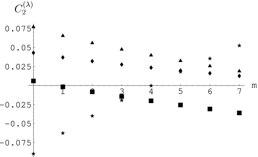
Figure 1: Second-order coefficients $C_{2}^{(\lambda)}(n,m)$ of the exponents $\lambda=\nu_{l2}$ ($\blacklozenge$), $\alpha_{l}$ ($\bigstar$), $\beta_{l}$ ($\blacksquare$), and $\gamma_{l}$ ($\blacktriangle$) for $n=1$ and $m=0,\dots,7$.

4.4 The limit $m\to 0$

In this limit, $d$ ‘perpendicular’ coordinates, but no ‘parallel’ ones remain. Hence ${\boldsymbol{x}}$ can be identified with ${\boldsymbol{x}}_{\perp}$, and the free propagator (7) becomes

$$G({\boldsymbol{x}})=x^{-2+\epsilon}\,\Phi(\upsilon{=}0;m{=}0,d{=}4-\epsilon)=\frac{1}{4}\,\pi^{-d/2}\,x^{-2+\epsilon}\;.$$ (83)

The $\upsilon=0$ value of $\Phi(\upsilon)$ can be read off from the $k=0$ term of the Taylor series (12). The expression on the far right of Eq. (83) is indeed the familiar massless free propagator $[-\triangle]^{-1}({\boldsymbol{x}})$.

We must now determine the $m\to 0$ limits of the integrals $j_{\phi}$, $j_{\sigma}$, $j_{\rho}$, and $J_{u}$ (i.e., $j_{u}$), in terms of which our analytic results given in Secs. 3.2, 3.3, and 4.1 are expressed. We assert that the correct limiting values are

$$j_{\phi}(0)=2\;,\quad j_{\sigma}(0)=j_{\rho}(0)=j_{u}(0)=0\;,\quad J_{u}(0)=\frac{1}{2}\;.$$ (84)

To see this, note that $m$-dimensional integrals $\int\!\d^{m}\upsilon\,f_{m}(\upsilon)=S_{m}\,{\int_{0}^{\infty}}\!\d\upsilon\,f_{m}(\upsilon)\,\upsilon^{m-1}$ should approach their zero-dimensional analog, namely $f_{0}(\upsilon{=}0)$, as $m\to 0$. In the case of $j_{\phi}$, we have $f_{0}(0)=S_{4}\,\Phi^{3}(0;0,4)/F_{0,0}^{2}=2$. The respective values $f_{0}(0)$ for $j_{\sigma}$ and $j_{\rho}$ vanish because of the explicit factors of $\upsilon^{4}$ and $\upsilon^{2}$ appearing in their integrands. On the other hand, the vanishing of $j_{u}(0)$ is due to the factor $\Theta(\upsilon)$ of its integrand and the fact that $\Theta(0)=0$ according to the Taylor series (28). Finally, the value of $J_{u}(0)$ given above follows from $j_{u}(0)=0$ via Eq. (49).

If one sets $m=0$ in the series expansions of quantities whose analogs retain their significance in the case of the usual critical-point theory, e.g., in Eqs. (40), (47), (48), (59), (60), (63), and (67) for $Z_{\phi}$, $Z_{\tau}Z_{\phi}$, $Z_{u}Z_{\phi}^{2}Z_{\sigma}^{m/4}$, $\beta_{u}$, $u^{*}$, $\eta_{\tau}^{*}$, and $\omega_{l2}$, utilizing the above values (84) of the integrals, one recovers the familiar two-loop results for the standard $\phi^{4}$ theory.

Let us also mention that (because of the factor $S_{m}\sim m$ in $B_{m}$) the integrals $j_{\sigma}$, $j_{\rho}$, and $j_{u}$ vanish linearly in $m$ as $m\to 0$. Therefore, quantities like $Z_{\sigma}Z_{\phi}$, $Z_{\rho}Z_{\phi}Z_{\sigma}^{1/2}$, $\eta_{l4}$, $\nu_{l4}$, $\eta_{\rho}^{*}$, $\theta$, etc. that involve ratios such as $j_{\sigma}(m)/m$ have a finite $m\to 0$ limit. It is conceivable that the $m\to 0$ limits of these quantities might turn out to have significance for appropriate problems. However, we shall not further consider this issue here.

4.5 The case of the isotropic Lifshitz point

In the case of an isotropic Lifshitz point one has $d=d_{\|}$ and $d_{\perp}=0$. In a conventional $\epsilon$ expansion one would expand about $d^{*}(8)=8$, setting $d=d_{\|}=8-\epsilon_{\|}$. Results to order $\epsilon_{\|}^{2}$ that have been obtained in this fashion for the correlation exponents $\eta_{l2}$ and $\eta_{l4}$ and the correlation-length exponents $\nu_{l2}$ and $\nu_{l4}$ can be found in Ref. [19].

Since the constraint $d=d_{\|}$ implies that both $d$ and $d_{\|}$ vary as $\epsilon_{\|}$ is varied, it may not be immediately clear that results for this case can be extracted from our $\epsilon$ expansion at fixed $d_{\|}=m$. Let us choose a fixed $m=8-\epsilon_{\|}$ and utilize the $\epsilon$ expansion. This yields

$$\lambda(n,m,d)=\lambda^{(0)}+\lambda^{(1)}(n)\,\epsilon+\lambda^{(2)}(n,m)\,\epsilon^{2}+O(\epsilon^{3})$$ (85)

with $\epsilon=8-d-\epsilon_{\|}/2$, where $\lambda$ means any of the critical exponents considered in Sec. 4.1 that remain meaningful in the case of an isotropic Lifshitz point, such as $\eta_{l4}$, $\nu_{l4}$, $\varphi$, $\alpha_{l}$, $\beta_{q}$, and $\omega_{l4}$. As indicated in Eq. (85), the coefficients of the terms of orders $\epsilon^{0}$ and $\epsilon$ do not depend on $m$. We now set $d=m$, which implies that $\epsilon=\epsilon_{\|}/2$. The upshot is the following: In order to obtain from our $\epsilon$-expansion results the dimensionality expansion of the critical exponents of the isotropic Lifshitz point about $d=8$ to second order, we must simply replace the second-order coefficients $\lambda^{(2)}(n,m)$ by their limiting values $\nu^{(2)}(n,8^{-})$ and identify $\epsilon$ with $\epsilon_{\|}/2=(8-d)/2$.

The limiting values of the integrals $j_{\phi}$, $j_{\sigma}$, $j_{\rho}$, and $J_{u}$ are

$$j_{\phi}(8^{-})=0\;,\quad j_{\sigma}(8^{-})=96\;,\quad j_{\rho}(8^{-})=12\;,\quad J_{u}(8^{-})=-\frac{1}{6}\;.$$ (86)

To see this, note that the factor $B_{m}$ appearing in $j_{\phi}$,…, $j_{u}$ varies $\sim(8{-}m)$ near $m=8$. In the case of $j_{\phi}$, the integral that multiplies $B_{m}$ has a finite $m\to 8$ limit, so $j_{\phi}(8^{-})$ vanishes. By contrast, the corresponding integrals pertaining to $j_{\sigma}$ and $j_{\rho}$ have a pole of first order at $m=8$. We have in $j_{\sigma}$,

$${\int_{0}^{\infty}}\!\d\upsilon\,\upsilon^{m+3}\,\Phi^{3}(\upsilon;m,d^{*}(m)) = {\int_{0}^{\infty}}\!\d w\,w^{7-m}\,f(w)\,[1+O(8-d)]$$ (87)

$$= {f(0)\over 8-m}+O{\left[(8{-}m)^{0}\right]}\;,$$

where $f(w)$ is the function $f(w)\equiv[w^{-4}\,\Phi(1/w;8,8)]^{3}$ whose value $f(0)=(2\,\pi)^{-12}$ follows from Eq. (22). Using this together with ${B^{\prime}}(8)=-3\times 2^{17}\,\pi^{12}$ yields the above result for $j_{\sigma}(8^{-})$. The value of $j_{\rho}(8^{-})$ follows in a completely analogous manner.

The computation of $J_{u}(8^{-})$ is somewhat more involved because the integral giving $j_{u}/B_{m}$ has poles of second and first order. The second-order pole, due to the appearance of the term $\sim\ln\upsilon$ in the large-$\upsilon$ form (30) of the scaling function $\Theta(\upsilon)$, produces a first-order pole in $j_{u}$, which cancels the pole resulting from the contribution $-\frac{1}{2}\,\psi(2{-}{m\over 4})$ to $J_{u}$ [cf. Eq. (49)]. The first-order pole of the integral results in the finite value (86) of $J_{u}(8^{-})$.

Upon substituting the values (86) into the respective $\epsilon$-expansion results of Sec. 4.1 and setting $2\,\epsilon=\epsilon_{\|}=8-d$, we recover indeed the results of Ref. [19] for the correlation exponent $\eta_{l4}$ and the correlation-length exponent $\nu_{l4}$:

$$\eta_{l4}(m{=}d)=-{3\over 20}{n+2\over(n{+}8)^{2}}\,\epsilon_{\|}^{2}+O(\epsilon_{\|}^{3})\;,\quad\epsilon_{\|}\equiv 8-d\;,$$ (88)

and

$$\nu_{l4}(m{=}d)={1\over 4}+{n+2\over 16(n{+}8)}\,\epsilon_{\|}+{(n+2)(15n^{2}+89n+4)\over 960(n{+}8)^{3}}\,\epsilon_{\|}^{2}+O(\epsilon_{\|}^{3})\;.$$ (89)

Furthermore, we can infer the previously unknown series expansions of the remaining exponents of the isotropic Lifshitz point. Specifically for the wave-vector exponent, we find that

$$\beta_{q}(m{=}d)=\frac{2+\eta_{\sigma}^{*}}{4(1+\eta_{\rho}^{*})}=\frac{1}{2}+{21\over 40}\,{n{+}2\over(n{+}8)^{2}}\,\epsilon_{\|}^{2}+O(\epsilon^{3}_{8})\;.$$ (90)

Another significant exponent is the crossover exponent $\varphi$. Its $8-d$ expansion follows from Eq. (90) via the scaling law $\varphi=\nu_{l4}/\beta_{q}$. The one of the correction-to-scaling exponent (68) becomes

$$\omega_{l4}(m{=}d)=\epsilon_{\|}+\frac{202{+}41\,n}{30\,(n{+}8)^{2}}\,\epsilon_{\|}^{2}+O(\epsilon_{\|}^{3})\;.$$ (91)

4.6 Series estimates of the critical exponents for $d=3$ dimensions

We now wish to exploit our $\epsilon$-expansion results of the foregoing subsections to obtain numerical values of the critical exponents in $d=3$ dimensions. We shall mainly consider the cases of uniaxial Lifshitz points ($m=1$) for order-parameter dimensions $n=1,2,3$ and of biaxial ($m=2$) Lifshitz points for $n=1$. Of particular interest is the case $m=n=1$, which is realized by the Lifshitz point of the ANNNI model [7, 38] and is encountered in many experimental systems.

Cases with $m\geq 2$ are of limited interest whenever $n\geq 2$, for the following reason. If a Lifshitz point exists, then low-temperature spin-wave-type excitations whose frequencies vary as $\omega_{\boldsymbol{q}}=\sigma_{0}\,q_{\|}^{4}+q_{\perp}^{2}$ as $\boldsymbol{q}\to 0$ must occur. By analogy with the Mermin-Wagner theorem [39] one concludes that such excitations would destabilize an ordered phase in dimensions $d\leq d_{*}(m)=2+m/2$, ruling out the possibility of a spontaneous breaking of the $O(n)$ symmetry at temperatures $T>0$ for such values of $d$. (This conclusion is in complete accordance with Grest and Sak’s work [40] based on nonlinear sigma models.) Hence in three dimensions one is left with the case $m=1$ of a uniaxial Lifshitz point if $n\geq 2$.

In Table 3 we list numerical estimates of the critical exponents for $d=3$, $n=1$, and $m=1,2,\ldots,6$. For comparison, we also included the $m=0$ values of those critical and correction-to-scaling exponents that go over into their standard counterparts $\nu$, $\gamma$, $\alpha$, $\beta$, and $\omega$ for a critical point. As is explained in the caption, these estimates were either obtained by setting $\epsilon=d^{*}(m)-3$ in the $O(\epsilon^{2})$ expressions of the exponents or else via $[1/1]$ Padé approximants.

Table 3: Numerical estimates for the critical exponents with $n=1$ and $d=3$. The values marked by superscripts $(\epsilon)$ were obtained by setting $\epsilon=1+m/2$ in the expansions to order $\epsilon^{2}$ of the exponents; those marked by superscripts $[1/1]$ were determined from $[1/1]$ Padé approximants whose parameters were fixed by the requirement that the respective expansions to second order in $\epsilon$ are reproduced.

$m$	0	1	2	3	4	5	6
$\nu_{l2}^{(\epsilon)}$	0.627	0.709	0.795	0.882	0.963	1.035	1.093
$\nu_{l2}^{[1/1]}$	0.673	0.877	1.230	1.742	2.190	2.260	2.020
$\nu_{l4}^{(\epsilon)}$	—	0.348	0.387	0.423	0.456	0.482	0.500
$\nu_{l4}^{[1/1]}$	—	0.396	0.482	0.561	0.606	0.609	0.585
$\gamma_{l}^{(\epsilon)}$	1.244	1.397	1.558	1.715	1.859	1.983	2.080
$\gamma_{l}^{[1/1]}$	1.310	1.609	2.020	2.460	2.780	2.860	2.750
$\alpha_{l}^{(\epsilon)}$	0.077	0.110	0.174	0.296	0.499	0.806	1.240
$\alpha_{l}^{[1/1]}$	0.108	0.160	0.226	0.323	0.499	0.94	4.600
$\beta_{l}^{(\epsilon)}$	0.340	0.247	0.134	-0.005	-0.180	-0.390	-0.700
$\beta_{l}^{[1/1]}$	0.339	0.246	0.131	-0.029	-0.280	-0.750	-2.000
$\varphi^{(\epsilon)}$	—	0.677	0.686	0.636	0.514	0.306	0.001
$\varphi^{[1/1]}$	—	0.715	0.688	0.654	0.628	0.609	0.595
$\omega_{l2}^{(\epsilon)}$	0.370	0.414	0.553	0.240	-0.255	-0.930	-1.786
$\omega_{l2}^{[1/1]}$	0.614	0.870	1.161	1.313	1.439	1.545	1.635

According to Table 2, the coefficients of most of these series with $n=1$ do not alternate in sign. Exceptions are the ones of $\alpha_{l}$ and $\omega_{l2}$ for small values of $m$, that of $\beta_{l}$ for $m=0$ (i.e., of the usual critical index $\beta$), and the one of $\varphi$ for larger values of $m$. For $d=3$, the second-order contributions grow very rapidly as $m$ increases because of the factor $\epsilon^{2}=(1+m/2)^{2}$. Therefore the numerical estimates become less reliable for large $m$. This effect is more pronounced for $[1/1]$ estimates from non-alternating series than for the corresponding direct evaluations at $d=3$ (marked by superscripts ${(\epsilon)}$). The better-behaved expansions yield smaller differences between these two kinds of estimates. In unfavorable cases with rather large $\epsilon$ we reject the $[1/1]$ estimates for the non-alternating series, which tend to overestimate the values of the corresponding exponents. Instead we prefer the direct evaluations at $d=3$.

A reversed situation occurs for $\alpha_{l}$ and $\omega_{l2}$ with $m=0,1,2$. The respective series are alternating; they have negative $O(\epsilon^{2})$ corrections, which tend to underestimate the values of the exponents for $d=3$ in direct evaluations of the $O(\epsilon^{2})$ expressions. On the other hand, the $[1/1]$ approximants for these series seem to do a better job, suppressing the influence of the second-order corrections in a correct way. We believe that $\alpha_{l}^{[1/1]}(m{=}n{=}1)\simeq 0.160$ belongs to our best numerical $d=3$ estimates that are obtainable from the individual $\epsilon$ expansions.

In the case of $\omega_{l2}$, the second-order correction is much larger. While therefore less accurate numerical estimates must be expected, the structure of the $\epsilon$ expansion for $\omega_{l2}$ suggests nevertheless that this correction-to-scaling exponent should have a larger value than its $m=0$ counterpart $\omega$ for the critical point. (Recall that the latter has a value close to $0.8$ [41]). Our best estimate is the $[1/1]$ value

$$\omega_{l2}\simeq 0.870\;.$$ (92)

In order to obtain improved estimates we proceed as follows. We choose the “best” $d=3$ estimates we can get from the apparently best-behaved $\epsilon$ expansions of certain exponents, express the remaining critical indices in terms of the former, and compute their implied values. Thus we select from Table 3 the numbers

$$\nu_{l4}^{(\epsilon)}(d{=}3;m{=}1,n{=}1)\simeq 0.348\quad\mbox{and}\quad\alpha_{l}^{[1/1]}(3;1,1)\simeq 0.160\;,$$ (93)

which we complement by our estimate

$$\eta_{l4}(3;,1,1)\simeq-0.019$$ (94)

from I. Substituting these into the second one of the scaling relations (80) for $\gamma_{l}$ and the hyperscaling relation (78) for $\alpha_{l}$ yields

$$\gamma_{l}(3;1,1)\simeq 1.399\quad\mbox{and}\quad\nu_{l2}(3;1,1)\simeq 0.746\;,$$ (95)

respectively, from which in turn the values

$$\eta_{l2}(3;1,1)\simeq 0.124\quad\mbox{and}\quad\beta_{l}(3;1,1)\simeq 0.220$$ (96)

follow via the scaling relations $\eta_{l2}=2-\gamma_{l}/\nu_{l2}$ and $\beta_{l}=(2-\alpha_{l}-\gamma_{l})/2$.

Likewise, the choices

$$\varphi(3;1,1)\simeq\varphi^{(\epsilon)}=0.677\quad\mbox{and}\quad\nu_{l4}(3;1,1)\simeq\nu_{l4}^{(\epsilon)}=0.348$$ (97)

give for the wave-vector exponent

$$\beta_{q}={\nu_{l4}/\varphi}$$ (98)

the estimate

$$\beta_{q}(3;1,1)\simeq 0.514\;,$$ (99)

which is fairly close to the value $\beta_{q}\simeq 0.519$ of I. We consider the values (92)–(97) and (99) as our best estimates for these 10 critical exponents.

Table 4: Critical exponents for $m=1$, $n=1$, $2$, $3$, and $d=3$. The row marked MF gives the mean-field values; rows marked $O(\epsilon)$ and $O(\epsilon^{2})$ list the values obtained by setting $\epsilon=3/2$ in the expansions to first and second order in $\epsilon$, respectively. The remaining rows contain the estimates from $[1/1]$ Padé approximants and our “best” estimates (‘Scal.’) obtained via scaling relations in the manner explained in the main text.

		$n=1$				$n=2$		$n=3$
	MF	$O(\epsilon)$	$O(\epsilon^{2})$	$[1/1]$	Scal.	$O(\epsilon)$	$O(\epsilon^{2})$	$O(\epsilon)$	$O(\epsilon^{2})$
$\nu_{l2}$	${1\over 2}$	0.625	0.709	0.877	0.746	0.650	0.757	0.670	0.798
$\nu_{l4}$	${1\over 4}$	0.313	0.348	0.396	0.348	0.325	0.372	0.335	0.392
$\alpha_{l}$	0	0.250	0.110	0.160	0.160	0.150	-0.047	0.068	-0.178
$\beta_{l}$	${1\over 2}$	0.250	0.247	0.246	0.220	0.275	0.276	0.295	0.301
$\gamma_{l}$	1	1.250	1.397	1.609	1.399	1.300	1.495	1.340	1.576
$\varphi$	${1\over 2}$	0.625	0.677	0.715	0.677	0.650	0.725	0.670	0.765
$\beta_{q}$	${1\over 2}$	0.500	0.519		0.514	0.500	0.521	0.500	0.521
$\eta_{l2}$	0	0	0.039		0.124	0	0.042	0	0.044
$\eta_{l4}$	0	0	-0.019		-0.019	0	-0.020	0	-0.021
$\omega_{l2}$	0	1.500	0.414	0.870		1.500	0.466	1.500	0.517

Table 4 presents an overview of our numerical findings. For convenience, the mean-field results are included along with the values the $\epsilon$ expansions to first and second order take at $\epsilon=3/2$. The case $m=1$ with $n=2$ corresponds to the Lifshitz point of the axial next-nearest-neighbor XY (ANNNXY) model, which Selke studied many years ago by means of Monte Carlo simulations [42].

In Table 5 we have gathered the available experimental results for critical exponents together with estimates obtained from Monte Carlo calculations and high-temperature series analyses. As one sees, our field-theory estimates are in a good agreement with the Monte Carlo results. The experimental value for $\alpha_{l}(3;1,1)$ deviates appreciably both from all theoretical estimates (including ours) as well as from the Monte Carlo results, and is probably not very accurate. On the other hand, the very good agreement of our field-theory estimates with the most recent Monte Carlo estimates by Pleimling and Henkel [27] (which we expect to be the most accurate ones) is quite encouraging. Certainly, renewed experimental efforts for determining the values of the critical exponents in a more complete and more precise way would be most welcome.

Table 5: Values of critical exponents for uniaxial Lifshitz points ($m{=}1$). ‘Exp’ means summarized experimental results, taken from Ref. [43]; ‘HT’ denotes the high-temperature series estimates of Ref. [44]. The rest are the Monte Carlo results of Refs. [45] (MC1), [46] (MC2), [27] (MC3), and [42] (MC), respectively.

	$\nu_{l4}$	$\alpha_{l}$	$\beta_{l}$	$\gamma_{l}$	$\varphi$	$\beta_{q}$
	$n=1$
Exp		0.4–0.5			0.60–0.64	0.44–0.49
HT	$0.41{\pm}0.03$	0.20${\pm}$0.15		1.62${\pm}$0.12		0.5
MC1			0.21${\pm}$0.03	1.36${\pm}$0.005
MC2	0.33${\pm}$0.03	0.2	0.19${\pm}$0.02	1.4${\pm}$0.06
MC3		0.18${\pm}$0.03	0.235${\pm}$0.005	1.36${\pm}$0.03
	$n=2$
MC		0.1${\pm}$0.14	0.20${\pm}$0.02	1.5${\pm}$0.1

5 Concluding remarks

The field-theory models (3) were introduced more than 25 years ago to describe the universal critical behavior at $m$-axial Lifshitz points [19]. While some field-theoretic studies based on the $\epsilon$ expansion about the upper critical dimension $d^{*}(m)$ emerged soon afterwards, these were limited to first order in $\epsilon$, or restricted to special values of $m$ or to a subset of critical exponents, or challenged by discrepant results (see the references cited in the introduction). Two-loop calculations for general values of $m$ appeared to be hardly feasible because of the severe calculational difficulties that must be overcome.

Complementing our previous work in I, we have presented here a full two-loop RG calculation for the models (3) in $d=d^{*}(m)-\epsilon$ dimensions, for general values of $m\in(0,8)$. This enabled us to compute the $\epsilon$ expansions of all critical indices of the considered $m$-axial Lifshitz points to second order in $\epsilon$. We employed these results in turn to determine field-theory estimates for the values of these critical exponents in three dimensions. Although the accuracy of these estimates clearly is not competitive with the impressive precision that has been achieved by the best field-theory estimates for critical exponents of conventional critical points (based on perturbation expansions to much higher orders and powerful resummation techniques [41, 4]), they are in very good agreement with recent Monte Carlo results for the uniaxial scalar case $m=n=1$. We hope that our present work will stimulate new efforts, both by experimentalists and theorists, to investigate the critical behavior at Lifshitz points.

There is a number of promising directions in which our work could be extended. For example, building on it, one could compute other universal quantities, such as amplitude ratios and scaling functions, via the $\epsilon$ expansion.

A particular interesting and challenging question is whether the generalized invariance found by Henkel [25] for systems whose anisotropy exponents take the rational values $\theta=2/\wp$, $\wp=1,2,3\ldots$ can be generalized to other, irrational values. That such an extension exists, is not at all clear since the condition $\theta=2/\wp$ is utilized in Henkel’s work to ensure that the algebra closes. But if such an extension can be found, then the invariance under this larger group of transformations should manifest itself through properties of the theories’ scaling functions in $d<d^{*}(m)$ dimensions, which could be checked by means of the $\epsilon$ expansion. Furthermore, even if an extension cannot be found, one should be able to benefit from the invariance properties of the free theory (with $\theta=1/2$) when computing the $\epsilon$ expansion of anomalous dimensions of composite operators in a similar extensive fashion as in the case of the standard critical-point $\phi^{4}$ theory [47, 48, 49].

An important issue awaiting clarification arises when $m\geq 2$. In the class of models (3) studied here, the quadratic fourth-order derivative term was taken to be isotropic in the subspace ${\mathbb{R}}^{m}$. However, in general further fourth-order derivatives cannot be excluded. That is, the term $(\sigma_{0}/2)\,(\triangle_{\|}\boldsymbol{\phi})^{2}$ should be generalized to

$$(\sigma_{0}/2)\,w_{a}\,T^{(a)}_{ijkl}\,(\partial_{i}\partial_{j}{\boldsymbol{\phi}})\partial_{k}\partial_{l}\,{\boldsymbol{\phi}}\;,$$ (100)

where the summation over $a$ comprises all totally symmetric fourth-rank tensors $T^{(a)}_{ijkl}$ compatible with the symmetry of the considered microscopic (or mesoscopic) model. The isotropic fourth-order derivative term corresponds to $T^{(a{=}1)}_{ijkl}\equiv(\delta_{ij}\,\delta_{kl}+\delta_{ik}\,\delta_{jl}+\delta_{il}\,\delta_{jk})/3$ with $w_{1}\equiv 1$.

In order to give a simple example of a system involving a further quadratic fourth-order derivative term, let us consider an $m$-axial modification of the familiar uniaxial ANNNI model [38, 7] that has competing nearest-neighbor (nn) and next-nearest-neighbor interactions along $m$ equivalent of the $d$ hypercubic axes (and only the usual nn bonds along the remaining $d-m$ ones). Owing to the Hamiltonian’s hypercubic (rather than isotropic) symmetry in the $m$-dimensional subspace, just one other fourth-order derivative term, corresponding to the tensor $T^{(2)}_{ijkl}=\delta_{ij}\delta_{kl}\delta_{li}$, must generically occur besides the isotropic one, in a coarse-grained description. The associated interaction constant $w_{2}$ is dimensionless and hence marginal at the Gaussian fixed point. To find out whether the nontrivial ($u^{*}>0$, $w_{2}=0$) fixed point considered throughout this work remains infrared stable, one must compute the anomalous dimension of the additional scaling operator that can be formed from the above two fourth-order derivative terms. This issue will be taken up in a forthcoming joint paper with R. K. P. Zia [50], where we shall show that the associated crossover exponent, to order $\epsilon^{2}$, is indeed positive. Hence, deviations from $w_{2}=0$ correspond to a relevant perturbation at the $w_{2}=0$, $u^{*}>0$ fixed point, which should destabilize it unless $m=1$.

Finally, let us mention that the potential of the $\epsilon$-expansion results presented in this paper certainly has not fully been exploited here. When estimating the values of the critical exponents for $d=3$ dimensions, we utilized only their $\epsilon$ expansions for a fixed integer number of the parameter $m$. However, our results hold also for noninteger values of $m$. Making use of this fact, one should be able to extrapolate to points $(d=3,m=\mbox{integer})$ of interest in a more flexible fashion, starting from any point on the critical curve $d=d^{*}(m)$ and going along directions not perpendicular to the $m$ axis. By exploiting this flexibility one should be able to improve the accuracy of the estimates.

Last but not least, let us briefly mention where the interesting reader can find information about experimental results. Earlier experimental work is discussed in Hornreich’s and Selke’s review articles [6, 7]. A more recent summary of experimental results for the critical exponents and other universal quantities of the Lifshitz point in MnP and Mn_0.9Co_0.1P can be found in Ref. [43] and its references. (These results were partly quoted in Table 5.) However, the variety of experimental systems having (or believed to have) Lifshitz points is very rich, ranging from ferromagnetic and ferroelectric systems to polymer mixtures. A complete survey of the published experimental results on Lifshitz points is beyond the scope of the present article.

Appendix A Series representation and asymptotic expansion of $\Phi(\upsilon)$

¿From the integral representation (8) of the scaling function $\Phi(\upsilon)$ we find

$$\Phi(\upsilon) = \int_{{\boldsymbol{q}}_{\|}}\int_{{\boldsymbol{q}}_{\perp}}{\e^{i{\boldsymbol{q}}_{\perp}\cdot{\boldsymbol{e}}_{\perp}}\,\e^{i{\boldsymbol{q}}_{\|}\cdot\boldsymbol{\upsilon}}\over q_{\perp}^{2}+q_{\|}^{4}}={\upsilon}^{-4+2\epsilon}\int_{{\boldsymbol{q}}_{\|}}\int_{{\boldsymbol{q}}_{\perp}}{\e^{i\upsilon^{-2}{\boldsymbol{q}}_{\perp}\cdot{\boldsymbol{e}}_{\perp}}\,\e^{i{\boldsymbol{q}}_{\|}\cdot{\boldsymbol{e}}_{\|}}\over q_{\perp}^{2}+q_{\|}^{4}}\;,$$ (101)

where ${\boldsymbol{e}}_{\|}=\boldsymbol{\upsilon}/\upsilon$ is an arbitrary unit $m$-vector. The second form follows via rescaling of the momenta; it lends itself for studying the large-$\upsilon$ behavior. The first one is appropriate for deriving the small-$\upsilon$ expansion.

Upon utilizing the Schwinger representation

$$\frac{1}{q_{\perp}^{2}+q_{\|}^{4}}={\int_{0}^{\infty}}\!{\d}s\,\e^{-s\,\big{(}q_{\perp}^{2}+q_{\|}^{4}\big{)}}$$ (102)

for the momentum-space propagator in Eq. (101), we can perform the integration over ${\boldsymbol{q}}_{\perp}$ to obtain

$$\Phi(\upsilon) = (4\,\pi)^{-d_{\perp}/2}\,{\upsilon}^{-4+2\epsilon}{\int_{0}^{\infty}}\!\d s\,s^{-d_{\perp}/2}\int_{{\boldsymbol{q}}_{\|}}\e^{-s\,q_{\|}^{4}-({4\,s\,\upsilon^{4})}^{-1}}\e^{i{\boldsymbol{q}}_{\|}\cdot{\boldsymbol{e}}_{\|}}\;.$$ (103)

Doing the angular integrations gives

$$\int_{{\boldsymbol{q}}_{\|}}\e^{-s\,q_{\|}^{4}}\e^{i{\boldsymbol{q}}_{\|}\cdot{\boldsymbol{e}}_{\|}}=(2\,\pi)^{-m/2}\,{\int_{0}^{\infty}}\!\d q\,q^{m/2}\,J_{m-2\over 2}(q)\,\e^{-s\,q^{4}}\;.$$ (104)

We insert this into Eq. (103), expand the exponential $\e^{-1/(4\,s\,\upsilon^{4})}$ in powers of $\upsilon^{-4}$, and integrate the resulting series termwise over $s$. This yields

$$\Phi(\upsilon) = 2^{-2-m}\,\pi^{-{d-1\over 2}}\,{\left({\upsilon\over 2}\right)}^{2\,\epsilon-4}\sum_{k=0}^{\infty}\frac{(-1)^{k}}{k!}\,\Phi_{k}\,{\left({\upsilon\over 2}\right)}^{-4k}$$ (105)

with

$$\Phi_{k} = {\Gamma{\left(\frac{m}{4}-1-k-\frac{\epsilon}{2}\right)}\over 2^{6-m+6k-3\,\epsilon}}\;{\int_{0}^{\infty}}\!\d q\,{q^{4(1+k)-{\frac{m}{2}}-2\,\epsilon}}\,J_{m-2\over 2}(q)$$ (106)

$$= {\frac{2\,\Gamma(2+2k-\epsilon)}{\Gamma{\left(\frac{m}{4}-\frac{1}{2}+\frac{\epsilon}{2}-k\right)}}}\;,$$

which is the asymptotic expansion (15). The Taylor series (12) can be derived along similar lines, starting from the first form of the integral representation (101).

Appendix B Laurent expansion of required vertex functions

In this appendix we gather our results on the Laurent expansions of those vertex functions whose pole terms determine the required renormalization factors. It is understood that $\tau_{0}$ and $\rho_{0}$ are set to their critical values $\tau_{c}=\rho_{c}=0$. For notational simplicity, we introduce the dimensionless bare coupling constant

$$\check{u}_{0}\equiv\mu^{-\epsilon}\,\sigma_{0}^{-m/4}\,u_{0}=Z_{u}\,u$$ (107)

and specialize to the scalar case $n=1$. The generalization to the $n$-component case involves the usual tensorial factors and contractions of the standard $|\boldsymbol{\phi}|^{4}$ theory and should be obvious.

We use the notation $\tilde{\Gamma}(\{{\boldsymbol{q}}_{j}\})$ for the Fourier transforms of vertex functions $\Gamma(\{\boldsymbol{x}_{j}\})$ (with the momentum-conserving $\delta$ function taken out):

$$\Gamma(\{\boldsymbol{x}_{j}\})=\int_{{\boldsymbol{q}}_{1},\ldots,{\boldsymbol{q}}_{N}}\tilde{\Gamma}(\{{\boldsymbol{q}}_{j}\})\,(2\,\pi)^{d}\,\delta{\bigg{(}\sum_{j}\boldsymbol{q}_{j}\bigg{)}}\,\e^{i\sum_{j=1}^{N}\boldsymbol{q}_{j}\cdot\boldsymbol{x}_{j}}\;.$$ (108)

B.1 Two-point vertex functions $\Gamma^{(2)}$ and $\Gamma^{(2)}_{(\nabla_{\|}\phi)^{2}}$

¿From our results obtained in I we find

$$\tilde{\Gamma}^{(2)}({\boldsymbol{q}})=\sigma_{0}q_{\|}^{4}+q_{\perp}^{2}-\raisebox{-4.25pt}{ \texdraw \drawdim pt \setunitscale 2.5 \linewd 0.3 \lellip rx:5 ry:2.8 \move(-8 0) \lvec(8 0) }\;+O(u_{0}^{3})$$ (109)

with

$$\raisebox{-4.25pt}{ \texdraw \drawdim pt \setunitscale 2.5 \linewd 0.3 \lellip rx:5 ry:2.8 \move(-8 0) \lvec(8 0) }\;={\check{u}_{0}^{2}\over 6\,\epsilon}\,{\left[{j_{\sigma}(m)\,\sigma_{0}\,q_{\|}^{4}\over 16\,m(m{+}2)}-\frac{{j}_{\phi}(m)\,q_{\perp}^{2}}{2\,(8-m)}\right]}+O(\epsilon^{0})$$ (110)

and

$$\tilde{\Gamma}^{(2)}_{(\nabla_{\|}\phi)^{2}}({\boldsymbol{q}},{\boldsymbol{Q}}={\boldsymbol{0}})=q_{\|}^{2}-\raisebox{-4.25pt}{ \texdraw \drawdim pt \setunitscale 2.5 \linewd 0.3 \lellip rx:5 ry:2.8 \move(-8 0) \lvec(8 0) \move(0 2.8) \fcir f:0 r:0.7 \rmove(-1.15 -1)\rlvec(0 2) \rmove(2.25 -2)\rlvec(0 2) }\;+O(u_{0}^{3})$$ (111)

with

$$\raisebox{-4.25pt}{ \texdraw \drawdim pt \setunitscale 2.5 \linewd 0.3 \lellip rx:5 ry:2.8 \move(-8 0) \lvec(8 0) \move(0 2.8) \fcir f:0 r:0.7 \rmove(-1.15 -1)\rlvec(0 2) \rmove(2.25 -2)\rlvec(0 2) }={\check{u}_{0}^{2}\over 2\,\epsilon}\,{j_{\rho}(m)\over 4\,m}\,q_{\|}^{2}+O(\epsilon^{0})\;,$$ (112)

where $\boldsymbol{Q}=\boldsymbol{0}$ is the momentum of the inserted operator $(\nabla_{\|}\phi)^{2}/2$; i.e., the insertion considered is ${\int}\d^{d}x(\nabla_{\|}\phi)^{2}/2$.

B.2 Four-point vertex function $\Gamma^{(4)}$

The four-point vertex function was computed only to one-loop order in I. To the order of two loops it reads

$$\tilde{\Gamma}^{(4)}({\boldsymbol{q}}_{1},\ldots,{\boldsymbol{q}}_{4}) = u_{0}-\left(\;\raisebox{-2.2pt}{\texdraw \drawdim pt \setunitscale 2.5 \linewd 0.3 \lellip rx:4 ry:1.8 \move(4 0)\rlvec(2 2) \move(4 0)\rlvec(2 -2) \move(-4 0)\rlvec(-2 -2) \move(-4 0)\rlvec(-2 2) }+2\,\mathcal{P\/}\right)-\left(\;\raisebox{-2.2pt}{\texdraw \drawdim pt \setunitscale 2.5 \linewd 0.3 \lellip rx:4 ry:1.8 \move(-4 0)\rlvec(-2 -2) \move(-4 0)\rlvec(-2 2) \move(8 0) \lellip rx:4 ry:1.8 \move(12 0)\rlvec(2 2) \move(12 0)\rlvec(2 -2) }+2\,\mathcal{P\/}\right)$$ (114)

$$\mbox{}-\left(\;\raisebox{-8.0pt}{\texdraw \drawdim pt \setunitscale 2.5 \linewd 0.3 \move(-7 -1.5)\rlvec(15 6) \move(-7 1.5)\rlvec(15 -6) \move(5 0) \lellip rx:1 ry:3 }+5\,\mathcal{P}\right)+O(u_{0}^{4})$$

$$= u_{0}{\left\{1-\sum_{(ij)=(12),(23),(24)}{\left[{\check{u}_{0}\over 2}\,I_{2}(\check{\boldsymbol{q}}_{ij})-{\check{u}^{2}_{0}\over 4}\,I_{2}^{2}(\check{\boldsymbol{q}}_{ij})\right]}\right.}$$

$${\left.\mbox{}+\frac{\check{u}_{0}^{2}}{2}\,{\left[I_{4}(\check{\boldsymbol{q}}_{12},\check{\boldsymbol{q}}_{3})+5\,\mathcal{P}\right]}\right\}}\;.$$

Here $\mathcal{P}$ means permutations (of the external legs). The hatted momenta are dimensionless ones defined via

$$\check{\boldsymbol{q}}=(\check{\boldsymbol{q}}_{\|},\check{\boldsymbol{q}}_{\perp})\equiv{\left(\sigma_{0}^{1/4}\,\mu^{-1/2}\,{\boldsymbol{q}}_{\|},\mu^{-1}\,{\boldsymbol{q}}_{\perp}\right)}\;,$$ (115)

and $\check{\boldsymbol{q}}_{ij}\equiv\check{\boldsymbol{q}}_{i}+\check{\boldsymbol{q}}_{j}$. The integrals $I_{2}$ and $I_{4}$ are given by

$$I_{2}({\boldsymbol{Q}})\equiv\int_{\boldsymbol{q}}\,{1\over q_{\perp}^{2}+q_{\|}^{4}}\,{1\over{\Big{(}{\boldsymbol{q}}+{\boldsymbol{Q}}\Big{)}}_{\perp}^{2}+{\left({\boldsymbol{q}}+{\boldsymbol{Q}}\right)}_{\|}^{4}}$$ (116)

and

$$I_{4}({\boldsymbol{Q}},{\boldsymbol{K}})\equiv\int_{{\boldsymbol{q}}}\,{1\over q_{\perp}^{2}+q_{\|}^{4}}\,{1\over{\left({\boldsymbol{q}}+{\boldsymbol{Q}}\right)}_{\perp}^{2}+{\left({\boldsymbol{q}}+{\boldsymbol{Q}}\right)}_{\|}^{4}}\,I_{2}({\boldsymbol{q}}-{\boldsymbol{K}})\;.$$ (117)

The pole term of $I_{2}({\boldsymbol{Q}})$ can be read off from Eqs. (24) and (89) of I. However, in our two-loop calculation $I_{2}$ also occurs as a divergent subintegral. To check that the associated pole terms are canceled by contributions involving one-loop counterterms, we also need the finite part of $I_{2}$. The calculation simplifies considerably if the momentum $\boldsymbol{Q}$ is chosen to have a perpendicular component only, so that $\boldsymbol{Q}=Q\,{\boldsymbol{e}}_{\perp}$ (which is sufficient for our purposes). For such values of ${\boldsymbol{Q}}$, the integral $I_{2}({\boldsymbol{Q}})$ can be analytically calculated in a straightforward fashion, either by going back to Eq. (16) and (19) of I and computing the Fourier transform of these distributions, or directly in momentum space, as we prefer to do here. For dimensional reasons, we have

$$I_{2}(Q\,{\boldsymbol{e}}_{\perp})=Q^{-\epsilon}\,I_{2}({\boldsymbol{e}}_{\perp})\;.$$ (118)

The integral on the right-hand side is precisely the one written as $F_{m,\epsilon}/\epsilon$ in Eq. (38). Utilizing a familiar method due to Feynman for folding two denominators into one (Eq. (A8-1) of Ref. [36]), one is led to

$$I_{2}({\boldsymbol{e}}_{\perp}) = {\int_{0}^{1}}\!\d{s}\int_{\boldsymbol{q}}\left[q_{\|}^{4}+q_{\perp}^{2}+2\,s\,{{\boldsymbol{q}}_{\perp}}\cdot{\boldsymbol{e}}_{\perp}+s\,{\boldsymbol{e}}_{\perp}^{2}\right]^{-2}$$ (119)

$$= 2^{-4+\frac{m}{2}+\epsilon}\,\pi^{-2+\frac{m}{4}+\frac{\epsilon}{2}}\,\Gamma{\left(\frac{m+2\,\epsilon}{4}\right)}{\int_{0}^{1}\!}\d s\int_{{\boldsymbol{q}}_{\|}}{\left[q_{\|}^{4}+s(1-s)\right]}^{-{m+2\,\epsilon\over 4}}$$

$$= (4\,\pi)^{-d/2}\,{\Gamma{\left(\frac{m}{4}\right)}\,\Gamma{\left(\frac{\epsilon}{2}\right)}\,\Gamma^{2}{\left(1-\frac{\epsilon}{2}\right)}\over 2\,\Gamma(2-\epsilon)\,\Gamma{\left(\frac{m}{2}\right)}}\;,$$

from which the result (39) for $F_{m,\epsilon}$ follows at once.

The calculation of $I_{4}({\boldsymbol{Q}},{\boldsymbol{K}})$ is more involved; it is described in Appendix C, giving

$$I_{4}(Q\,{\boldsymbol{e}}_{\perp},{\boldsymbol{K}})=F_{m,\epsilon}^{2}\,{Q^{-2\epsilon}\over 2\epsilon}\,{\left[\frac{1}{\epsilon}+J_{u}(m)+O(\epsilon)\right]}\;,$$ (120)

where $J_{u}(m)$ is the quantity defined in Eq. (49).

B.3 Vertex function $\Gamma^{(2)}_{\phi^{2}}$

Next, we turn to the vertex function $\Gamma^{(2)}_{\phi^{2}}$ with an insertion of $\frac{1}{2}(\phi^{2})_{{\boldsymbol{Q}}}=\frac{1}{2}{\int}\d^{d}x\,\phi^{2}({\boldsymbol{x}})\,\e^{i\,{\boldsymbol{Q}}\cdot{\boldsymbol{x}}}$. To two-loop order it is given by

$$\Gamma^{(2)}_{\phi^{2}}({\boldsymbol{q}};\boldsymbol{Q}) = 1-\;\raisebox{-3.0pt}{\texdraw\drawdim pt \setunitscale 2.5 \linewd 0.3 \lellip rx:2.8 ry:2.8 \move(0 2.8)\fcir f:0 r:0.5 \move(-3 -2.8) \rlvec(6 0) }\;-\;\raisebox{-3.0pt}{\texdraw\drawdim pt \setunitscale 2.5 \linewd 0.3 \lcir r:2.0 \move(0 4) \lcir r:2.0 \move(0 6)\fcir f:0 r:0.5 \move(-3 -2) \rlvec(6 0) }\;-\raisebox{-4.25pt}{ \texdraw \drawdim pt \setunitscale 2.5 \linewd 0.3 \lellip rx:5 ry:2.8 \move(-8 0) \lvec(8 0) \move(0 2.8) \fcir f:0 r:0.7 }\;+O(u_{0}^{3})$$ (121)

$$= 1-{\check{u}_{0}\over 2}\,I_{2}(\check{\boldsymbol{Q}})+{\check{u}^{2}_{0}}\,{\left[\frac{1}{4}\,I_{2}^{2}(\check{\boldsymbol{Q}})+\frac{1}{2}\,I_{4}(\check{\boldsymbol{Q}},\check{\boldsymbol{q}})\right]}+O(u_{0}^{3})\;,$$

where the hatted momenta are again dimensionless ones, defined by analogy with Eq. (115).

Appendix C Laurent expansion of the two-loop integral ${\boldsymbol{I_{4}}}$

As can be seen from Eq. (117), the integral $I_{4}(\check{\boldsymbol{q}}_{12},\check{\boldsymbol{q}}_{3})$ associated with the graph pt 1.5 0.3 (-7 -1.5)(15 6) (-7 1.5)(15 -6) (5 0) rx:1 ry:3 involves the divergent subintegral $I_{2}(\check{\boldsymbol{q}}-\check{\boldsymbol{q}}_{3})$. The latter has a momentum-independent pole term $\sim\epsilon^{-1}$ [cf. Eqs. (119) and (39)]. Furthermore, the graph that results upon contraction of this subgraph to a point [which itself is proportional to $I_{2}(\check{\boldsymbol{q}}_{12}$)] has contributions of order $\epsilon^{0}$ that depend on $\check{q}_{12}$. Taken together, these observations tell us that the pole term $\propto\epsilon^{-1}$ of $I_{4}(\check{\boldsymbol{q}}_{12},\check{\boldsymbol{q}}_{3})$ depends on $\check{q}_{12}$ but not on $\check{q}_{3}$. Since the $\epsilon^{-2}$ pole of $I_{4}(\check{\boldsymbol{q}}_{12},\check{\boldsymbol{q}}_{3})$ is momentum independent, we can set $\check{q}_{3}=0$ when calculating the pole part of this integral.

To further simplify the calculation, we can choose $\check{\boldsymbol{q}}_{12}$ to have vanishing parallel component again, setting $\check{\boldsymbol{q}}_{12}=Q\,{\boldsymbol{e}}_{\perp}$. The integral to be calculated thus becomes

$$I_{4}(Q\,{\boldsymbol{e}}_{\perp};{\boldsymbol{0}})={\int}\!\d^{d}{x}{\int}\!\d^{d}{y}\,G({\boldsymbol{y}})\,G({\boldsymbol{x}}-{\boldsymbol{y}})\,\e^{i\,Q\,\boldsymbol{e}_{\perp}\cdot\boldsymbol{y}}\,G^{2}({\boldsymbol{x}})\,,$$ (122)

where $G({\boldsymbol{y}})$ now means the free propagator (5) with $\sigma_{0}=1$. Let us substitute the free propagators of the factor $G^{2}({\boldsymbol{x}})$ by their scaling form (7) and rewrite the Fourier integral ${\int}\!\d^{d}{y}\dots$ as a momentum-space integral, employing the Schwinger representation (102) for both of the two free propagators in momentum space. Making the change of variables ${\boldsymbol{x}}_{\|}\to{\boldsymbol{\upsilon}}={{\boldsymbol{x}}_{\|}}\,x_{\perp}^{-1/2}$, we arrive at

$$I_{4}(Q\,{\boldsymbol{e}}_{\perp},{\boldsymbol{0}}) = {\int}\!\d^{m}\upsilon\,\Phi^{2}(\upsilon){\int}\!\d^{d-m}{x_{\perp}}\,x_{\perp}^{2\,\epsilon+{m\over 2}-4}\,{\int_{0}^{\infty}}\!\d{s}{\int_{0}^{\infty}}\!\d{t}$$ (123)

$$\times \int_{{\boldsymbol{q}}_{\perp}}\e^{-q_{\perp}^{2}\,(s+t)+{{\boldsymbol{q}}_{\perp}}\cdot{(i\,\boldsymbol{x}_{\perp}-2\,t\,Q\,{\boldsymbol{e}}_{\perp})}-t\,Q^{2}}\,\int_{{\boldsymbol{q}}_{\|}}\e^{-q_{\|}^{4}\,(s+t)+i\,{\boldsymbol{q}}_{\|}\cdot{\boldsymbol{\upsilon}}\sqrt{x_{\perp}}}.$$

Now the momentum integrations $\int_{{\boldsymbol{q}}_{\perp}}$ and $\int_{{\boldsymbol{q}}_{\|}}$ are decoupled and can be performed in a straightforward fashion. That the latter integral takes such a simple form is due to our choice of $\boldsymbol{Q}$ with ${\boldsymbol{Q}}_{\|}=\boldsymbol{0}$. Performing the angular integrations yields

$$\int_{{\boldsymbol{q}}_{\|}}\e^{-q_{\|}^{4}\,(s+t)+i\,{\boldsymbol{q}}_{\|}\cdot{\boldsymbol{\upsilon}}\sqrt{x_{\perp}}}$$ (124)

$$=(2\pi)^{-{m\over 2}}\int_{0}^{\infty}\!\d q_{\|}\,q_{\|}^{m\over 2}\,\e^{-q_{\|}^{4}\,(s+t)}\,(\upsilon^{2}\,x_{\perp})^{{2-m\over 4}}J_{m-2\over 2}{\left(q_{\|}\,\upsilon\,x_{\perp}^{1/2}\right)}\;.$$

We replace the Bessel function in Eq. (124) by its familiar Taylor expansion

$$J_{\mu}(w)={\left({w\over 2}\right)}^{\mu}\,\sum_{k=0}^{\infty}{(-1)^{k}\,w^{2k}\over 2^{2k}\,{k!}\,\Gamma(\mu+k+1)}\,,$$ (125)

integrate term by term over $q_{\|}$, employing

$${\int_{0}^{\infty}}\!\d{q}\,q^{m-1+2\,k}\,\e^{-q^{4}\,(s+t)}={1\over 4}\,\Gamma{\left({m+2\,k\over 4}\right)}\,\,(s+t)^{-{m+2\,k\over 4}}\,,$$ (126)

and simplify the resulting ratio of $\Gamma$-functions by means of the well-known duplication formula (6.1.18) of Ref. [35]. This gives

$${\int_{{\boldsymbol{q}}_{\|}}\e^{-q_{\|}^{4}\,(s+t)+i\,{\boldsymbol{q}}_{\|}\cdot{\boldsymbol{\upsilon}}\sqrt{x_{\perp}}}}=\pi^{{1-m\over 2}}\,\sum_{k=0}^{\infty}{{\left(-\upsilon^{2}\,x_{\perp}\right)}^{k}\over{k!}\,\Gamma{\left({2+m+4k\over 4}\right)}}\,{\left(8\,\sqrt{s+t}\right)}^{-{m+2\,k\over 2}}\,.$$ (127)

The integration over ${\boldsymbol{q}}_{\perp}$ in Eq. (123) is Gaussian. Upon substituting the result together with the above equations into (123), we get

$$I_{4}(Q\,{\boldsymbol{e}}_{\perp},{\boldsymbol{0}}) = 2^{\epsilon-4-m}\,\pi^{{2\epsilon-4-m\over 4}}{\int}\!\d^{m}{\upsilon}\,\Phi^{2}(\upsilon)\!\int_{0}^{\infty}\!\d{s}\!\int_{0}^{\infty}\!\d{t}\,(s+t)^{{\epsilon-4\over 2}}\,\e^{-{s\,t\over s+t}\,Q^{2}}$$ (128)

$$\times\sum_{k=0}^{\infty}{C_{k}(Q;s,t)\over k!\,\Gamma{\left({2+m+2k\over 4}\right)}}\,\left({-\upsilon^{2}\over 8\,\sqrt{s+t}}\right)^{k}$$

with

$$C_{k}(Q;s,t) \equiv {\int}\!\d^{d-m}x_{\perp}\,x_{\perp}^{k-4+2\,\epsilon+{m\over 2}}\,{\exp}{\left[-{\,x_{\perp}^{2}+4\,i\,t\,Q\,{{\boldsymbol{e}}_{\perp}}\cdot{\boldsymbol{x}}_{\perp}\over 4\,(s+t)}\right]}\,.$$ (129)

We first perform the angular integrations and subsequently the radial integration of the latter integral, obtaining

$$C_{k}(Q;s,t) = (2\,\pi)^{\vartheta_{m}}\,{\int_{0}^{\infty}}\!\d{r}\,r^{k-2+{m+6\,\epsilon\over 4}}\,\e^{-{r^{2}\over 4\,(s+t)}}\,\left({t\,Q\over s+t}\right)^{1-\vartheta_{m}}\,{J_{\vartheta_{m}{-}1}}{\left({t\,Q\,r\over s+t}\right)}$$ (130)

$$= {\pi}^{\vartheta_{m}}\,{2^{k+\epsilon}\,\Gamma{\left({k+\epsilon\over 2}\right)}\over\Gamma(\vartheta_{m})}\,(s+t)^{{k+\epsilon\over 2}}\,{{}_{1}\!F_{1}}{\left({k+\epsilon\over 2};{\vartheta_{m}};{-t^{2}\,Q^{2}\over s+t}\right)}\,,$$

where we have introduced

$$\vartheta_{m}\equiv{d-m\over 2}=2-{m\over 4}-{\epsilon\over 2}\,.$$ (131)

Next we insert this result into expression (128) for $I_{4}$, and make a change of variable $s\to z=s/t$ The $t$-integration then becomes straightforward (see Eq. (2.22.3.1) of Ref. [51]), and we find that

$$I_{4}(Q\,{\boldsymbol{e}}_{\perp},{\boldsymbol{0}}) = Q^{-2\,\epsilon}\,{2^{2\,\epsilon-4-m}\,\pi^{{1-m\over 2}}\,\Gamma(\epsilon)\over\Gamma{\left({8-m-2\,\epsilon\over 4}\right)}}$$ (132)

$$\times{\int\!}\d^{m}{\upsilon}\,\Phi^{2}(\upsilon;m,d)\,\sum_{k=0}^{\infty}A_{k}(m,\epsilon)\,(-\upsilon^{2})^{k}\,,$$

with

$$A_{k}(m,\epsilon) = {\Gamma{\left({k+\epsilon\over 2}\right)}\over k!\,2^{2k}\Gamma{\left({2+m+2\,k\over 4}\right)}}\,{\int_{0}^{\infty}}\!\d{z}\,z^{-\epsilon}\,(z+1)^{2\epsilon-2}\,{{}_{2\!}{F}_{1}}{\left(\epsilon\,,{k+\epsilon\over 2};\vartheta_{m};{-1\over z}\right)}\,.$$

Owing to the overall factor $\Gamma(\epsilon)$ and the additional factor $\Gamma(\epsilon/2)$ of the coefficient $A_{0}(m,\epsilon)$, the $k=0$ term of the above series contributes poles of second and first order in $\epsilon$ to $I_{4}$. The remaining terms with $k\geq 1$ yield poles of first order in $\epsilon$. Consider first the $k=0$ term. The value of the integral over $\upsilon$ may be gleaned from I [cf. its Eqs. (3.16) and (4.47)]:

$${\int\!}\d^{m}{\upsilon}\,\Phi^{2}(\upsilon;m,d)={\frac{{2^{-5-{m\over 2}}}\,{{\pi}^{\epsilon-4}}\,\Gamma{\left({\frac{m}{4}}\right)}\,\Gamma{\left(2-{\frac{m}{4}}-\epsilon\right)}\,{{\Gamma^{2}{\left(1-{\frac{\epsilon}{2}}\right)}}}}{\Gamma{\left({\frac{m}{2}}\right)}\,\Gamma(2-\epsilon)}}\;.$$ (134)

The integral over $z$ in $A_{0}(m,\epsilon)$ can be evaluated explicitly by means of Mathematica [52]. Alternatively, one can change to the integration variable $\zeta=1/z$ and look up the transformed integral in Eq. (2.21.1.15) of the integral tables [51]. The result has a simple expansion to order $\epsilon$, giving

$$A_{0}(m,\epsilon)={\Gamma{\left({\epsilon/2}\right)}\over\Gamma{\left({2+m\over 4}\right)}}\,{\left[1+2\epsilon+O(\epsilon^{2})\right]}$$ (135)

upon substitution into Eq. (C).

Turning to the contributions with $k\geq 1$, we note that both the scaling function $\Phi(\upsilon;m,d)$ and the coefficients $A_{k}(m,\epsilon)$ may be taken at $d=d^{*}$ (i.e. $\epsilon=0$). Then the integral ${\int_{0}^{\infty}}\!\d{z}\ldots$ reduces to one and the series $\sum_{k=1}^{\infty}$ becomes the function $\Theta(\upsilon;m)$ introduced in Eq. (28). It follows that

$${\int\!}\d^{m}{\upsilon}\,\Phi^{2}(\upsilon;m,d)\,\sum_{k=1}^{\infty}A_{k}(m,\epsilon)\,(-\upsilon^{2})^{k}={j_{u}(m)\over B_{m}}\,{\left[1+O(\epsilon)\right]}\;,$$ (136)

where $j_{u}(m)$ and $B_{m}$ are the integral (50) and the coefficient (46), respectively. Combining the above results and expanding the prefactors of the integral in Eq. (132), we finally obtain the result stated in Eq. (120).

Appendix D Asymptotic behavior of $\Theta(\upsilon)$

Upon differentiating the series (28) of $\Theta(\upsilon;m)$ termwise and comparing with the Taylor expansion (12) of the scaling function $\hat{\Phi}$, one sees that the following relation holds:

$$\frac{\partial\Theta(\upsilon;m)}{\partial\upsilon}=\frac{4}{\upsilon}\,{\left[\hat{\Phi}(\upsilon;m,d^{*})-\hat{\Phi}(0;m,d^{*})\right]}\;.$$ (137)

¿From Eq. (12) we can read off the value $\hat{\Phi}(0;m,d^{*})=1/\Gamma[(m+2)/4]$. Let us substitute the asymptotic expansion Eq. (15) of $\hat{\Phi}(\upsilon;m,d^{*})$ into this equation and integrate. This yields

$$\Theta(\upsilon;m)\mathop{\approx}\limits_{\upsilon\to\infty}{-4\,\ln\upsilon+C_{\Theta}(m)\over\Gamma{\left({m+2\over 4}\right)}}+\sum_{k=1}^{\infty}\frac{2\,(-1)^{k}\,\Gamma(2k)}{k!\,\Gamma{\left(\frac{m+2-4k}{4}\right)}}\,{\left({\upsilon\over 2}\right)}^{-4\,k}\;.$$ (138)

The terms of orders $\upsilon^{-4}$ and $\upsilon^{-8}$ agree with those of the asymptotic form (30) of $\Theta(\upsilon;m)$. Hence it remains to show that the integration constant $C_{\Theta}$ is given by

$$C_{\Theta}(m)=\psi{\left({m+2\over 4}\right)}-C_{E}+\ln 16\;.$$ (139)

To this end an integral representation of $\Theta(\upsilon;m)$ is helpful. Consider the integral

$$J_{\Theta}(\upsilon;m,\epsilon)\equiv 2^{4+m}\,\pi^{{6+m-2\epsilon\over 4}}\,{\int_{{\boldsymbol{q}}}}{\e^{i\,{{\boldsymbol{q}}_{\|}}\cdot{\boldsymbol{\upsilon}}+i\,{{\boldsymbol{q}}_{\perp}}\cdot{\boldsymbol{e}}_{\perp}}\over{\big{(}q_{\|}^{4}+q_{\perp}^{2}\big{)}}^{2}}=\sum_{k=0}^{\infty}\frac{\Gamma{\left({k-\epsilon\over 2}\right)}\,(-\upsilon^{2})^{k}}{k!\,2^{2k}\,\Gamma{\left({2+m+2k\over 4}\right)}}\;,$$ (140)

in terms of which $\Theta(\upsilon;m)$ can be written as

$$\Theta(\upsilon;m)=\lim_{\epsilon\to 0}\,{\left[J_{\Theta}(\upsilon;m,\epsilon)-{\Gamma{\left(-{\epsilon\over 2}\right)}\over\Gamma{\left({2+m\over 4}\right)}}\right]}$$ (141)

and whose large-$\upsilon$ form

$$J_{\Theta}(\upsilon;m,\epsilon) \mathop{\approx}\limits_{\upsilon\to\infty} 2^{4+m}\,\pi^{{6+m-2\epsilon\over 4}}\,\upsilon^{2\epsilon}{\int_{{\boldsymbol{q}}}}{\e^{i\,{{\boldsymbol{q}}_{\|}}\cdot{\boldsymbol{e}}_{\|}}\over{\big{(}q_{\|}^{4}+q_{\perp}^{2}\big{)}}^{2}}\,{\left[1+O(\upsilon^{-4})\right]}$$ (142)

$$= \frac{2^{1-2\epsilon}\,\Gamma(-\epsilon)}{\Gamma{\left({2+m\over 4}\right)}}\,\upsilon^{2\epsilon}\,{\left[1+O(\upsilon^{-4})\right]}$$

is easily derived. Insertion of the latter result into Eq. (141) gives the value (139) of $C_{\theta}$.

Appendix E Numerical integration

The quantities $j_{\phi}(m)$, $j_{\sigma}(m)$, $j_{\rho}(m)$, and $j_{u}(m)$ in terms of which we expressed the series expansion coefficients of the renormalization factors and the critical exponents are integrals of the form ${\int_{0}^{\infty}}\!\d\upsilon\,f(\upsilon)$ [cf. Eqs. (43)–(45) and (50)]. Their integrands, $f$, while integrable and decaying to zero as $\upsilon\to\infty$, in general involve differences of generalized hypergeometric functions, i.e., differences of functions that grow exponentially as $\upsilon\to\infty$. Therefore standard numerical integration procedures run into problems when the upper integration limit becomes large.

To overcome this difficulty, we proceed in a similar manner as in I. ¿From our knowledge of the asymptotic expansions of the functions $\Phi(\upsilon;m,d^{*})$, $\Xi(\upsilon;m,d^{*})$, and $\Theta(\upsilon;m)$ we can determine that of the integrand. Let $f^{(M)}_{\mathrm{as}}(\upsilon)$ be the asymptotic expansion of $f(\upsilon)$ to order $\upsilon^{-M}$. Then we have

$$f(\upsilon)-f^{(M)}_{\mathrm{as}}(\upsilon)\mathop{\approx}\limits_{\upsilon\to\infty}{\sum_{k=M+1}^{\infty}}C_{f}^{(k)}\,\upsilon^{-k}\;.$$ (143)

We split the integrand as

$${\int_{0}^{\infty}}\!{\d\upsilon}\,f(\upsilon)={\int_{0}^{\upsilon_{0}}}\d\upsilon\,f(\upsilon)-{\int^{\upsilon_{0}}_{\infty}}\!{\d\upsilon}\,f^{(M)}_{\mathrm{as}}(\upsilon)+R_{f}^{(M)}(\upsilon_{0})\;,$$ (144)

where

$$R_{f}^{(M)}(\upsilon_{0})\equiv{\int^{\infty}_{\upsilon_{0}}}\!{\d\upsilon}\,{\left[f(\upsilon)-f^{(M)}_{\mathrm{as}}(\upsilon)\right]}\;.$$ (145)

Then we choose $\upsilon_{0}$ as large as possible, but small enough so that Mathematica [52] is still able to evaluate the integral $\int_{0}^{\upsilon_{0}}\!f(\upsilon)\d\upsilon$ by numerical integration, determine the second term on the right-hand side of Eq. (144) by analytical integration, and neglect the third one. The asymptotic expansion of the latter is easily deduced from Eq. (143). It reads

$$R_{f}^{(M)}(\upsilon_{0})\,\mathop{\approx}\limits_{\upsilon\to\infty}\,{\sum_{k=M}^{\infty}}{C_{f}^{(k)}\over k}\,\upsilon_{0}^{-k}\;.$$ (146)

Since the expansion (143) is only asymptotic, the value of $M$ must not be chosen too large. In practice, we utilized the asymptotic expansions of $\Phi$, $\Xi$, and $\Theta$ up to the orders $\upsilon^{-12}$, $\upsilon^{-10}$, and $\upsilon^{-8}$ explicitly shown in the respective Eqs. (22), (25), and (30), and then truncated the resulting expression of the integrand $f(\upsilon)$ consistently at the largest possible order. As upper integration limit $\upsilon_{0}$ of the numerical integration we chose values between $9$ and $10$.

As a consequence of the fact that all integrands $f(\upsilon)$ have an explicit factor of $\upsilon^{m}$, the precision of our results decreases as $m$ increases. Furthermore, the accuracy is greatest for $j_{\phi}(m)$, whose integrand’s asymptotic expansion starts with $\upsilon^{-(13-m)}$, a particularly high power of $\upsilon^{-1}$. The precision is lower for $j_{\sigma}(m)$ and $j_{u}(m)$ because their integrands involve either four more powers of $\upsilon$ than that of $j_{\phi}$ or else the function $\Theta(\upsilon)$ as a factor, whose asymptotic expansion starts with a term $\sim\ln\upsilon$.

As a test of our procedure we can compare the numerical values of the integrals it produces for $m=2$ and $m=6$ with the analytically known exact results (51)–(54). The agreement one finds is very impressive: Nine decimal digits of the exact results are reproduced (even for $m=6$) when the numerical integration is done by means of the Mathematica[52] routine ‘Nintegrate’ with the option ‘WorkingPrecision=40’. However, we must not forget that the cases $m=2$ and $m=6$ are special in that the asymptotic expansions of the functions $\Phi$, $\Xi$, and $\Theta$—and hence those of the integrands—vanish or truncate after the first term. Hence it would be too optimistic to expect such extremely accurate results for other values of $m$. In the worst cases (e.g., that of $j_{\sigma}(7)$ and $j_{u}(7)$), the fourth decimal digit typically changes if $\upsilon$ is varied in the range $9\ldots 11$. Therefore we are confident that the first two decimal digits of the $m=7$ values given in Table 1 are correct. For smaller values of $m$ the precision is greater.

References

- [1] M. E. Fisher, Rev. Mod. Phys. 46 (1974) 597–596.
- [2] C. Domb and M. S. Green, eds., Phase Transitions and Critical Phenomena Vol. 6, (Academic, London, 1976).
- [3] M. E. Fisher, in F. J. W. Hahne, ed., Critical Phenomena Vol. 186 of Lecture Notes in Physics 1–139 Berlin 1983. Springer-Verlag.
- [4] J. Zinn-Justin, Quantum Field Theory and Critical Phenomena, International series of monographs on physics. (Clarendon Press, Oxford, 1996) 3rd edition.
- [5] A. Aharony, in C. Domb and J. L. Lebowitz, eds., Phase Transitions and Critical Phenomena Vol. 6 358–424. Academic London 1976.
- [6] R. M. Hornreich, J. Magn. Magn. Mater. 15–18 (1980) 387–392.
- [7] W. Selke, in C. Domb and J. L. Lebowitz, eds., Phase Transitions and Critical Phenomena Vol. 15 1–72. Academic London 1992.
- [8] B. Schmittmann and R. K. P. Zia, Statistical Mechanics of Driven Diffusive Systems Vol. 17 of Phase Transitions and Critical Phenomena, (Academic, London, 1995).
- [9] J. Krug, Adv. Phys. 46 (1997) 139–282.
- [10] B. I. Halperin and P. C. Hohenberg, Rev. Mod. Phys. 49 (1977) 435–479.
- [11] I. Nasser and R. Folk, Phys. Rev. B 52 (1995) 15 799–15 806.
- [12] I. Nasser, A. Abdel-Hady and R. Folk, Phys. Rev. B 56 (1997) 154–160.
- [13] C. Mergulhão, Jr. and C. E. I. Carneiro, Phys. Rev. B 58 (1998) 6047–6056.
- [14] C. Mergulhão, Jr. and C. E. I. Carneiro, Phys. Rev. B 59 (1999) 13 954–13 964.
- [15] K. Binder and H. L. Frisch, Eur. Phys. J. B 10 (1999) 71–90.
- [16] H. L. Frisch, J. C. Kimball and K. Binder, J. Phys.: Condens. Matter 12 (2000) 29.
- [17] M. M. Leite, Phys. Rev. B 61 (2000) 14691–14693.
- [18] H. W. Diehl and M. Shpot, Phys. Rev. B 62 (2000) 12 338–12 349, cond-mat/0006007.
- [19] R. M. Hornreich, M. Luban and S. Shtrikman, Phys. Rev. Lett. 35 (1975) 1678–1681.
- [20] D. Mukamel, J. Phys. A 10 (1977) L249.
- [21] R. M. Hornreich and A. D. Bruce, J. Phys. A 11 (1978) 595–601.
- [22] J. Sak and G. S. Grest, Phys. Rev. B 17 (1978) 3602–3606.
- [23] L. C. de Albuquerque and M. M. Leite, cond-mat/0006462 v3 March 2001.
- [24] L. C. de Albuquerque and M. M. Leite, J. Phys. A 34 (2001) L327–L332.
- [25] M. Henkel, Phys. Rev. Lett. 78 (1997) 1940–1943.
- [26] M. Henkel, Conformal invariance and critical phenomena, Texts and monographs in physics. (Springer, Berlin, 1999).
- [27] M. Pleimling and M. Henkel, hep-th/0103194 March 2001.
- [28] R. M. Hornreich, M. Luban and S. Shtrikman, Phys. Lett. 55A (1975) 269–270.
- [29] L. Frachebourg and M. Henkel, Physica A 195 (1993) 577–602.
- [30] C. Fox, Proc. London Math. Soc. 27 (1928) 389–400.
- [31] E. M. Wright, J. London Math. Soc. 10 (1935) 286–293.
- [32] E. M. Wright, Proc. London Math. Soc. 46 (1940) 389–408.
- [33] A. R. Miller and I. S. Moskowitz, Computers & Mathematics with Applications 30 (1995) 73–82.
- [34] A. A. Inayat-Hussain, J. Phys. A 20 (1987) 4109–4117.
- [35] M. Abramowitz and I. A. Stegun, eds., Handbook of Mathematical Functions with Formulas, Graphs, and Mathematical Tables, Applied Mathematics Series. (National Bureau of Standards, Washington, D.C., 1972) 10th edition.
- [36] D. J. Amit, Field theory, the renormalization group, and critical phenomena, (World Scientific, Singapore, 1984) 2nd edition.
- [37] J. Cardy, Scaling and Renormalization in Statistical Physics, Cambridge Lecture Notes in Physics. (Cambridge University Press, Cambridge, Great Britain, 1996).
- [38] M. E. Fisher and W. Selke, Phys. Rev. Lett. 44 (1980) 1502–1505.
- [39] N. D. Mermin and H. Wagner, Phys. Rev. Lett. 17 (1966) 1133.
- [40] G. S. Grest and J. Sak, Phys. Rev. B 17 (1978) 3607–3610.
- [41] R. Guida and J. Zinn-Justin, J. Phys. A 31 (1998) 8103–8121.
- [42] W. Selke, J. Phys. C 13 (1980) L261–L263.
- [43] A. Zieba, M. Slota and M. Kucharczyk, Phys. Rev. B 61 (2000) 3435–3449.
- [44] Z. Mo and M. Ferer, Phys. Rev. B 43 (1991) 10 890–10 905.
- [45] W. Selke, Z. Phys. 29 (1978) 133–137.
- [46] K. Kaski and W. Selke, Phys. Rev. B 31 (1985) 3128–3130.
- [47] S. K. Kehrein, F. J. Wegner and Y. M. Pismak, Nucl. Phys. B 402 (1993) 669–692.
- [48] S. K. Kehrein and F. Wegner, Nucl. Phys. B 424 (1994) 521–546.
- [49] S. K. Kehrein, Nucl. Phys. B 453 (1995) 777–806.
- [50] H. W. Diehl, M. Shpot and R. K. P. Zia, 2001.
- [51] A. Prudnikov, Yu. A. Brychkov and O. I. Marichev, Integrals and Series Vol. 2, (Gordon and Breach, New York, 1986).
- [52] Mathematica, version 3.0, a product of Wolfram Research.