Mean-Field Treatment of the Many-Body Fokker-Planck Equation

Abstract

We review some properties of the stationary states of the Fokker - Planck equation for $N$ interacting particles within a mean field approximation, which yields a non-linear integrodifferential equation for the particle density. Analytical results show that for attractive long range potentials the steady state is always a precipitate containing one cluster of small size. For arbitrary potential, linear stability analysis allows to state the conditions under which the uniform equilibrium state is unstable against small perturbations and, via the Einstein relation, to define a critical temperature $T_{\rm c}$ separating two phases, uniform and precipitate. The corresponding phase diagram turns out to be strongly dependent on the pair-potential. In addition, numerical calculations reveal that the transition is hysteretic. We finally discuss the dynamics of relaxation for the uniform state suddenly cooled below $T_{\rm c}$.

I Introduction

The dynamics of brownian particles is a subject of great interest in statistical physics, especially when the particles interact through potentials that can be short or long ranged, from the simple hard-core to coulombian interactions. The physics of surfaces, more precisely the motion of adatoms on substrates, provides an experimental realization of this problem. Interactions can lead to collective phenomena, and, generally speaking, to patterns in space. Pioneering works have revealed experimental and computational evidences of a phase transition in the case of oxygen adsorbed on tungsten[1, 2]. This phase transition and the dynamics of such systems (e. g. the modification of the diffusion constant $D$ of a tracer, time auto-correlation fonction of the on-site density, etc…) where analyzed by Tringides et al. [3] and reviewed by Gomer [4]. Numerical studies for a two-dimensional lattice gas have also been performed in the case of a contact interaction [5, 6, 7]. On a different scale, the hydrodynamics of interacting brownian particles have been studied for short-ranged or screened interactions in[8, 9]. In a slighly different context, especially when the considered system is an open one, many papers have been devoted to statistical models describing chemical reactions[10] (and references therein, especially the review by Zhdano and Kasemo[11]). For details on 2-dimensional lattice gas models (and their subsequent approximations), the review by Kehr and Binder [12] is highly recommendable.

In the present paper, we use the framework of the many-body Fokker-Planck equation (FPE), written for $N$ interacting particles – as such, this is a continuous space model. The ordinary FPE describes the diffusive motion of brownian particles under the assumption of slow diffusion. It can be derived by using the Kramers-Moyal systematic expansion[13] and arises when one assumes that all the moments of the increments of the stochastic variable of order $\geq 3$ are proportional to $\Delta t^{r},\,\,r>1$, where $\Delta t$ is the time increment. As such, FPE is a conservation equation for a probability density $P$, which can always be written in the form:

$$\partial_{t}P\,=\,-\,\mbox{div }J\enspace,$$ (1)

where $J$ is the probability current. As an example, for a single particle with position ${\bf x}$ moving in the static external potential $V(\bf x)$, the current is the sum of the drift term $-\mu P\partial_{\bf x}V$ and of the diffusion current $-D\partial_{\bf x}P$; in such a case, the equation writes:

$$\partial_{t}P({\bf x},\,t)\,=\,\partial_{\bf x}\left[D\,\partial_{\bf x}\,P({\bf x},\,t)+\mu\,P({\bf x},\,t)\partial_{\bf x}V({\bf x})\right]\enspace,$$ (2)

where $\mu$ is the mobility and $D$ the diffusion constant. Eq. (2) gives the probability density for the position of a particle obeying the Langevin equation in its viscuous limit, an initial distribution being given.

With several particles, the interesting case occurs when they interact through a given internal force field deriving from a potential $V$, opening the possibility of competing effects. When $V$ is purely repulsive, no interesting effect is expected: in infinite space, one can guess that the equilibrium state is the uniform one, all probability densities being constant in space. In the opposite case, when the particles attract each other, a competition between diffusion and interaction takes place, which can, at least in principle, produce patterns or structures in space. Obviously enough, the possibility of the latter depends on the features of the interaction potential, namely its strength and its range, and possibly of the dimensionality. The competition between drift and diffusion is measured by the ratio $D/\mu$; as a consequence, patterns can be expected at low temperatures, i. e. when the drift term dominates diffusion. If there exists a definite value $D_{\rm c}$ of $D$ which separates two distinct stationary solutions, the Einstein relation $D/\mu=k_{\rm B}T$ allows to identify a critical temperature $T_{\rm c}$.

The purpose of this paper is to put forward a few results concerning the equilibrium state of FPE for interacting particles, obtained within a mean field approximation. The paper is organized as follows. After setting the basic equations relevant to our purpose, we first focus on some potentials allowing an exact treatment of the mean-field equations. In a second step, we discuss the linear stability of the uniform equilibrium state, which is always a solution of the problem. It is seen that unstabilities can indeed occur, and the conditions for that are given, yielding the expression of the critical temperature $T_{\rm c}$. Eventually, we give the far-from-equilibrium dynamics of the uniform state suddenly cooled below $T_{\rm c}$.

For $N$ identical interacting particles, the potential is noted $V({\bf x}_{1},\,{\bf x}_{2},\ldots\,{\bf x}_{N})$ and the generalization of (2) writes:

$$\partial_{t}P({\bf x}_{1},\,\ldots,\,{\bf x}_{N},\,t)\,=\sum_{i}\partial_{{\bf x}_{i}}\left[D\,\partial_{{\bf x}_{i}}P({\bf x}_{1},\,\ldots,{\bf x}_{N},t)+\mu\,P({\bf x}_{1},\,\ldots,\,{\bf x}_{N},\,t)\,\partial_{{\bf x}_{i}}V({\bf x}_{1},\,\ldots,{\bf x}_{N})\right]\enspace;$$ (3)

in the following the potential is assumed to be the sum of $N(N-1)$ even two-body terms:

$$V({\bf x}_{1},\,{\bf x}_{2},\ldots\,{\bf x}_{N})\,=\,\frac{1}{2}\,\sum_{i\neq j}\,v({\bf x}_{i}-{\bf x}_{j})\enspace,\hskip 30.0ptv({\bf x})\,=\,v(-{\bf x})\enspace.$$ (4)

Obviously, the solution of (3) – if known –, is of little physical interest, since one is usually interested in the one-particle density $P^{(1)}$ and the pair-density function $P^{(2)}$ (reduced densities of order 1 and 2), defined as:

$$P^{(1)}({\bf x},\,t)\,=\,\int{\rm d}{\bf x}_{2}\ldots{\rm d}{\bf x}_{N}P({\bf x},\,{\bf x}_{2},\ldots,\,{\bf x}_{N},\,t)\enspace,\hskip 20.0ptP^{(2)}({\bf x},\,{\bf x}^{\prime},\,t)\,=\,\int{\rm d}{\bf x}_{3}\ldots{\rm d}{\bf x}_{N}P({\bf x},\,{\bf x}^{\prime},\,{\bf x}_{3},\,\ldots,\,{\bf x}_{N},\,t)\enspace.$$ (5)

Due to the many-body interactions, reduced densities obey a hierarchy of the BBGKY type (see e. g. McQuarrie[14]); in the present context, the first equation of this hierarchy writes:

$$\partial_{t}P^{(1)}({\bf x},\,t)=\,\partial_{{\bf x}}\left[D\,\partial_{{\bf x}}P^{(1)}({\bf x},\,t)+(N-1)\,\mu\,\int{{\rm d}{\bf x}^{\prime}\,\,\,P^{(2)}({\bf x},{\bf x}^{\prime},\,t)\,\partial_{{\bf x}}v({\bf x}-{\bf x}^{\prime})}\right]\enspace.$$ (6)

Solving this hierarchy is usually impossible; the simplest approximation is of the mean-field type, in which one imposes the form:

$$P({\bf x}_{1},{\bf x}_{2},\ldots{\bf x}_{N},\,t)\,=\,\prod_{i=1}^{N}\,p({\bf x}_{i},\,t)\enspace.$$ (7)

From (6), the mean-field one-particle probability density $p$ must obey the following equation:

$$\partial_{t}p({\bf x},\,t)=\partial_{{\bf x}}\left[D\,\partial_{{\bf x}}p({\bf x},\,t)+(N-1)\,\mu\,\,p({\bf x},\,t)\int{{\rm d}{\bf x}^{\prime}\,p({\bf x}^{\prime},\,t)\,\partial_{{\bf x}}v({\bf x}-{\bf x}^{\prime})}\right]\enspace.$$ (8)

Thus, for $N\gg 1$, the particle density $n({\bf x},\,t)=Np({\bf x},\,t)$ is the solution of the integrodifferential non-linear equation:

$$\partial_{t}n({\bf x},\,t)\,=\,\partial_{{\bf x}}\left[D\,\partial_{{\bf x}}\,n({\bf x},\,t)+\,\mu\,\,n({\bf x},\,t)\,\partial_{{\bf x}}\int{{\rm d}{\bf x}^{\prime}\,n({\bf x}^{\prime},\,t)\,v({\bf x}-{\bf x}^{\prime})}\right]\enspace.$$ (9)

Clearly, even in this mean-field approximation, finding the solution is by far not a trivial question.

II Some exact stationary solutions of the one-dimensional Mean-Field FPE

In one dimension, all the stationary solutions of (9) give a vanishing current $J$ and are the solutions of:

$$D\,\frac{{\rm d}}{{\rm d}x}\,n(x)+\,\mu\,\,n(x)\,\frac{{\rm d}}{{\rm d}x}\int_{-\infty}^{+\infty}{{\rm d}x^{\prime}\,n(x^{\prime})\,v(x-x^{\prime})}\,=\,0\enspace.$$ (10)

Because $n$ also appears in the integral, the stationary mean-field solution is not connected in an obvious way to the Boltzmann distribution built with $v(x)$. One could naively believe that, since in the mean-field treatment each particle interacts with $N-1\simeq N$ other particles through the potential $v(x)$, its equilibrium distribution is $\propto{\rm e}^{-N\beta v(x)}$. This turns out to be wrong in general, except for the harmonic potential. Indeed, the one-particle density is obtained by integrating over the coordinates of all the other $N-1$ particles and there is no reason ensuring that the bare two-body interaction $v(x)$ should spontaneously appear in the Boltzmann way in the one-particle density, even in a mean-field approach. It will be seen that the ordinary Boltzmann factor is recovered only in certain limits (see below). Also note that, since there is no external force field, the equilibrium states – assumed to be independent of the initial condition which naturally implies privileged points – are defined up to an arbitrary translation in space. Otherwise stated, if $n(x)$ is a solution of (10) defined for all $x$ between $\pm\infty$, then $n_{x_{0}}(x)=n(x-x_{0})$, $x_{0}$ arbitrary, is also a solution. This degeneracy is discarded by the use of symmetric boundary conditions (see below) or by having in mind that the displayed equilibrium states arise from the initial condition $p(x,\,t=0)=\delta(x)$.

For some potentials, the solution of the equation (10) can be found in closed form. In the following section, we give a few examples and briefly analyze the corresponding solutions.

A The Coulomb Potential

We first choose:

$$v(x)\,=\,v_{0}\,\frac{|x|}{\xi}\enspace,\hskip 30.0pt(v_{0}>0)\enspace,$$ (11)

which, for $d=1$, mimics the Coulomb potential in the sense that $v(x)$ satisfies the Poisson equation. This is clearly a long-ranged attractive potential: the force exerted on a given particle is constant in space and is equal to $-(v_{0}/\xi)\,{\rm sgn}x$.

Let us first assume that the particles are confined in the interval $[-L/2,\,+L/2]$. Introducing the integrated density $q(x)$:

$$q(x)\,=\,\int_{0}^{x}\,n(x^{\prime})\,\,{\rm d}x^{\prime}\enspace,$$ (12)

it is readily seen from (10) and (11) that $q(x)$ obeys the following differential equation ($\beta^{-1}=k_{\rm B}T$):

$$q^{\prime\prime}(x)+\frac{\beta v_{0}}{\xi}\,q^{\prime}(x)\,[2q(x)-N]\,=\,0\enspace.$$ (13)

Using the boundary conditions $q(-L/2)=0$ and $q(+L/2)=N$, a little algebra yields the properly normalized density in the limit $L\rightarrow+\infty$:

$$n(x)\,=\,\frac{N}{2\Delta\cosh^{2}(x/\Delta)}\enspace,\hskip 20.0pt\Delta\,=\,\frac{2\xi}{N\beta v_{0}}\enspace.$$ (14)

This is a peaked distribution, which tends towards $N\delta(x)$ in the limit $N\rightarrow+\infty$. Due to the infinite range of the potential, the stationary state is for any $D$ and large $N$ a cluster of very small shape as compared to $\xi$ when $\beta v_{0}\sim 1$. Note that $p(x)$ is flat at $x=0$ but decreases approximately like an exponential:

$$n(x)\,\simeq\,\xi^{-1}\,N^{2}\beta v_{0}\,{\rm e}^{-N\beta v_{0}|x|/\xi}\,\equiv\,\xi^{-1}\,N^{2}\beta v_{0}\,{\rm e}^{-N\beta v(x)}\hskip 5.0pt\,\mbox{if}\hskip 5.0pt\,x\,\gg\,\frac{\xi}{N\beta v_{0}}\enspace.$$ (15)

This shows that the Boltzmann behaviour is recovered in the wings of the distribution only.

Note that it is not necessary to introduce a finite interval of length $L$ and subsequently to take the limit $L\rightarrow\infty$. Yet, this procedure allows to discuss the invariance by translation mentionned above. Indeed, taking the boundaries at $\pm L/2$ forces the solution $n(x)$ to be even, a symmetry which is conserved when the limit $L\rightarrow\infty$ is performed afterwards. On the other hand, by assuming infinite space at the beginning, the calculation yields the same solution (14) as well as all the translated functions $n_{x_{0}}(x)=n(x-x_{0})$ with $x_{0}$ arbitrary. It can be checked that all the functions $n_{x_{0}}(x)$ indeed satisfy (10).

B The Harmonic Potential

We now take $v(x)=v_{0}x^{2}/(2\xi^{2})$, $v_{0}>0$, another example of long-ranged attractive potential. In this case, (10) writes:

$$n^{\prime}(x)+\,\frac{\beta v_{0}}{\xi^{2}}\,\,n(x)\,\int_{-\infty}^{+\infty}\,(x-x^{\prime})\,\,n(x^{\prime})\,{\rm d}x^{\prime}\,=\,0\enspace.$$ (16)

For even $n(x)=n(-x)$, this simplifies to:

$$n^{\prime}(x)+\,N\frac{\beta v_{0}}{\xi^{2}}\,x\,n(x)\,\,=\,0\enspace,$$ (17)

which gives the solution for the density:

$$n(x)\,=\,\frac{N}{\sqrt{2\pi}\Delta}{\rm e}^{-\,x^{2}/(2\Delta^{2})}\enspace,\hskip 20.0pt\Delta=\frac{\xi}{\sqrt{N\beta v_{0}}}\enspace.$$ (18)

Note that the expression (18) is simply of the form $\propto{\rm e}^{-N\beta\,v(x)}$, which is the Boltzmann distribution for a single particle elastically bound with $N$ others. The fact that this is true for all $N$ and $x$ is clearly characteristic of the harmonic potential. Again, it is readily checked that all the functions $n(x-x_{0})$ satisfy (16) with $x_{0}$ arbitrary.

C Polynomial Potentials

The harmonic potential treated above immediately gives the clue for solving the same problem with any potential of the polynomial type:

$$v(x)\,=\,\sum_{r\geq 1}\,c_{r}x^{r}\enspace.$$ (19)

With this kind of potential, (10) assumes the form:

$$n^{\prime}(x)+\,\beta\,\,n(x)\,\sum_{r\geq 1}\,rc_{r}\int_{-\infty}^{+\infty}\,(x-x^{\prime})^{r-1}\,\,n(x^{\prime})\,{\rm d}x^{\prime}\,=\,0\enspace.$$ (20)

By rearranging terms in the integral, this can be rewritten as:

$$n^{\prime}(x)+\,\beta\,\,n(x)\,\sum_{r\geq 1}\,\gamma_{r}(x)\,f_{r}\,=\,0\enspace,$$ (21)

where the $\gamma_{r}(x)$ are definite polynomials and where the quantities $f_{r}$ are the moments of $n(x)$:

$$f_{r}\,=\,\int_{-\infty}^{+\infty}\,x^{r}\,n(x)\,{\rm d}x\enspace.$$ (22)

Now, (21) can be formally integrated, to give a function $p(x)$ containing the parameters $f_{r}$:

$$n(x)\,=\,{\rm e}^{-\beta\,\sum_{r\geq 0}\,\Gamma_{r}(x)\,f_{r}}\enspace,$$ (23)

the $\Gamma_{r}$ being definite functions depending on $v(x)$. By reporting this expression in (22), one can write as many equations as necessary to find the $f_{r}$ and eventually obtain the explicit expression of $n(x)$. Clearly, the latter is not a priori of the form $\propto{\rm e}^{-N\beta\,v(x)}$.

As an example, let us consider the quartic potential:

$$v(x)\,=\,v_{0}\,\left[g\left(\frac{x}{\xi}\right)^{2}+\left(\frac{x}{\xi}\right)^{4}\right]\enspace.$$ (24)

This potential is purely attractive if $g\,>\,0$; otherwise, it is repulsive for $x$ between $\pm\sqrt{[-g/2]}$ and attractive elsewhere. Inserting this potential in (20) and integrating, one finds:

$$n(x)\,=\,C\,{\rm e}^{-\beta v_{0}\,[(g\xi^{2}f_{0}+6f_{2})\,x^{2}/\xi^{4}+f_{0}\,x^{4}/\xi^{4}]}\enspace.$$ (25)

$f_{0}$ is equal to $N$, whereas the unknown quantities $C$ and $f_{2}$ can be derived from the two equations:

$$2C\,\int_{0}^{+\infty}\,{\rm e}^{-\beta v_{0}\,[(gN+f_{2}/\xi^{2})X^{2}+NX^{4}]}\,{\rm d}X\,=\,N\enspace,\hskip 20.0pt2C\,\xi^{2}\,\int_{0}^{+\infty}\,X^{2}\,{\rm e}^{-\beta v_{0}\,[(gN+f_{2}/\xi^{2})X^{2}+NX^{4}]}\,{\rm d}X\,=\,f_{2}\enspace.$$ (26)

Note that the expression (25) is not $\propto{\rm e}^{-N\beta v(x)}$, except if $f_{2}$ is negligible as compared to $N\xi^{2}$ (see below). The above integrals can be expressed [15] with the Weber functions ${\cal D}_{\nu}$:

$$\sqrt{\pi}\,C\,(2N\beta v_{0})^{-1/4}\,{\rm e}^{A^{2}/4}\,{\cal D}_{-1/2}(A)\,=\,N\enspace,\hskip 20.0pt\frac{\sqrt{\pi}}{2}\,C\,\xi^{2}\,(2N\beta v_{0})^{-3/4}\,{\rm e}^{A^{2}/4}\,{\cal D}_{-3/2}(A)\,=\,f_{2}\enspace,$$ (27)

where the constant $A$ is:

$$A\,=\,\frac{\beta v_{0}}{2N}\,(gN+f_{2}/\xi^{2})^{2}\enspace.$$ (28)

For arbitrary $N$, these equations can be numerically solved to provide the two parameters $C$ and $f_{2}$. On the other hand, when $N$ is very large, one can find directly asymptotic expressions of the integrals appearing in (26). By doing so and coming back to the mean-field density $n(x)$, one gets according to the sign of $g$:

$$n(x)\,\simeq\,N\xi^{-1}\,\left(\frac{2g\beta v_{0}N}{\sqrt{\pi}}\right)^{1/2}\,{\rm e}^{-N\beta v(x)}\hskip 20.0pt(g>0)\enspace,$$ (29)

$$n(x)\,\simeq\,N\xi^{-1}\,\left(\frac{|g|\beta v_{0}N}{\sqrt{2\pi}}\right)^{1/2}\,{\rm e}^{-N\beta v_{0}g^{2}/4}\,{\rm e}^{-N\beta v(x)}\hskip 20.0pt(g<0)\enspace.$$ (30)

This shows that the Boltzmann distribution is recovered only in the limit $N\gg 1$ . For positive $g$, one has a single cluster with a width $\sim(N\beta v_{0})^{-1/2}\,\xi$. For negative $g$, two peaks arise, both having the latter width, and separated by $\sqrt{-2g}\,\xi$.

Note that, in any case with $\beta v_{0}\sim 1$, the mean-field stationary state for large $N$ is a compact cluster with a very small size as compared to the characteristic length $\xi$ of the potential.

III Linear stability analysis of the uniform state

In the previous section, we displayed several potentials allowing an exact explicit expression for the non-uniform equilibrium state with a vanishing current. On the other hand, (10) always trivially has the uniform state as solution. All this means that several solutions can exist and the question arises to settle which of them can indeed be realized for a given ratio $D/\mu$. The aim of this section is to analyze the linear stability of the uniform solution $n_{0}$ of the mean-field equation (10) in any dimension. Setting $n({\bf x},\,t)=n_{0}+\delta n({\bf x},\,t)$ and discarding all terms of order greater than one, one obtains:

$$\partial_{t}\delta n({\bf x},\,t)\,=\,D\,\partial_{{\bf x}}^{2}\,\delta n({\bf x},\,t)+\,\mu\,\,n_{0}\,\partial_{{\bf x}}\,\int{{\rm d}{\bf x}^{\prime}\,\delta n({\bf x}^{\prime},\,t)\,\partial_{{\bf x}}\,v({\bf x}-{\bf x}^{\prime})}\enspace.$$ (31)

This linear equation can now be analyzed by introducing the Fourier transforms:

$$\rho({\bf q},\,t)\,=\,\int\,{\rm d}{\bf x}\,{\rm e}^{-{\rm i}{\bf q}{\bf x}}\,\delta n({\bf x},\,t)\enspace,\hskip 30.0pt{\tilde{v}}({\bf q})\,=\,\int\,{\rm d}{\bf x}\,{\rm e}^{-{\rm i}{\bf q}{\bf x}}\,v({\bf x})\enspace,$$ (32)

and it is readily seen that all the eigenmodes of (31) are of the form ${\rm e}^{-\omega({\bf q})t}$, with $\omega({\bf q})$ given by the dispersion relation:

$$\omega({\bf q})\,=\,\left[D+\mu\,n_{0}\,{\tilde{v}}({\bf q})\right]\,{\bf q}^{2}\,\equiv\,D_{\rm eff}({\bf q})\,{\bf q}^{2}\enspace.$$ (33)

$D_{\rm eff}$ plays the role of an effective ${\bf q}$-dependent diffusion constant; it can be said that, due to interactions, Fick’s law is no more a local law. Setting:

$$v(x)\,=\,v_{0}\,\phi(x/\xi)\enspace,\hskip 20.0pt\phi(0)\,>\,0\enspace,\hskip 20.0ptx\,=\,|{\bf x}|\enspace,\hskip 20.0ptq\,=\,|{\bf q}|\enspace,$$ (34)

the dispersion law (33) in $d$ dimensions can be rewritten as:

$$\omega(q)\,=\,D\,\left[1+\beta v_{0}\,n_{0}\,\xi^{d}\,U_{d}(q\xi)\right]\,q^{2}\enspace,$$ (35)

where $U_{d}$ is a dimensionless function. More precisely, one has ($J_{0}$ is the ordinary Bessel function):

$$U_{1}(\kappa)\,=\,2\,\int_{0}^{+\infty}\,\phi(X)\,\cos(\kappa X)\,{\rm d}X\enspace,\hskip 10.0ptU_{2}(\kappa)\,=\,2\pi\,\int_{0}^{+\infty}\,X\,\phi(X)\,J_{0}(\kappa X)\,{\rm d}X\enspace,$$ (36)

$$U_{3}(\kappa)\,=\,\frac{4\pi}{\kappa}\,\int_{0}^{+\infty}\,X\,\phi(X)\,\sin(\kappa X)\,{\rm d}X\enspace.$$ (37)

Eq. (35) shows that the uniform solution is unstable against a deformation with a wavevector ${\bf q}$ satisfying:

$$k_{\rm B}T+n_{0}\,\xi^{d}\,v_{0}\,U_{d}(q\xi)\,<\,0\enspace.$$ (38)

Clearly, such a condition cannot be satisfied for a purely repulsive potential, since then both $v_{0}$ and $U_{d}$ are positive quantities: for repulsive forces, the uniform state is always stable, as anticipated on physical grounds in section I.

When $v$ is attractive at short distances, $v_{0}$ is negative. The possibility of instability then depends only on the precise behaviour of the dimensionless Fourier transform $U_{d}$. For very short ranged potentials, $U_{d}(\kappa)$ is expected to be positive for all $\kappa$. The instability condition can then be rewritten in a more transparent form :

$$k_{\rm B}T\,<\,n_{0}\,\xi^{d}\,|v_{0}|\,U_{d}(q\xi)\enspace,\hskip 10.0ptv_{0}<0\enspace.$$ (39)

If, in addition, $U_{d}$ is a monotonous decreasing function, instability occurs at large wavelengths provided the temperature is low enough. More precisely, provided that $U_{d}(0)$ is finite (short-range potential), one can define a critical temperature $T_{\rm c}$:

$$k_{\rm B}T_{\rm c}\,=\,n_{0}\,\xi^{d}\,|v_{0}|\,U_{d}(0)\enspace.$$ (40)

For $T\,<\,T_{\rm c}$, there exists a finite interval $[0,\,q_{\rm max}]$ in which the uniform state in unstable. $q_{\rm max}$ is a function of the density $n_{0}$ and the temperature. Assuming that $U_{d}(0)$ is of order unity, (40) means that the critical temperature is such that the thermal energy is of the order of the effective interaction energy.

The existence of an upper $q_{\rm max}$, below which the uniform solution is unstable is easily understood on physical grounds. For a small disturbance having a large wavelength compared to the range of the potential, particles in excess tend to attract each other more firmly, increasing holes in the density. On the other hand, when the wavelength is quite small, the inhomogenities are easily washed out since holes and particles all interact.

As an example, let us consider the $d$-dimensional gaussian attractive potential:

$$v(x)\,=\,v_{0}\,{\rm e}^{-x^{2}/(2\xi^{2})}\enspace,\hskip 20.0ptv_{0}\,<\,0\enspace.$$ (41)

In this case, one has:

$$k_{\rm B}T_{\rm c}\,=\,(2\pi)^{d/2}n_{0}\,\xi^{d}\,|v_{0}|\enspace$$ (42)

and $q_{\rm max}$ is given by:

$$q_{\rm max}\,=\,\xi^{-1}\,\left(2\,\ln\frac{T_{\rm c}}{T}\right)^{1/2}\enspace,\hskip 20.0ptT\,\leq\,T_{\rm c}$$ (43)

which entails that:

$$q_{\rm max}\,\sim\,(T_{\rm c}-T)^{1/2}\enspace,\hskip 20.0ptT\,\lesssim T_{\rm c}\enspace.$$ (44)

These last results are depicted in the left part of fig. 1. The same conclusions still qualitatively hold if a repulsive core is added (e. g. 6-12 Lennard-Jones or Morse potential). This only affects the large-$q$ behaviour of $\tilde{v}$ and does not change the results.

FIG. 1.: Schematic representation of the instability domains for the gaussian potential (41) (left, below $q_{\rm max}$) and for the square potential (45) (right, pockets).

When the potential has a sharp cut-off, its Fourier transform has an oscillatory behaviour at relatively small wave numbers and an interesting phenomenon occurs. To be specific, let us take the following square potential:

$$v(x)\,=\,\left\{\begin{array}[]{ll}v_{0}&\mbox{if $|x|\,<\,\xi/2$}\\ 0&\mbox{otherwise}\end{array}\enspace,\right.\hskip 20.0ptv_{0}\,<\,0\enspace.$$ (45)

We here find $k_{\rm B}T_{\rm c}=n_{0}\xi|v_{0}|$. Now, let us note $X_{k}$ the abscissæ  of the maxima of $(\sin X)/X$ and $s_{k}\equiv(\sin X_{k})/X_{k}$ ($X_{0}=0$, $s_{0}=1$). Then, for $s_{1}T_{\rm c}\,<\,T\,<T_{\rm c}$, a single instability interval arises, $[q_{\rm min,\,1}=0,\,q_{\rm max,\,1}]$. When $T$ decreases, another interval $[q_{\rm min,\,2},\,q_{\rm max,\,2}]$ is found when $s_{2}T_{\rm c}\,<\,T\,<\,s_{1}T_{\rm c}$, and so on. The situation is depicted on fig. 1. Thus, for a short-range potential with a sharp cut-off, several disjoint instability intervals are successively obtained when the temperature is decreased.

If $U_{d}(0)$ is infinite, $T_{\rm c}$ is formally also infinite; this means that the uniform solution is unstable at small $q$ for any temperature (see fig. 2, left). For instance, for the one-dimensional Coulomb potential (11), one has (after regularization) $U_{1}(\kappa)=2/\kappa^{2}$, so that:

$$q_{\rm max}\,=\,\xi^{-1}\,\sqrt{\frac{2n_{0}\xi v_{0}}{k_{\rm B}T}}\enspace,\quad\quad\forall T\enspace.$$ (46)

The same holds true for higher dimensions, since $U_{d}(\kappa)$ is for any $d$ proportional to $\kappa^{-2}$.

FIG. 2.: Schematic representation of the instability domain for the Coulomb potential (11) (left, below $q_{\rm max}$) and the inverted Morse potential (47) (right, between $q_{\rm min}$ and $q_{\rm max}$).

In the preceding examples, the first instability interval, when it exists, arises around $q=0$. This is, as explained above, a physical consequence of the fact that the potential is purely attractive (the fact that $T_{\rm c}$ is finite or not is a consequence of the range only). Another interesting situation is when $v$ is attractive at short distance and repulsive at long distance; this means that two particles are bound by a potential barrier but can dissociate when one of them is given enough energy. As an example, let us consider the inverted 3$d$ Morse potential:

$$v(x)\,=\,v_{0}\,\left[{\rm e}^{-2(r-r_{0})/\xi}-2{\rm e}^{-(r-r_{0})/\xi}\right]\enspace,\hskip 20.0ptv_{0}\,<\,0\enspace.$$ (47)

In such a case, $T_{\rm c}$ is again finite, and the instability interval for $q$ is of the form $[q_{\rm min},\,q_{\rm max}]$; it grows around a finite value (which gives $U_{3}(q\xi)$ its secondary minimum) and is a consequence, at intermediate wavelengths, of the interplay between attraction at short distances and repulsion at large ones. This instability domain is schematized in figure 2. Quite naturally, the uniform state is stable against long wavelength deformations (due to the long distance repulsive behaviour of the potential) and unstable otherwise.

IV Numerical study of the Gaussian attractive case

From the arguments and results given in the two previous sections, we expect that for a Gaussian attractive (an example of short-range potential), two equilibrium solutions exist; the uniform one, which is unstable against long wavelength deformations when $T\,<\,T_{\rm c}$, where $T_{\rm c}$ is given by (42), and a non-uniform distribution, which we were unable to find analytically in a closed form. The aim of this section is to give numerical results for the one-dimensional gaussian potential. It is shown below that the predicted transition between these two states is indeed quite sharp when $T$ crosses $T_{\rm c}$ and that, in addition, an hysteretic behaviour occurs.

We choose $v({x})=v_{0}\,{\rm e}^{-x^{2}/(2\xi^{2})}$ ($v_{0}<0$) which yields ${\tilde{v}}({q})=\sqrt{2\pi}\,\xi v_{0}\,{\rm e}^{-\xi^{2}{q}^{2}/2}$. The unstability condition (38) gives the critical temperature (see (40)):

$$T_{\rm c}\,=\,\sqrt{2\pi}\,n_{0}\,\xi\,|v_{0}|/k_{\rm B}\enspace.$$ (48)

In order to analyze the equilibrium state(s) $n(x)$ arising in the mean-field treatment with the gaussian potential, we used two numerical procedures. The first one is a self-consistent iterative procedure for the equilibrium equation (10), hereafter called static algorithm. The second one (called dynamical algorithm) numerically solves the one-dimensional version of the full equation (9), starting from a given initial condition $n(x,\,t=0)$, and gives the non-equilibrium evolution of the system.

With the static algorithm, we start from a trial density function $n^{(0)}$ and then iterate according to:

$$n^{(k+1)}(x)=Z^{-1}{\rm e}^{-\beta\int_{L}{{\rm d}y\,\,n^{(k)}(x)v(y-x)}}\enspace,$$ (49)

where $Z$ is the normalisation constant. Convergence is reached when the following quantity:

$$\int_{L}{{\rm d}x\,\,\left(\frac{n^{(k+1)}(x)-n^{(k)}(x)}{n^{(k+1)}(x)}\right)^{2}}\enspace$$ (50)

becomes much less than unity. Strict boundary conditions have been used, namely $j(0,t)=j(l,t)=0$ .

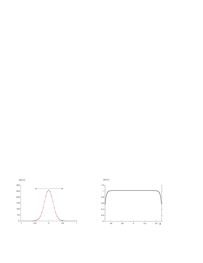
FIG. 3.: Equilibrium states for the gaussian potential (left: $T/T_{c}=0.9$, right: $T/T_{c}=1.1$); the length of the box is $L=100\xi$ and $N=100$ ($n_{0}=1$). On the left curve, the crosses are the results from the static algorithm whereas the solid line is the gaussian approximation defined below. $\xi$ is the unit length; note the different horizontal and vertical scales. Above the localized curve is shown the lenght $\xi$.

These calculations allow first to check the existence of the sharp transition occurring at $T_{\rm c}$ when the temperature is decreased starting with the uniform state; second, they reveal a hysteretic behaviour: when the temperature is increased starting from the localized state (one cluster), the transition from the localized state to the uniform one occurs at another temperature $T^{*}_{\rm c}\,>\,T_{\rm c}$.

Fig. 3 displays two typical density profiles (uniform vs localized cluster), just above and just below $T_{\rm c}$ obtained with this static algorithm. Since the width of the localized state turns out to be a little bit smaller than the range $\xi$ of the potential, the central part of the cluster can be safely approximated by a gaussian; indeed, when one expands the potential near $x/\xi\sim 0$, the harmonic potential is recovered (if instead of a gaussian potential, one chooses $v(x)=v_{0}{\rm e}^{-|x|/\xi}$, the central shape of the localized cluster is $1/\cosh^{2}x$, as it must (see (14)) since near the center this potential is essentially the Coulomb one). Obviously, such an approximation cannot properly represent the tails of the equilibrium density.

In order to characterize the transition, we introduce two quantities, $\varepsilon$ and $\lambda$ defined as follows:

$$\varepsilon(T/T_{\rm c})=\frac{1}{N}\int_{L}{\rm d}x\,{\rm d}x^{\prime}\,n(x)n(x^{\prime})v(x-x^{\prime})\enspace,$$ (51)

and:

$$\Delta^{2}(T/T_{\rm c})\,=\,\frac{1}{N}\int_{L}{\rm d}x\,x^{2}\,n(x)-\left[\frac{1}{N}\int_{L}{\rm d}x\,x\,n(x)\right]^{2}\enspace.$$ (52)

$\varepsilon$ represents the mean-field interaction energy per particle; $\Delta$ measures the spatial width of the cluster. For the uniform state one has $\varepsilon_{\rm unif}\,=\,(N/L)\int_{L}{{\rm d}x\,v(x)}\,\sim\,N(\xi/L)\,v_{0}$ and $\Delta_{\rm unif}\,\sim L\,\gg\xi$; on the contrary, for the localized state, $\varepsilon_{\rm loc}\,\sim\,N\,v_{0}$ and $\Delta_{\rm loc}\,\lesssim\,\xi$. For an infinite system, the ratio $\varepsilon_{\rm loc}/\varepsilon_{\rm uniform}$ vanishes, so that $\varepsilon$ can play the role of an order parameter.

The hysteresis is obtained as follows. For each given temperature, the starting point is the solution found in the previous run at a slightly different temperature. After a first sequence where $T/T_{\rm c}$ is decreased step by step down to $0.2$, the procedure is reversed, $T/T_{\rm c}$ is increased, the iterative procedure starting again from the localized solution obtained for the previous value of $T/T_{\rm c}$. It is found that the inverse transition does not occur at $T/T_{\rm c}=1$, but at a higher temperature $T_{\rm c}^{*}$.

Clearly, for $T<T_{\rm c}$, several solutions can exist. Since the width of the single peak solution is a bit smaller than the range $\xi$ of the potential, one can guess that there also exists a solution with two peaks separated by a distance much larger that $\xi$. This is confirmed by the numerical calculations: starting with a trial function having two separate peaks, the calculation converges towards a stable solution having the same features. One thus can claim that, on the low-temperature side, localized solutions exist displaying $j=1,\,2,\,3,\,\ldots$ peaks. Each of these solutions has its own temperature $T_{{\rm c},\,j}^{*}$. The corresponding typical hysteretic cycles are shown on figure (4) for the “order parameter” $\varepsilon$ for the one-,two-, and three-peak solutions.

The possibility of the $n$-peak solutions is confirmed by the dynamic algorithm (it was checked that the latter eventually yields the same equilibrium solutions as the static one). This allows to conclude that a given $j$-peak solution is linearly stable for $T_{\rm c}<T<T^{*}_{{\rm c},\,j}$. Note that the linear stability of the $n$-peak solutions above $T_{\rm c}$ is not in contradiction with the results obtained in section III; all this simply means that, in the region $T_{\rm c}<T<T^{*}_{{\rm c},\,j}$, both the uniform state and the localized state(s) are stable against small perturbations.

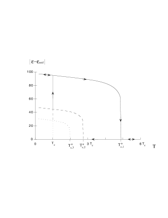
FIG. 4.: $|\varepsilon-\varepsilon_{\rm unif}|$ versus $T$: hysteresis cycle for the uniform-localized transition. Solid line: 1-peak branch, dashed line: 2-peak branch, dotted line: 3-peak branch.

Defining the entropy as $S=-\,\int_{L}{\rm d}x\,n(x)\,\ln[n(x)/n_{0}]$, it is seen that the one-peak solution is the one having the lowest free energy $F=\varepsilon-TS$. It must be noted that each kind of states has its own relevant physical parameters. For the uniform state, the relevant parameters are $v_{0},\xi,n_{0}=N/L$ and the critical temperature found by the linear stability analysis is a function of these parameters. For the localized state, the relevant parameters are $v_{0},\xi$ and $N$, the number of particles. Indeed, for this state, edge-effects become irrelevant when $\xi\ll L$: in this sense $L$ becomes arbitrary so that $n_{0}$ and $N$ are in fact independent variables.

The physical reason of the hysteresis can be understood as follows. In the uniform state, a given particle interacts with a small (microscopic) number of particles ($\sim n_{0}\xi$); on the contrary, in the localized state, a single particle interacts with a large number ($\sim N$), macroscopic in the sense that all the particles effectively interact with anyone of them (note that this also originates from the fact that the particles are of zero radius). The condition for the uniform-to-localized transition is expressed by $k_{\rm B}T_{\rm c}\,\sim\,n_{0}\xi|v_{0}|$ (see (40)). For the inverse transition, one can expect that a somewhat similar condition also holds true, so that $T_{\rm c}^{*}$ is an increasing function of $N$ (and is independent of $n_{0}$). It is likely that with pointlike particles $T_{\rm c}^{*}$ goes to infinity with $N$; on the contrary, with finite-size particles, one can figure out that $T_{\rm c}^{*}$ saturates at very large $N$. As a whole, the hysteretic behaviour is a consequence of this parameter cross-over between the two kinds of steady states.

These facts are illustrated by looking at the width $\Delta$ of the cluster in the localized state, displayed in fig. 5 where $\Delta$ is plotted as a function of the relevant variables for the uniform state (as they naturally arise in the linear stability analysis of section III). Indeed, choosing $N=50$ or $N=100$ with fixed $n_{0}$ gives two different curves.

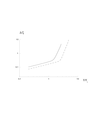
FIG. 5.: $\Delta$ versus $T/T_{\rm c}$, for $N=50$ (solid line), and $N=100$ (dashed line). The two curves display two well separated regimes; at low temperature, $\Delta\propto T^{1/2}$, whereas at high temperature, $\Delta$ still follows a power law, but with an exponent $\simeq 5.4$. Both curves end at their own localized-uniform transition temperature.

In the localized state, the width $\Delta$ of the cluster displays a cross-over between two regimes. On the low-$T$ side, one finds approximately $\Delta\propto T^{1/2}$. This behaviour is the same as for the harmonic case (see II B), which suggests that a gaussian approximation is valid in the low-$T$ region. Indeed, one can compare $\Delta$ with the analytic expression (18) obtained for the harmonic case (see figure 6). The agreement turns out to be quite good and this allows to claim that a gaussian approximation provides a very accurate description of the localized state arising in the low-$T$ region. For the second regime ($T_{\rm c}\,<\,T\,<\,T_{\rm c}^{*}$), the width of the cluster becomes of the same order or even greater than the potential range, so that the effective potential cannot be well represented by a harmonic approximation. Indeed, the increase of the cluster width with $T$ no more displays a gaussian behaviour, but still follows a power law.

FIG. 6.: Comparison between the gaussian approximation (dashed line) and the numerical results (solid line) for the dependence of the width vs the temperature, in the low-$T$ region ($N=100$).

V Dynamics of a system of particles interacting through the gaussian potential

In the previous mean-field analysis, it was shown that brownian particles interacting through a gaussian potential can have several steady states when $T_{\rm c}<T<T_{\rm c}^{*}$. The system will converge towards one of those states, depending of the initial condition. It can be expected that, under a strong perturbation, the former is able to shift from one steady state to another, without changing the two phase space parameters ($T/T_{\rm{c}}$ and $N$).

We here give a few results obtained with the dynamical algorithm for a set of $N=100$ particles starting in the uniform state at $T/T_{\rm{c}}=0.5$. The length of the box is $L=100\xi$. This represents a case where the system, being in its stable uniform state at a given $T>T_{\rm c}$, is cooled infinitely quickly below its critical temperature.

We find that the dynamics is a succession of steps, each of them being a metastable state. Each plateau has a free energy lower than that of the preceding. The mean energy per particle is plotted in fig. 7 as a function of time. In order to be complete, some corresponding density profiles at different times are shown in fig. 8.

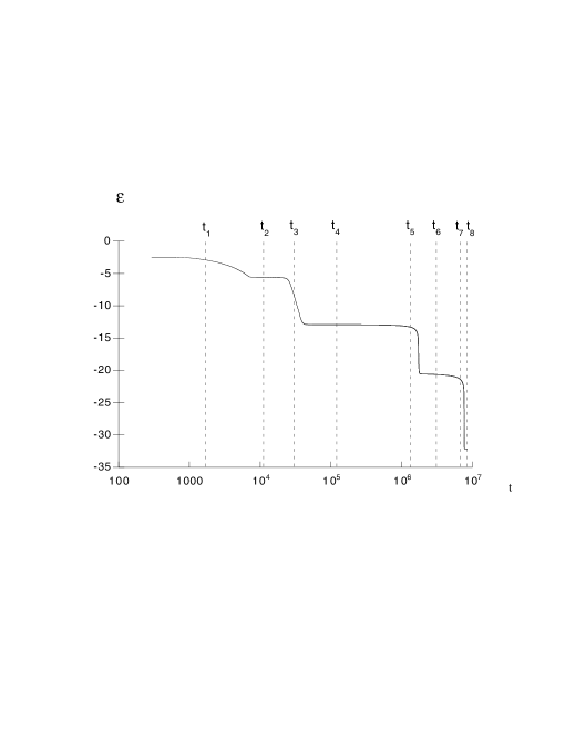
FIG. 7.: Time evolution of the mean energy per particle $\varepsilon$, starting with the uniform state sudenly cooled below the critical temperature ($T/T_{\rm c}=0.5$ and $N=100$). Note the horizontal logarithmic scale; the time unit is $\xi/(\mu n_{0}|v_{0}|)$.

These plots show that the dynamics is a succession of metastable states with a given number of peaks of high density, ($13$-peak state, $7$-peak state, $5$-peak state, $3$-peak state). The lifetime of these states rapidly increases when the number of peaks gets lower (note the horizontal logarithmic scale in fig. 7).

Because of computational time, we were unable to obtain the $1$-peak state. From static computations, it is believed that this state is expected to be the final one, although there is no evidence that the two algorithms have the same attraction basins. Moreover, the $1$-peak state is not the only stable state: we have checked that also exist stationary $2$-peak, and $3$-peak states, a fact which seems nearly obvious on physical grounds since when the distance between two neighbouring peaks is much larger that the range $\xi$ no dynamics can occur.

From the time-dependent density profiles (fig. 8), we see that “nucleation” always occurs at the boundaries of the box. This is easily understood, since a particle near this boundary is pulled from one side only, as opposed to a particle located in the bulk. This effect would disappear with periodic boundary conditions, indicating that the nucleation can only occur around an inhomogeneity.

It is also interesting to follow the annihilation of the peaks. As an example, one goes from $13$ to $7$-peaks via the diffusion of the even peaks into the odd ones. Generally speaking, it turns out that the transition towards a state having fewer peaks proceeds through the absorption of “weak” peaks into strong ones. The actual value of the density between the peaks, even when it is extremely small, turns out to be of first importance in this mechanism of coalescence.

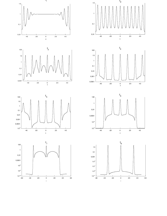
FIG. 8.: Sequence of the density profile at different times, starting from the uniform state cooled below $T_{\rm c}$.

VI Conclusion

In this paper, we have studied properties of the $N$-body Fokker-Planck equation within a mean field aproximation. Our aim was to analyse the properties of the steady state – which is a uniform density gas when interactions are set to zero – as a function of the features of the interaction potential. The linear stability analysis of the uniform state allowed to state the condition for a phase transition, as a result of the competing effects due to attractive interaction and to diffusive spreading. In particular, it was shown that the uniform phase is always unstable for non-summable attractive potentials, the critical temperature being infinite. In this latter case, analytical results have been given for specific potentials ($1d$-coulombian, harmonic, polynomials), all yielding an aggregated steady state.

For an attractive short ranged interaction, the above stability condition was interpreted as a phase transition occurring at a finite $T_{\rm c}$. This transition was more thoroughly studied by numerical computations in a definite case (gaussian potential) and turns out to be of the first order and hysteretic, the low temperature state being an inhomogeneous state having one or several peaks of high density.

The far-from-equilibrium dynamics was numerically computed for the gaussian potential, starting from the uniform state suddenly cooled below $T_{\rm c}$. The relaxation proceeds through a sequence of plateaux displaying a given decreasing number of peaks, each of the former having a longer and longer lifetime as time goes on. Each of these steps can be viewed as a metastable state.

Obviously enough, the considered problem requires further investigations. One of them is the relevance of mean field approach. If one expects that mean field results should be basically valid for long ranged potentials and high space dimensionality, their correctness for short range potential has to be checked by using more refined approximations from $N$-body general methods.

- [1] E.D. Williams, S.L. Cunningham, and W.H. Weinberg, A determination of adatom-adatom interaction energies : Application to oxygen chemisorbed on the tungsten (110) surface, J. Chem. Phys., 68, 4688 (1978)
- [2] W.Y. Ching, D.L. Huber, M. Fishkis, and M.G. Lagally, Monte Carlo modeling of phase changes in the chemisorption system O/W (110) , J. Vac. Sci., 15, 653 (1978)
- [3] M.C. Tringides, R. Gomer, A Monte Carlo study of oxygen diffusion on the (110) plane of tungsten , Surf. Sci., 145, 121 (1984)
- [4] R. Gomer, Diffusion of adsorbates on metal surfaces, Rep. Prog. Phys., 53, 917 (1990)
- [5] M.C. Tringides, R. Gomer, Adsorbate-adsorbate interaction effects in surface diffusion, Surf. Sci. , 265, 283 (1992)
- [6] M.A. Zaluska-Kotur, L.A. Turski, Diffusion coefficient for interacting lattice gases, Phys. Rev. B, 50, 16102 (1994)
- [7] Z.W. Gortel , M.A. Zaluska-Kotur, and L.A. Turski, Diffusion coefficient for interacting lattice gases : Repulsive interactions, Phys. Rev. B, 52, 16920 (1995)
- [8] W. Hess, R. Klein, Generalized hydrodynamics of systems of Brownian particles, Adv. Phys., 32, 173 (1983)
- [9] G. Nagele, M. Medina-Noyola, and R. Klein, Time-dependant self diffusion in model suspensions of highly charged Brownian particles, Physica A, 149, 123 (1988)
- [10] Cl. Aslangul Analytical study of an asymmetric 1D statistical model for chemical reactions, Physica A, 231, 687 (1996)
- [11] V. P. Zhdano, B. Kasemo, Kinetic phase transitions in simple reactions on solid surfaces, Surf. Sci. Rep., 20, 111 (1994)
- [12] K.W. Kehr, K. Binder, Simulation of diffusion in lattices gases and related kinetic phenomena in Applications of Monte Carlo methods in statistical physics, edited by K.Binder, Topics in current physics, vol. 36, p. 181 (Springer, Berlin, 1984)
- [13] C.W. Gardiner, Handbook of Stochastic Methods (Springer, 1990)
- [14] D. A. McQuarrie, Statistical Mechanics (Harper & Row, New York, 1973)
- [15] A. Erdelyi, W. Magnus, F. Oberhettinger and F. G. Tricomi, Tables of Integral Transforms, vol. I (McGrawHill, 1954)