Statistical Mechanics of Complex Networks

Abstract

Complex networks describe a wide range of systems in nature and society, much quoted examples including the cell, a network of chemicals linked by chemical reactions, or the Internet, a network of routers and computers connected by physical links. While traditionally these systems were modeled as random graphs, it is increasingly recognized that the topology and evolution of real networks is governed by robust organizing principles. Here we review the recent advances in the field of complex networks, focusing on the statistical mechanics of network topology and dynamics. After reviewing the empirical data that motivated the recent interest in networks, we discuss the main models and analytical tools, covering random graphs, small-world and scale-free networks, as well as the interplay between topology and the network’s robustness against failures and attacks.

CONTENTS

I INTRODUCTION

Complex weblike structures describe a wide variety of systems of high technological and intellectual importance. For example, the cell is best described as a complex network of chemicals connected by chemical reactions; the Internet is a complex network of routers and computers linked by various physical or wireless links; fads and ideas spread on the social network whose nodes are human beings and edges represent various social relationships; the Wold-Wide Web is an enormous virtual network of webpages connected by hyperlinks. These systems represent just a few of the many examples that have recently prompted the scientific community to investigate the mechanisms that determine the topology of complex networks. The desire to understand such interwoven systems has brought along significant challenges as well. Physics, a major beneficiary of reductionism, has developed an arsenal of successful tools to predict the behavior of a system as a whole from the properties of its constituents. We now understand how magnetism emerges from the collective behavior of millions of spins, or how do quantum particles lead to such spectacular phenomena as Bose-Einstein condensation or superfluidity. The success of these modeling efforts is based on the simplicity of the interactions between the elements: there is no ambiguity as to what interacts with what, and the interaction strength is uniquely determined by the physical distance. We are at a loss, however, in describing systems for which physical distance is irrelevant, or there is ambiguity whether two components interact. While for many complex systems with nontrivial network topology such ambiguity is naturally present, in the past few years we increasingly recognize that the tools of statistical mechanics offer an ideal framework to describe these interwoven systems as well. These developments have brought along new and challenging problems for statistical physics and unexpected links to major topics in condensed matter physics, ranging from percolation to Bose-Einstein condensation.

Traditionally the study of complex networks has been the territory of graph theory. While graph theory initially focused on regular graphs, since the 1950’s large-scale networks with no apparent design principles were described as random graphs, proposed as the simplest and most straightforward realization of a complex network. Random graphs were first studied by the Hungarian mathematicians Paul Erdős and Alfréd Rényi. According to the Erdős-Rényi (ER) model, we start with $N$ nodes and connect every pair of nodes with probability $p$, creating a graph with approximately $pN(N-1)/2$ edges distributed randomly. This model has guided our thinking about complex networks for decades after its introduction. But the growing interest in complex systems prompted many scientists to reconsider this modeling paradigm and ask a simple question: are real networks behind such diverse complex systems as the cell or the Internet, fundamentally random? Our intuition clearly indicates that complex systems must display some organizing principles which should be at some level encoded in their topology as well. But if the topology of these networks indeed deviates from a random graph, we need to develop tools and measures to capture in quantitative terms the underlying organizing principles.

In the past few years we witnessed dramatic advances in this direction, prompted by several parallel developments. First, the computerization of data acquisition in all fields led to the emergence of large databases on the topology of various real networks. Second, the increased computing power allows us to investigate networks containing millions of nodes, exploring questions that could not be addressed before. Third, the slow but noticeable breakdown of boundaries between disciplines offered researchers access to diverse databases, allowing them to uncover the generic properties of complex networks. Finally, there is an increasingly voiced need to move beyond reductionist approaches and try to understand the behavior of the system as a whole. Along this route, understanding the topology of the interactions between the components, i.e. networks, is unavoidable.

Motivated by these converging developments and circumstances, many quantities and measures have been proposed and investigated in depth in the past few years. However, three concepts occupy a prominent place in contemporary thinking about complex networks. Next we define and briefly discuss them, a discussion to be expanded in the coming chapters.

Small worlds: The small world concept in simple terms describes the fact that despite their often large size, in most networks there is a relatively short path between any two nodes. The distance between two nodes is defined as the number of edges along the shortest path connecting them. The most popular manifestation of ”small worlds” is the ”six degrees of separation” concept, uncovered by the social psychologist Stanley Milgram (1967), who concluded that there was a path of acquaintances with typical length about six between most pairs of people in the United States (Kochen 1989). The small world property appears to characterize most complex networks: the actors in Hollywood are on average within three costars from each other, or the chemicals in a cell are separated typically by three reactions. The small world concept, while intriguing, is not an indication of a particular organizing principle. Indeed, as Erdős and Rényi have demonstrated, the typical distance between any two nodes in a random graph scales as the logarithm of the number of nodes. Thus random graphs are small worlds as well.

Clustering: A common property of social networks is that cliques form, representing circles of of friends or acquaintances in which every member knows every other member. This inherent tendency to clustering is quantified by the clustering coefficient (Watts and Strogatz 1998). Let us focus first on a selected node $i$ in the network, having $k_{i}$ edges which connect it to $k_{i}$ other nodes. If the first neighbors of the original node were part of a clique, there would be $k_{i}(k_{i}-1)/2$ edges between them. The ratio between the number $E_{i}$ of edges that actually exist between these $k_{i}$ nodes and the total number $k_{i}(k_{i}-1)/2$ gives the value of the clustering coefficient of node $i$

$$C_{i}=\frac{2E_{i}}{k_{i}(k_{i}-1)}.$$ (1)

The clustering coefficient of the whole network is the average of all individual $C_{i}$’s.

In a random graph, since the edges are distributed randomly, the clustering coefficient is $C=p$ (Sect. III.F). However, it was Watts and Strogatz who first pointed out that in most, if not all, real networks the clustering coefficient is typically much larger than it is in a random network of equal number of nodes and edges.

Degree distribution: Not all nodes in a network have the same number of edges. The spread in the number of edges a node has, or node degree, is characterized by a distribution function $P(k)$, which gives the probability that a randomly selected node has exactly $k$ edges. Since in a random graph the edges are placed randomly, the majority of nodes have approximately the same degree, close to the average degree $\langle k\rangle$ of the network. The degree distribution of a random graph is a Poisson distribution with a peak at $P(\langle k\rangle)$. On the other hand recent empirical results show that for most large networks the degree distribution significantly deviates from a Poisson distribution. In particular, for a large number of networks, including the World-Wide Web (Albert, Jeong, Barabási 1999), Internet (Faloutsos et al. 1999) or metabolic networks (Jeong el al. 2000), the degree distribution has a power-law tail

$$P(k)\sim k^{-\gamma}.$$ (2)

Such networks are called scale-free (Barabási and Albert 1999). While some networks display an exponential tail, often the functional form of $P(k)$ still deviates significantly from a Poisson distribution expected for a random graph.

These three concepts, small path length, clustering and scale-free degree distribution have initiated a revival of network modeling in the past few years, resulting in the introduction and study of three main classes of modeling paradigms. First, random graphs, which are variants of the Erdős-Rényi model, are still widely used in many fields, and serve as a benchmark for many modeling and empirical studies. Second, following the discovery of clustering, a class of models, collectively called small world models, have been proposed. These models interpolate between the highly clustered regular lattices and random graphs. Finally, the discovery of the power-law degree distribution has led to the construction of various scale-free models that, by focusing on the network dynamics, aim to explain the origin of the power-law tails and other non-Poisson degree distributions seen in real systems.

The purpose of this article is to review each of these modeling efforts, focusing on the statistical mechanics of complex networks. Our main goal is to present the theoretical developments in parallel with the empirical data that initiated and support the various models and theoretical tools. To achieve this, we start with a brief description of the real networks and databases that represent the testground for most current modeling efforts.

II THE TOPOLOGY OF REAL NETWORKS: EMPIRICAL RESULTS

The study of most complex networks has been initiated by a desire to understand various real systems, ranging from communication networks to ecological webs. Thus the databases available for study span several disciplines. In this section we review briefly those that have been studied by researchers aiming to uncover the general features of complex networks. Beyond the description of the databases, we will focus on the three robust measures of the network topology: average path length, clustering coefficient and degree distribution. Other quantities, as discussed in the following chapters, will be again tested on these databases. The properties of the investigated databases, as well as the obtained exponents are summarized in Tables I and II.

1 World-Wide Web

The World-Wide Web (WWW) represents the largest network for which topological information is currently available. The nodes of the network are the documents (webpages) and the edges are the hyperlinks (URLs) that point from one document to another (see Fig 1). The size of this network was close to $1$ billion nodes at the end of 1999 (Lawrence and Giles 1998, 1999). The interest in the WWW as a network has boomed after it has been discovered that the degree distribution of the webpages follows a power-law over several orders of magnitude (Albert, Jeong, Barabási 1999, Kumaret al. 1999). Since the edges of the WWW are directed, the network is characterized by two degree distributions: the distribution of outgoing edges, $P_{out}(k)$, signifies the probability that a document has $k$ outgoing hyperlinks and the distribution of incoming edges, $P_{in}(k)$, is the probability that $k$ hyperlinks point to a certain document. Several studies have established that both $P_{out}(k)$ and $P_{in}(k)$ have power-law tails:

$$P_{out}(k)\sim k^{-\gamma_{out}}\quad\mbox{and}\quad P_{in}(k)\sim k^{-\gamma_{in}}.$$ (3)

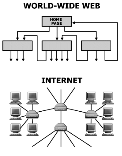
FIG. 1.: Network structure of the World-Wide Web and the Internet. Upper panel: the nodes of the World-Wide Web are web documents, connected with directed hyperlinks (URLs). Lower panel: on the Internet the nodes are the routers and computers, the edges are the wires and cables that physically connect them. Figure courtesy of István Albert.

Albert, Jeong and Barabási (1999) have studied a subset of the WWW containing $325,729$ nodes and have found $\gamma_{out}=2.45$ and $\gamma_{in}=2.1$. Kumar et al. (1999) used a $40$ million document crawl by Alexa Inc., obtaining $\gamma_{out}=2.38$ and $\gamma_{in}=2.1$ (see also Kleinberg et al. 1999). A later survey of the WWW topology by Broder et al. (2000) used two 1999 Altavista crawls containing in total $200$ million documents, obtaining $\gamma_{out}=2.72$ and $\gamma_{in}=2.1$ with scaling holding close to five orders of magnitude (Fig. 2). Adamic and Huberman (2000) used a somewhat different representation of the WWW, each node representing a separate domain name and two nodes being connected if any of the pages in one domain linked to any page in the other. While this method lumps together often thousands of pages that are on the same domain, representing a nontrivial aggregation of the nodes, the distribution of incoming edges still followed a power-law with $\gamma_{in}^{dom}=1.94$.

Note that $\gamma_{in}$ is the same for all measurements at the document level despite the two years time delay between the first and last web crawl, during which the WWW had grown at least five times larger. On the other hand, $\gamma_{out}$ has an increasing tendency with the sample size or time (see Table II).

Despite the large number of nodes, the WWW displays the small world property. This was first reported by Albert, Jeong and Barabási (1999), who found that the average path length for a sample of $325,729$ nodes was $11.2$ and predicted, using finite size scaling, that for the full WWW of $800$ million nodes that would be around $19$. Subsequent measurements of Broder et al. (2000) found that the average path length between nodes in a $200$ million sample of the WWW is $16$, in agreement with the finite size prediction for a sample of this size. Finally, the domain level network displays an average path length of $3.1$ (Adamic 1999).

The directed nature of the WWW does not allow us to measure the clustering coefficient using Eq. (1). One way to avoid this difficulty is to make the network undirected, making each edge bidirectional. This was the path followed by Adamic (1999) who studied the WWW at the domain level using an 1997 Alexa crawl of $50$ million webpages distributed between $259,794$ sites. Adamic removed the nodes which have only one edge, focusing on a network of $153,127$ sites. While these modifications are expected to increase somewhat the clustering coefficient, she found $C=0.1078$, orders of magnitude higher than $C_{rand}=0.00023$ corresponding to a random graph of the same size and average degree.

FIG. 2.: Degree distribution of the World-Wide Web from two different measurements. Squares correspond to the $325,729$ sample of Albert et al. (1999), and circles represent the measurements of over a $200$ million pages by Broder et al. (2000) (courtesy of Altavista and Andrew Tomkins). (a) Degree distribution of the outgoing edges. (b) Degree distribution of the incoming edges. The data has been binned logarithmically to reduce noise.

2 Internet

The Internet is the network of the physical links between computers and other telecommunication devices (Fig. 1). The topology of the Internet is studied at two different levels. At the router level the nodes are the routers, and edges are the physical connections between them. At the interdomain (or autonomous system) level each domain, composed of hundreds of routers and computers, is represented by a single node, and an edge is drawn between two domains if there is at least one route that connects them. Faloutsos et al. (1999) have studied the Internet at both levels, concluding that in each case the degree distribution follows a power-law. The interdomain topology of the Internet, captured at three different dates between $1997$ and the end of $1998$, resulted in degree exponents between $\gamma_{I}^{as}=2.15$ and $\gamma_{I}^{as}=2.2$. The $1995$ survey of the Internet topology at the router level, containing $3,888$ nodes found $\gamma_{I}^{r}=2.48$ (Faloutsos et al. 1999). Recently Govindan and Tangmunarunkit (2000) mapped the connectivity of nearly $150,000$ router interfaces and nearly $200,000$ router adjacencies, confirming the power-law scaling with $\gamma_{I}^{r}\simeq 2.3$ (see Fig. 3a).

FIG. 3.: The degree distribution of several real networks. (a) Internet at the router level. Data courtesy of Ramesh Govindan. (b) Movie actor collaboration network (after Barabási and Albert 1999). Note that if TV series are included as well, which aggregate a large number of actors, an exponential cutoff emerges for large $k$ (Amaral et al. 2000). (c) Coauthorship network of high energy physicists (after Newman 2001a,b). (d) Coauthorship network of neuroscientists (after Barabási et al. 2001).

The Internet as a network does display clustering and small path length as well. Yook et al. (2001a) and Pastor-Satorras et al. (2001), studying the Internet at the domain level between 1997 and 1999 have found that its clustering coefficient ranged between $0.18$ and $0.3$, to be compared with $C_{rand}\simeq 0.001$ for random networks of similar parameters. The average path length of the Internet at the domain level ranged between $3.70$ and $3.77$ (Yook et al. 2001a, Pastor-Satorras et al. 2001), and at the router level it was around $9$ (Yook et al. 2001a), indicating its small world character.

3 Movie actor collaboration network

A much studied database is the movie actor collaboration network, based on the Internet Movie Database that contains all movies and their casts since the 1890’s. In this network the nodes are the actors, and two nodes have a common edge if the corresponding actors have acted in a movie together. This is a continuously expanding network, with $225,226$ nodes in 1998 (Watts, Strogatz 1998) which grew to $449,913$ nodes by May 2000 (Newman, Strogatz and Watts 2000). The average path length of the actor network is close to that of a random graph with the same size and average degree, $3.65$ compared to $2.9$, but its clustering coefficient is more than $100$ times higher than a random graph (Watts and Strogatz 1998). The degree distribution of the movie actor network has a power-law tail for large $k$ (see Fig. 3b), following $P(k)\sim k^{-\gamma_{actor}}$, where $\gamma_{actor}=2.3\pm 0.1$ (Barabási and Albert 1999, Amaral et al. 2000, Albert and Barabási 2000).

4 Science collaboration graph

A collaboration network similar to that of the movie actors can be constructed for scientists, where the nodes are the scientists and two nodes are connected if the two scientists have written an article together. To uncover the topology of this complex graph, Newman (2001a,b,c) studied four databases spanning physics, biomedical research, high-energy physics and computer science over a 5 year window (1995-1999). All these networks show small average path length but high clustering coefficient, as summarized in Table I. The degree distribution of the collaboration network of high-energy physicists is an almost perfect power-law with an exponent of $1.2$ (Fig. 3c), while the other databases display power-laws with a larger exponent in the tail.

Barabási et al. 2001 investigated the collaboration graph of mathematicians and neuroscientists publishing between 1991 and 1998. The average path length of these networks is around $\ell_{math}=9.5$ and $\ell_{nsci}=6$, their clustering coefficient being $C_{math}=0.59$ and $C_{nsci}=0.76$. The degree distributions of these collaboration networks are consistent with power-laws with degree exponents $2.1$ and $2.5$, respectively (see Fig. 3d).

5 The web of human sexual contacts

Many sexually transmitted diseases, including AIDS, spread on a network of sexual relationships. Liljeros et al. (2001) have studied the web constructed from the sexual relations of $2810$ individuals, based on an extensive survey conducted in Sweden in 1996. Since the edges in this network are relatively short lived, they analyzed the distribution of partners over a single year, obtaining both for females and males a power-law degree distribution with an exponent $\gamma_{f}=3.5\pm 0.2$ and $\gamma_{m}=3.3\pm 0.2$, respectively.

6 Cellular networks

Jeong et al. (2000) studied the metabolism of $43$ organisms representing all three domains of life, reconstructing them in networks in which the nodes are the substrates (such as ATP, ADP, $\rm{H_{2}O}$) and the edges represent the predominantly directed chemical reactions in which these substrates can participate. The distribution of the outgoing and incoming edges have been found to follow power-laws for all organisms, the degree exponents varying between $2.0$ and $2.4$. While due to the network’s directedness the clustering coefficient has not been determined, the average path length was found to be approximately the same in all organisms, with a value of $3.3$.

The clustering coefficient was studied by Wagner and Fell (2000, see also Fell and Wagner 2000), focusing on the energy and biosynthesis metabolism of the Escherichia Coli bacterium, finding that, in addition to the power-law degree distribution, the undirected version of this substrate graph has small average path length and large clustering coefficient (see Table I).

Another important network characterizing the cell describes protein-protein interactions, where the nodes are proteins and they are connected if it has been experimentally demonstrated that they bind together. A study of these physical interactions shows that the degree distribution of the physical protein interaction map for yeast follows a power-law with an exponential cutoff $P(k)\sim(k+k_{0})^{-\gamma}e^{-(k+k_{0})/k_{c}}$ with $k_{0}=1$, $k_{c}=20$ and $\gamma=2.4$ (Jeong et al. 2001).

7 Ecological networks

Food webs are used regularly by ecologists to quantify the interaction between various species (Pimm 1991). In a food web the nodes are species and the edges represent predator-prey relationships between them. In a recent study, Williams et al. (2000) investigated the topology of the seven most documented and largest food webs, such as the Skipwith Pond, Little Rock Lake, Bridge Brook Lake, Chesapeake Bay, Ythan Estuary, Coachella Valley and St. Martin Island webs. While these webs differ widely in the number of species or their average degree, they all indicate that species in habitats are three or fewer edges from each other. This result was supported by the independent investigations of Montoya and Solé (2000) and Camacho et al. (2001a), who have shown that food webs are highly clustered as well. The degree distribution was first addressed by Montoya and Solé (2000), focusing on the Ythan Estuary, Silwood Park and Little Rock Lake food webs, considering these networks as being nondirected. Although the size of these webs is small (the largest of them has $N=186$ nodes), they appear to share the non-random properties of their larger counterparts. In particular, Montoya and Solé (2000) concluded that the degree distribution is consistent with a power-law with an unusually small exponent of $\gamma\simeq 1.1$. The small size of these webs does give room, however, for some ambiguity in $P(k)$. Camacho et al. (2001a,b) find that for some food webs an exponential fit works equally well. While the well documented existence of keystone species that play an important role in the food web topology points towards the existence of hubs (a common feature of scale-free networks), an unambiguous determination of the network’s topology could benefit from larger datasets. Due to the inherent difficulty in the data collection process (Williams et al. 2000), this is not expected anytime soon.

8 Phone-call network

A large directed graph has been constructed from the long distance telephone call patterns, where nodes are phone numbers and every completed phone call is an edge, directed from the caller to the receiver. Abello, Pardalos and Resende (1999) and Aiello, Chung and Lu (2000) studied the call graph of long distance telephone calls made during a single day, finding that the degree distribution of the outgoing and incoming edges follow a power-law with exponent $\gamma_{out}=\gamma_{in}=2.1$.

9 Citation networks

A rather complex network is formed by the citation patterns of scientific publications, the nodes standing for published articles and a directed edge representing a reference to a previously published article. Redner (1998), studying the citation distribution of $783,339$ papers cataloged by the Institute of Scientific Information, and of the $24,296$ papers published in Physical Review D between $1975$ and $1994$, has found that the probability that a paper is cited $k$ times follows a power-law with exponent $\gamma_{cite}=3$, indicating that the incoming degree distribution of the citation network follows a power-law. A recent study of Vázquez (2001) extended these studies to the outgoing degree distribution as well, obtaining that it has an exponential tail.

10 Networks in linguistics

The complexity of human languages offers several possibilities to define and study complex networks. Recently Ferrer i Cancho and Solé (2001) have constructed such a network for the English language, based on the British National Corpus, words, as nodes, being linked if they appear next or one word apart from each other in sentences. They have found that the resulting network of $440,902$ words displays a small average path length $\ell=2.67$, a high clustering coefficient $C=0.437$, and a two-regime power-law degree distribution. Words with degree $k\leq 10^{3}$ decay with a degree exponent $\gamma_{<}=1.5$ while words with $10^{3}<k<10^{5}$ follow a power-law with $\gamma_{>}\simeq 2.7$.

A different study (Yook, Jeong, Barabási 2001b) linked words based on their meaning, i.e. two words were connected to each other if they were known to be synonyms according to the Merriam-Webster Dictionary. The results indicate the existence of a giant cluster of $22,311$ words from the total of $23,279$ words which have synonyms, with an average path length $\ell=4.5$, and a rather high clustering coefficient $C=0.7$ compared to $C_{rand}=0.0006$ for an equivalent random network. In addition the degree distribution followed had a power-law tail with $\gamma_{syn}=2.8$. These results indicate that in many respects the language also forms a complex network with organizing principles not so different from the examples discussed earlier (see also Steyvers and Tennenbaum 2001).

11 Power and neural networks

The power grid of the western United States is described by a complex network whose nodes are generators, transformers and substations, and the edges are high-voltage transmission lines. The number of nodes in the power grid is $N=4,941$, and $\langle k\rangle=2.67$. In the tiny ($N=282$) neural network of the nematode worm C. elegans, the nodes are the neurons, and an edge joins two neurons if they are connected by either a synapse or a gap junction. Watts and Strogatz (1998) found that while for both networks the average path length was approximately equal with that of a random graph with the same size and average degree, their clustering coefficient was much higher (Table I). The degree distribution of the power grid is consistent with an exponential, while for the neural network it has a peak at an intermediate $k$ after which it decays following an exponential (Amaral et al. 2000).

12 Protein folding

During folding a protein takes up consecutive conformations. Representing with a node each distinct state, two conformations are linked if they can be obtained from each other by an elementary move. Scala et al. (2000) studied the network formed by the conformations of a 2D lattice polymer, obtaining that it has small-world properties. Specifically, the average path length increases logarithmically when the size of the polymer (and consequently the size of the network) increases, similarly to the behavior seen in a random graph. The clustering coefficient, however, is much larger than $C_{rand}$, a difference that increases with the network size. The degree distribution of this conformation network is consistent with a gaussian (Amaral et al. 2000).

The databases discussed above served as motivation and source of inspiration for uncovering the topological properties of real networks. We will refer to them frequently to validate various theoretical predictions, or to understand the limitations of the modeling efforts. In the remaining of the review we discuss the various theoretical tools developed to model these complex networks. In this respect, we need to start with the mother of all network models: the random graph theory of Erdős and Rényi.

TABLE I.: The general characteristics of several real networks. For each network we indicated the number of nodes, the average degree $\langle k\rangle$, the average path length $\ell$ and the clustering coefficient $C$. For a comparison we have included the average path length $\ell_{rand}$ and clustering coefficient $C_{rand}$ of a random graph with the same size and average degree. The last column identifies the symbols in Figs. 8 and 9.

Network	Size	$\langle k\rangle$	$\ell$	$\ell_{rand}$	$C$	$C_{rand}$	Reference	Nr.
WWW, site level, undir.	$153,127$	$35.21$	$3.1$	$3.35$	$0.1078$	$0.00023$	Adamic 1999	1
Internet, domain level	$3015$ - $6209$	$3.52$ - $4.11$	$3.7$ - $3.76$	$6.36$ - $6.18$	$0.18$ - $0.3$	$0.001$	Yook et al. 2001a,
							Pastor-Satorras et al. 2001	2
Movie actors	$225,226$	$61$	$3.65$	$2.99$	$0.79$	$0.00027$	Watts, Strogatz 1998	3
LANL coauthorship	$52,909$	$9.7$	$5.9$	$4.79$	$0.43$	$1.8\times 10^{-4}$	Newman 2001a,b	4
MEDLINE coauthorship	$1,520,251$	$18.1$	$4.6$	$4.91$	$0.066$	$1.1\times 10^{-5}$	Newman 2001a,b	5
SPIRES coauthorship	$56,627$	$173$	$4.0$	$2.12$	$0.726$	$0.003$	Newman 2001a,b,c	6
NCSTRL coauthorship	$11,994$	$3.59$	$9.7$	$7.34$	$0.496$	$3\times 10^{-4}$	Newman 2001a,b	7
Math coauthorship	$70,975$	$3.9$	$9.5$	$8.2$	$0.59$	$5.4\times 10^{-5}$	Barabási et al. 2001	8
Neurosci. coauthorship	$209,293$	$11.5$	$6$	$5.01$	$0.76$	$5.5\times 10^{-5}$	Barabási et al. 2001	9
E. coli, substrate graph	$282$	$7.35$	$2.9$	$3.04$	$0.32$	$0.026$	Wagner, Fell 2000	10
E. coli, reaction graph	$315$	$28.3$	$2.62$	$1.98$	$0.59$	$0.09$	Wagner, Fell 2000	11
Ythan estuary food web	$134$	$8.7$	$2.43$	$2.26$	$0.22$	$0.06$	Montoya, Solé 2000	12
Silwood park food web	$154$	$4.75$	$3.40$	$3.23$	$0.15$	$0.03$	Montoya, Solé 2000	13
Words, cooccurence	$460.902$	$70.13$	$2.67$	$3.03$	$0.437$	$0.0001$	Cancho, Solé 2001	14
Words, synonyms	$22,311$	$13.48$	$4.5$	$3.84$	$0.7$	$0.0006$	Yook et al. 2001	15
Power grid	$4,941$	$2.67$	$18.7$	$12.4$	$0.08$	$0.005$	Watts, Strogatz 1998	16
C. Elegans	$282$	$14$	$2.65$	$2.25$	$0.28$	$0.05$	Watts, Strogatz 1998	17

TABLE II.: The scaling exponents characterizing the degree distribution of several scale-free networks, for which $P(k)$ follows a power-law (2). We indicate the size of the network, its average degree $\langle k\rangle$ and the cutoff $\kappa$ for the power-law scaling. For directed networks we list separately the indegree ($\gamma_{in}$) and outdegree ($\gamma_{out}$) exponents, while for the undirected networks, marked with a star, these values are identical. The columns $l_{real}$, $l_{rand}$ and $l_{pow}$ compare the average path length of real networks with power-law degree distribution and the prediction of random graph theory (17) and that of Newman, Strogatz and Watts (2000) (62), as discussed in Sect. V. The last column identifies the symbols in Figs. 8 and 9.

Network	Size	$\langle k\rangle$	$\kappa$	$\gamma_{out}$	$\gamma_{in}$	$\ell_{real}$	$\ell_{rand}$	$\ell_{pow}$	Reference	Nr.
WWW	$325,729$	$4.51$	$900$	$2.45$	$2.1$	$11.2$	$8.32$	$4.77$	Albert, Jeong, Barabási 1999	1
WWW	$4\times 10^{7}$	$7$		$2.38$	$2.1$				Kumar et al. 1999	2
WWW	$2\times 10^{8}$	$7.5$	$4,000$	$2.72$	$2.1$	$16$	$8.85$	$7.61$	Broder et al. 2000	3
WWW, site	$260,000$				$1.94$				Huberman, Adamic 2000	4
Internet, domain$*$	$3,015$ - $4,389$	$3.42$ - $3.76$	$30-40$	$2.1$ - $2.2$	$2.1$ - $2.2$	$4$	$6.3$	$5.2$	Faloutsos 1999	5
Internet, router$*$	$3,888$	$2.57$	$30$	$2.48$	$2.48$	$12.15$	$8.75$	$7.67$	Faloutsos 1999	6
Internet, router$*$	$150,000$	$2.66$	$60$	$2.4$	$2.4$	$11$	$12.8$	$7.47$	Govindan 2000	7
Movie actors$*$	$212,250$	$28.78$	$900$	$2.3$	$2.3$	$4.54$	$3.65$	$4.01$	Barabási, Albert 1999	8
Coauthors, SPIRES$*$	$56,627$	$173$	$1,100$	$1.2$	$1.2$	$4$	$2.12$	$1.95$	Newman 2001b,c	9
Coauthors, neuro.$*$	$209,293$	$11.54$	$400$	$2.1$	$2.1$	$6$	$5.01$	$3.86$	Barabási et al. 2001	10
Coauthors, math$*$	$70,975$	$3.9$	$120$	$2.5$	$2.5$	$9.5$	$8.2$	$6.53$	Barabási et al. 2001	11
Sexual contacts$*$	$2810$			$3.4$	$3.4$				Liljeros et al. 2001	12
Metabolic, E. coli	$778$	$7.4$	$110$	$2.2$	$2.2$	$3.2$	$3.32$	$2.89$	Jeong et al. 2000	13
Protein, S. cerev.$*$	$1870$	$2.39$		$2.4$	$2.4$				Mason et al. 2000	14
Ythan estuary$*$	$134$	$8.7$	$35$	$1.05$	$1.05$	$2.43$	$2.26$	$1.71$	Montoya, Solé 2000	14
Silwood park$*$	$154$	$4.75$	$27$	$1.13$	$1.13$	$3.4$	$3.23$	$2$	Montoya, Solé 2000	16
Citation	$783,339$	$8.57$			$3$				Redner 1998	17
Phone-call	$53\times 10^{6}$	$3.16$		$2.1$	$2.1$				Aiello et al. 2000	18
Words, cooccurence$*$	$460,902$	$70.13$		$2.7$	$2.7$				Cancho, Solé 2001	19
Words, synonyms$*$	$22,311$	$13.48$		$2.8$	$2.8$				Yook et al. 2001	20

III RANDOM GRAPH THEORY

In mathematical terms a network is represented by a graph. A graph is a pair of sets $G=\{P,E\}$, where $P$ is a set of $N$ nodes (or vertices or points) $P_{1}$, $P_{2}$, .. $P_{N}$ and $E$ is a set of edges (or links or lines) that connect two elements of $P$. Graphs are usually represented as a set of dots, each corresponding to a node, two of these dots being joined by a line if the corresponding nodes are connected (see Fig. 4).

FIG. 4.: Illustration of a graph with $N=5$ nodes and $n=4$ edges. The set of the nodes is $P=\{1,2,3,4,5\}$ and the edge set is $E=\{\{1,2\},\{1,5\},\{2,3\},\{2,5\}\}$.

Graph theory has its origins in the $18$th century in the work of Leonhard Euler, the early work concentrating on small graphs with a high degree of regularity. In the $20$th century graph theory has become more statistical and algorithmic. A particularly rich source of ideas has been the study of random graphs, graphs in which the edges are distributed randomly. Networks with a complex topology and unknown organizing principles often appear random, thus random graph theory is regularly used in the study of complex networks.

The theory of random graphs was founded by Paul Erdős and Alfréd Rényi (1959,1960,1961), after Erdős discovered that probabilistic methods were often useful in tackling problems in graph theory. An detailed review of the field is available in the classic book of Bollobás (1985), complemented by the review of the parallels between phase transitions and random graph theory of Cohen (1988), and the guide of the history of the Erdős-Rényi approach by Karoński and Rućinski (1997). In the following we briefly describe the most important results of random graph theory, focusing on the aspects that are of direct relevance to complex networks.

A The Erdős-Rényi model

In their classic first article on random graphs, Erdős and Rényi define a random graph as $N$ labeled nodes connected by $n$ edges which are chosen randomly from the $\frac{N(N-1)}{2}$ possible edges (Erdős and Rényi 1959). In total there are $C_{\frac{N(N-1)}{2}}^{\,n}$ graphs with $N$ nodes and $n$ edges, forming a probability space in which every realization is equiprobable.

An alternative and equivalent definition of a random graph is called the binomial model. Here we start with $N$ nodes, every pair of nodes being connected with probability $p$ (see Fig. 5). Consequently, the total number of edges is a random variable with the expectation value $E(n)=p\frac{N(N-1)}{2}$. If $G_{0}$ is a graph with nodes $P_{1}$, $P_{2}$, .. $P_{N}$ and $n$ edges, the probability of obtaining it by this graph construction process is $P(G_{0})=p^{n}(1-p)^{\frac{N(N-1)}{2}-n}$.

Random graph theory studies the properties of the probability space associated with graphs with $N$ nodes as $N\rightarrow\infty$. Many properties of such random graphs can be determined using probabilistic arguments. In this respect Erdős and Rényi used the definition that almost every graph has a property $Q$ if the probability of having $Q$ approaches $1$ as $N\rightarrow\infty$. Among the questions addressed by Erdős and Rényi some have direct relevance to understanding complex networks as well, such as: Is a typical graph connected? Does it contain a triangle of connected nodes? How does its diameter depend on its size?

FIG. 5.: Illustration of the graph evolution process for the Erdős-Rényi model. We start with $N=10$ isolated nodes (upper panel), then connect every pair of nodes with probability $p$. The lower panel of the figure shows two different stages in the graph’s development, corresponding to $p=0.1$ and $p=0.15$. We can notice the emergence of trees (a tree of order $3$, drawn with dashed lines) and cycles (a cycle of order $3$, drawn with dotted lines) in the graph, and a connected cluster which unites half of the nodes at $p=0.15=1.5/N$.

The construction of a random graph is often called in the mathematical literature an evolution: starting with a set of $N$ isolated vertices, the graph develops by the successive addition of random edges. The graphs obtained at different stages of this process correspond to larger and larger connection probabilities $p$, eventually obtaining a fully connected graph (having the maximum number of edges $n=N(N-1)/2$) for $p\rightarrow 1$. The main goal of random graph theory is to determine at what connection probability $p$ will a particular property of a graph most likely arise. The greatest discovery of Erdős and Rényi was that many important properties of random graphs appear quite suddenly. That is, at a given probability either almost every graph has the property $Q$ (e.g. every pair of nodes is connected by a path of consecutive edges) or on the contrary, almost no graph has it. The transition from a property being very unlikely to being very likely is usually swift. For many such properties there is a critical probability $p_{c}(N)$. If $p(N)$ grows slower than $p_{c}(N)$ as $N\rightarrow\infty$, then almost every graph with connection probability $p(N)$ fails to have $Q$. If $p(N)$ grows somewhat faster than $p_{c}(N)$, then almost every graph has the property $Q$. Thus the probability that a graph with $N$ nodes and connection probability $p=p(N)$ has property $Q$ satisfies

$$\lim_{N\rightarrow\infty}P_{N,\,p}(Q)=\left\{\begin{array}[]{rcl}0&\mbox{if}&\frac{p(N)}{p_{c}(N)}\rightarrow 0\\ 1&\mbox{if}&\frac{p(N)}{p_{c}(N)}\rightarrow\infty\end{array}\right..$$ (4)

An important note is in order here. Physicists trained in critical phenomena will recognize in $p_{c}(N)$ the critical probability familiar in percolation. In the physics literature usually the system is viewed at a fixed system size $N$ and then the different regimes in (4) reduce to the question whether $p$ is smaller or larger than $p_{c}$. The proper value of $p_{c}$, that is, the limit $p_{c}=p_{c}(N\rightarrow\infty)$ is obtained by finite size scaling. The basis of this procedure is the assumption that this limit exists, reflecting the fact that ultimately the percolation threshold is independent of the system size. This is usually the case in finite dimensional systems which include most physical systems of interest for percolation theory and critical phenomena. In contrast, networks are, by definition, infinite dimensional: the number of neighbors a node can have increases linearly with the system size. Consequently, in random graph theory the occupation probability is defined as a function of the system size: $p$ represents the fraction of the edges which are present from the possible $N(N-1)/2$. Larger graphs with the same $p$ will contain more edges, and consequently properties like the appearance of cycles could occur for smaller $p$ in large graphs than in smaller ones. This means that for many properties $Q$ in random graphs there is no unique, $N$-independent threshold, but we have to define a threshold function which depends on the system size, and $p_{c}(N\rightarrow\infty)\rightarrow 0$. On the other hand, we will see that the average degree of the graph

$$\langle k\rangle=2n/N=p(N-1)\simeq pN$$ (5)

does have a critical value which is independent of the system size. In the coming subsection we illustrate these ideas by looking at the emergence of various subgraphs in random graphs.

B Subgraphs

The first property of random graphs studied by Erdős and Rényi (1959) was the appearance of subgraphs. A graph $G_{1}$ consisting of a set $P_{1}$ of nodes and a set $E_{1}$ of edges is a subgraph of a graph $G=\{P,E\}$ if all nodes in $P_{1}$ are also nodes of $P$ and all edges in $E_{1}$ are also edges of $E$. The simplest examples of subgraphs are cycles, trees and complete subgraphs (see Fig. 5). A cycle of order $k$ is a closed loop of $k$ edges such that every two consecutive edges and only those have a common node. That is, graphically a triangle is a cycle of order 3, while a rectangle is a cycle of order 4. The average degree of a cycle is equal to $2$, since every node has two edges. The opposite of closed loops are the trees, which cannot form closed loops. More precisely, a graph is a tree of order $k$ if it has $k$ nodes and $k-1$ edges, and none of its subgraphs is a cycle. The average degree of a tree of order $k$ is $\langle k\rangle=2-2/k$, approaching $2$ for large trees. Complete subgraphs of order $k$ contain $k$ nodes and all the possible $k(k-1)/2$ edges, in other words being completely connected.

Let us consider the evolution process described in Fig. 5 for a graph $G=G_{N,p}$. We start from $N$ isolated nodes, then connect every pair of nodes with probability $p$. For small connection probabilities the edges are isolated, but as $p$, and with it the number of edges, increases, two edges can attach at a common node, forming a tree of order $3$. An interesting problem is to determine the critical probability $p_{c}(N)$ at which almost every graph $G$ contains a tree of order $3$. Most generally we can ask whether there is a critical probability which marks the appearance of arbitrary subgraphs consisting of $k$ nodes and $l$ edges.

In random graph theory there is a rigorously proven answer to this question (Bollobás 1985). Consider a random graph $G=G_{N,p}$. In addition, consider a small graph $F$ consisting of $k$ nodes and $l$ edges. In principle, the random graph $G$ can contain several such subgraphs $F$. Our first goal is to determine how many such subgraphs exist. The $k$ nodes can be chosen from the total number of nodes $N$ in $C_{N}^{k}$ ways and the $l$ edges are formed with probability $p^{l}$. In addition, we can permute the $k$ nodes and potentially obtain $k!$ new graphs (the correct value is $k!/a$, where $a$ is the number of graphs which are isomorphic to each other). Thus the expected number of subgraphs $F$ contained in $G$ is

$$E(X)=C_{N}^{k}\frac{k!}{a}p^{l}\simeq\frac{N^{k}p^{l}}{a}.$$ (6)

This notation suggests that the actual number of such subgraphs, $X$, can be different from $E(X)$, but in the majority of the cases it will be close to it. Note that the subgraphs do not have to be isolated, i.e. there can exist edges with one of their nodes inside the subgraph, but the other outside of it.

Equation (6) indicates that if $p(N)$ is such that $p(N)N^{k/l}\rightarrow 0$ as $N\rightarrow 0$, the expected number of subgraphs $E(X)\rightarrow 0$, i.e. almost none of the random graphs contains a subgraph $F$. On the other hand, if $p(N)=cN^{-k/l}$, the mean number of subgraphs is a finite number, denoted by $\lambda=c^{l}/a$, indicating that this function might be the critical probability. The validity of this finding can be tested by calculating the distribution of subgraph numbers, $P_{p}(X=r)$, obtaining (Bollobás 1995)

$$\lim_{N\rightarrow\infty}P_{p}(X=r)=e^{-\lambda}\frac{\lambda^{r}}{r!}.$$ (7)

The probability that $G$ contains at least one subgraph $F$ is then

$$P_{p}(G\supset F)=\sum_{r=1}^{\infty}P_{p}(X=r)=1-e^{-\lambda},$$ (8)

which converges to $1$ as $c$ increases. For $p$ values satisfying $pN^{k/l}\rightarrow\infty$ the probability $P_{p}(G\supset F)$ converges to $1$, thus, indeed, the critical probability at which almost every graph contains a subgraph with $k$ nodes and $l$ edges is $p_{c}(N)=cN^{-k/l}$.

A few important special cases directly follow from Eq. (8):

(a) The critical probability of having a tree of order $k$ is $p_{c}(N)=cN^{-k/(k-1)}$;

(b) The critical probability of having a cycle of order $k$ is $p_{c}(N)=cN^{-1}$;

(c) The critical probability of having a complete subgraph of order $k$ is $p_{c}(N)=cN^{-2/(k-1)}$.

C Graph Evolution

It is instructive to view the results discussed above from a different point of view. Consider a random graph with $N$ nodes and assume that the connection probability $p(N)$ scales as $N^{z}$, where $z$ is a tunable parameter that can take any value between $-\infty$ and $0$ (Fig. 6). For $z$ less than $-3/2$ almost all graphs contain only isolated nodes and edges. When $z$ passes through $-3/2$, trees of order $3$ suddenly appear. When $z$ reaches $-4/3$, trees of order $4$ appear, and as $z$ approaches $-1$, the graph contains trees of larger and larger order. However, as long as $z<-1$, such that the average degree of the graph $\langle k\rangle=pN\rightarrow 0$ as $N\rightarrow\infty$, the graph is a union of disjoint trees, and cycles are absent. Exactly when $z$ passes through $-1$, corresponding to $\langle k\rangle=$const, even though $z$ is changing smoothly, the asymptotic probability of cycles of all orders jumps from $0$ to $1$. Cycles of order $3$ can be also viewed as complete subgraphs of order $3$. Complete subgraphs of order $4$ appear at $z=-2/3$, and as $z$ continues to increase, complete subgraphs of larger and larger order continue to emerge. Finally, as $z$ approaches $0$, almost every random graph approaches the complete graph of $N$ points.

FIG. 6.: The threshold probabilities at which different subgraphs appear in a random graph. For $pN^{3/2}\rightarrow 0$ the graph consists of isolated nodes and edges. For $p\sim N^{-3/2}$ trees of order $3$ appear, at $p\sim N^{-4/3}$ trees of order $4$. At $p\sim N^{-1}$ trees of all orders are present, and in the same time cycles of all orders appear. The probability $p\sim N^{-2/3}$ marks the appearance of complete subgraphs of order $4$ and $p\sim N^{-1/2}$ corresponds to complete subgraphs of order $5$. As $z$ approaches $0$, the graph contains complete subgraphs of increasing order.

Further results can be derived for $z=-1$, i.e. when we have $p\propto N^{-1}$ and the average degree of the nodes is $\langle k\rangle=$const. For $p\propto N^{-1}$ a random graph contains trees and cycles of all order, but so far we have not discussed the size and structure of a typical graph component. A component of a graph is by definition a connected, isolated subgraph, also called a cluster in network research and percolation theory. As Erdős and Rényi (1960) show, there is an abrupt change in the cluster structure of a random graph as $\langle k\rangle$ approaches $1$.

If $0<\langle k\rangle<1$, almost surely all clusters are either trees or clusters containing exactly one cycle. Although cycles are present, almost all nodes belong to trees. The mean number of clusters is of order $N-n$, where $n$ is the number of edges, i.e. in this range by adding a new edge the number of clusters decreases by $1$. The largest cluster is a tree, and its size is proportional to $\ln N$.

When $\langle k\rangle$ passes the threshold $\langle k\rangle_{c}=1$, the structure of the graph changes abruptly. While for $\langle k\rangle<1$ the greatest cluster is a tree, for $\langle k\rangle_{c}=1$ it has approximately $N^{2/3}$ nodes and has a rather complex structure. Moreover for $\langle k\rangle>1$ the greatest (giant) cluster has $[1-f(\langle k\rangle)]N$ nodes, where $f(x)$ is a function that decreases exponentially from $1$ to $0$ for $x\rightarrow\infty$. Thus a finite fraction $S=1-f(\langle k\rangle)$ of the nodes belongs to the largest cluster. Except for this giant cluster, all other clusters are relatively small, most of them being trees, the total number of nodes belonging to trees being $Nf(\langle k\rangle)$. As $\langle k\rangle$ increases, the small clusters coalesce and join the giant cluster, the smaller clusters having the higher chance of survival.

Thus at $p_{c}\simeq 1/N$ the random graph changes its topology abruptly from a loose collection of small clusters to being dominated by a single giant cluster. The beginning of the supercritical phase was studied by Bollobás (1984), Kolchin (1986) and Luczak (1990). Their results show that in this region the largest cluster clearly separates from the rest of the clusters, its size $S$ increasing proportionally with the separation from the critical probability,

$$S\propto(p-p_{c}).$$ (9)

As we will see in Sect. IV.F, this dependence is analogous with the scaling of the percolation probability in infinite dimensional percolation.

D Degree Distribution

Erdős and Rényi (1959) were the first to study the distribution of the maximum and minimum degree in a random graph, the full degree distribution being derived later by Bollobás (1981).

In a random graph with connection probability $p$ the degree $k_{i}$ of a node $i$ follows a binomial distribution with parameters $N-1$ and $p$

$$P(k_{i}=k)=C_{N-1}^{\,k}p^{k}(1-p)^{N-1-k}.$$ (10)

This probability represents the number of ways in which $k$ edges can be drawn from a certain node: the probability of $k$ edges is $p^{k}$, the probability of the absence of additional edges is $(1-p)^{N-1-k}$, and there are $C_{N-1}^{k}$ equivalent ways of selecting the $k$ endpoints for these edges. Furthermore, if $i$ and $j$ are different nodes, $P(k_{i}=k)$ and $P(k_{j}=k)$ are close to be independent random variables. To find the degree distribution of the graph, we need to study the number of nodes with degree $k$, $X_{k}$. Our main goal is to determine the probability that $X_{k}$ takes on a given value, $P(X_{k}=r)$.

According to (10), the expectation value of the number of nodes with degree $k$ is

$$E(X_{k})=NP(k_{i}=k)=\lambda_{k},$$ (11)

where

$$\lambda_{k}=NC_{N-1}^{\,k}p^{k}(1-p)^{N-1-k}.$$ (12)

As in the derivation of the existence conditions of subgraphs (see Sect. III.B), the distribution of the $X_{k}$ values, $P(X_{k}=r)$, approaches a Poisson distribution

$$P(X_{k}=r)=e^{-\lambda_{k}}\frac{\lambda_{k}^{r}}{r!}.$$ (13)

Thus the number of nodes with degree $k$ follows a Poisson distribution with mean value $\lambda_{k}$. Note that the distribution (13) has as expectation value the function $\lambda_{k}$ given by (12) and not a constant. The Poisson distribution decays rapidly for large values of $r$, the standard deviation of the distribution being $\sigma_{k}=\sqrt{\lambda_{k}}$. With a bit of simplification we could say that (13) implies that $X_{k}$ does not diverge much from the approximative result $X_{k}=NP(k_{i}=k)$, valid only if the nodes are independent (see Fig. 7). Thus with a good approximation the degree distribution of a random graph is a binomial distribution

$$P(k)=C_{N-1}^{\,k}p^{k}(1-p)^{N-1-k},$$ (14)

which for large $N$ can be replaced by a Poisson distribution

$$P(k)\simeq e^{-pN}\frac{(pN)^{k}}{k!}=e^{-\langle k\rangle}\frac{\langle k\rangle^{k}}{k!}.$$ (15)

FIG. 7.: The degree distribution that results from the numerical simulation of a random graph. We generated a single random graph with $N=10,000$ nodes and connection probability $p=0.0015$, and calculated the number of nodes with degree $k$, $X_{k}$. The plot compares $X_{k}/N$ with the expectation value of the Poisson distribution (13), $E(X_{k})/N=P(k_{i}=k)$, and we can see that the deviation is small.

Since the pioneering paper of Erdős and Rényi, much work has concentrated on the existence and uniqueness of the minimum and maximum degree of a random graph. The results indicate that for a large range of $p$ values both the maximum and the minimum degrees are determined and finite. For example, if $p(N)\sim N^{-1-1/k}$ (thus the graph is a set of isolated trees of order at most $k+1$) almost no graph has nodes with degree higher than $k$. On the other extreme, if $p=[\ln(N)+k\ln(\ln(N))+c]/N$, almost every random graph has minimum degree of at least $k$. Furthermore, for a sufficiently high $p$, respectively if $pN/\ln(N)\rightarrow\infty$, the maximum degree of almost all random graphs has the same order of magnitude as the average degree. Thus despite the fact that the position of the edges is random, a typical random graph is rather homogeneous, the majority of the nodes having the same number of edges.

E Connectedness and Diameter

The diameter of a graph is the maximal distance between any pair of its nodes. Strictly speaking, the diameter of a disconnected graph (i.e. made up of several isolated clusters) is infinite, but it can be defined as the maximum diameter of its clusters. Random graphs tend to have small diameters, provided $p$ is not too small. The reason for this is that a random graph is likely to be spreading: with large probability the number of nodes at a distance $l$ from a given node is not much smaller than $\langle k\rangle^{l}$. Equating $\langle k\rangle^{l}$ with $N$ we find that the diameter is proportional with $\ln(N)/\ln(\langle k\rangle)$, thus it depends only logarithmically on the number of nodes.

The diameter of a random graph has been studied by many authors (see Chung and Lu 2001). A general conclusion is that for most values of $p$, almost all graphs have precisely the same diameter. This means that when we consider all graphs with $N$ nodes and connection probability $p$, the range of values in which the diameters of these graphs can vary is very small, usually concentrated around

$$d=\frac{\ln(N)}{\ln(pN)}=\frac{\ln(N)}{\ln(\langle k\rangle)}.$$ (16)

In the following we summarize a few important results:

• If $\langle k\rangle=pN<1$ the graph is composed of isolated trees and its diameter equals the diameter of a tree.

• If $\langle k\rangle>1$ a giant cluster appears. The diameter of the graph equals the diameter of the giant cluster if $\langle k\rangle\geq 3.5$, and is proportional to $\ln(N)/\ln(\langle k\rangle)$.

• If $\langle k\rangle\geq\ln(N)$ the graph is totally connected. Its diameter is concentrated on a few values around $\ln(N)/\ln(\langle k\rangle)$.

Another way to characterize the spread of a random graph is to calculate the average distance between any pair of nodes, or the average path length. One expects that the average path length scales with the number of nodes in the same way as the diameter

$$\ell_{rand}\sim\frac{\ln(N)}{\ln(\langle k\rangle)}.$$ (17)

In Sect. II we have presented evidence that the average path length of real networks is close to the average path length of random graphs with the same size. Eq. (17) gives us an opportunity to better compare random graphs and real networks (see Newman 2001a,b). According to Eq. (17), the product $\ell_{rand}\ln(\langle k\rangle)$ is equal to $\ln(N)$, so plotting $\ell_{rand}\ln(\langle k\rangle)$ as a function of $\ln(N)$ for random graphs of different sizes gives a straight line of slope $1$. On Fig. 8 we plot this product for several real networks, $\ell_{real}\log(\langle k\rangle)$, as a function of the network size, comparing it with the prediction of Eq. (17). We can see that the trend of the data is similar with the theoretical prediction, and with several exceptions Eq. (17) gives a reasonable first estimate.

FIG. 8.: Comparison between the average path length of real networks and the prediction (17) of random graph theory (dashed line). For each symbol we indicate the corresponding number in Table I or Table II: small circle, I.12; large circle, I.13; star, I.17; small square, I.10; medium square, I.11; large square, II.13; small filled circle, II.6; medium filled circle, I.2; X, I.16; small upwards triangle, I.7; small filled square, I.15; large upwards triangle, I.4; small left triangle, I.5; large left triangle, I.6; large filled circle, II.6; small filled diamond, I.1; small right triangle, I.7, downwards triangle, I.3; medium filled diamond, II.1; large filled square, I.14; large right triangle, I.5; large filled diamond, II.3.

F Clustering coefficient

As we already mentioned in Sect. II, complex networks exhibit a large degree of clustering. If we consider a node in a random graph and its first neighbors, the probability that two of these neighbors are connected is equal with the probability that two randomly selected nodes are connected. Consequently the clustering coefficient of a random graph is

$$C_{rand}=p=\frac{\langle k\rangle}{N}.$$ (18)

According to Eq. (18), if we plot the ratio $C_{rand}/\langle k\rangle$ as a function of $N$ for random graphs of different sizes, on a log-log plot they will align along a straight line of slope $-1$. On Fig. 9 we plot the ratio of the clustering coefficient of real networks and their average degree as a function of their size, comparing it with the prediction of Eq. (18). The plot convincingly indicates that real networks do not follow the prediction of random graphs. The fraction $C/\langle k\rangle$ does not decrease as $N^{-1}$, instead, it appears to be independent of $N$. This property is characteristic to large ordered lattices, whose clustering coefficient depends only on the coordination number of the lattice and not their size (Watts and Strogatz 1998).

FIG. 9.: Comparison between the clustering coefficient of real networks and random graphs. All networks from Table I are included in the figure, the symbols being the same as in Fig. 8. The dashed line corresponds to Eq. (18).

G Graph spectra

Any graph $G$ with $N$ nodes can be represented by its adjacency matrix $A(G)$ with $N\times N$ elements $A_{ij}$, whose value is $A_{ij}=A_{ji}=1$ if nodes $i$ and $j$ are connected, and $0$ otherwise. The spectrum of graph $G$ is the set of eigenvalues of its adjacency matrix $A(G)$. A graph with $N$ nodes has $N$ eigenvalues $\lambda_{j}$, and it is useful to define its spectral density as

$$\rho(\lambda)=\frac{1}{N}\sum_{j=1}^{N}\delta(\lambda-\lambda_{j}),$$ (19)

which approaches a continuous function if $N\rightarrow\infty$. The interest in spectral properties is related to the fact that the spectral density can be directly related to the graph’s topological features, since its $k$th moment can be written as

$$\frac{1}{N}\sum_{j=1}^{N}(\lambda_{j})^{k}=\frac{1}{N}\sum_{i_{1},i_{2},..\i_{k}}A_{i_{1},i_{2}}A_{i_{2}i_{3}}..A_{i_{k}i_{1}},$$ (20)

i.e. the number of paths returning to the same node in the graph. Note that these paths can contain nodes which were already visited.

Let us consider a random graph $G_{N,p}$ satisfying $p(N)=cN^{-z}$. For $z<1$ there is an infinite cluster in the graph (see Sect. III.C), and as $N\rightarrow\infty$, any node belongs almost surely to the infinite cluster. In this case the spectral density of the random graph converges to a semicircular distribution (Fig. 10)

$$\rho(\lambda)=\left\{\begin{array}[]{ll}\frac{\sqrt{4Np(1-p)-\lambda^{2}}}{2\pi Np(1-p)}&\mbox{if}\quad|\lambda|<2\sqrt{Np(1-p)}\\ 0&\mbox{otherwise}\end{array}\right..$$ (21)

Known as Wigner’s (see Wigner 1955, 1957, 1958), or the semicircle law, (21) has many applications in quantum, statistical and solid state physics (Mehta 1991, Crisanti et al. 1993, Guhr et al. 1998). The largest (principal) eigenvalue, $\lambda_{1}$, is isolated from the bulk of the spectrum, and it increases with the network size as $pN$.

When $z>1$ the spectral density deviates from the semi-circle law. The most striking feature of $\rho(\lambda)$ is that its odd moments are equal to zero, indicating that the only way that a path comes back to the original node is if it returns following exactly the same nodes. This is a salient feature of a tree structure, and, indeed, in Sect. III.B we have seen that in this case the random graph is composed of trees.

FIG. 10.: Rescaled spectral density of three random graphs having $p=0.05$ and size $N=100$ (continuous line), $N=300$ (dashed line) and $N=1000$ (short-dashed line). The isolated peak corresponds to the principal eigenvalue. After Farkas et al. 2001.

IV PERCOLATION THEORY

One of the most interesting findings of random graph theory is the existence of a critical probability at which a giant cluster forms. Translated into network language, it indicates the existence of a critical probability $p_{c}$ such that below $p_{c}$ the network is composed of isolated clusters but above $p_{c}$ a giant cluster spans the entire network. This phenomenon is markedly similar to a percolation transition, a topic much studied both in mathematics and in statistical mechanics (Stauffer and Aharony 1992, Bunde and Havlin 1994, 1996, Grimmett 1999, ben Avraham and Havlin 2000). Indeed, the percolation transition and the emergence of the giant cluster are the same phenomenon expressed in different languages. Percolation theory, however, does not simply reproduce the predictions of random network theory. Asking questions from a different perspective, it addresses several issues that are crucial for understanding real networks, but are not discussed by random graph theory. Consequently, it is important to review the predictions of percolation theory relevant to networks, as they are crucial to understand important aspects of the network topology.

A Quantities of interest in percolation theory

Consider a regular $d$-dimensional lattice whose edges are present with probability $p$ and absent with probability $1-p$. Percolation theory studies the emergence of paths that percolate the lattice (starting at one side and ending at the opposite side). For small $p$ only a few edges are present, thus only small clusters of nodes connected by edges can form, but at a critical probability $p_{c}$, called the percolation threshold, a percolating cluster of nodes connected by edges appears (see Fig. 11). This cluster is also called the infinite cluster, because its size diverges as the size of the lattice increases. There are several much studied versions of percolation, the one presented above being “bond percolation”. The most known alternative is site percolation, in which all bonds are present and the nodes of the lattice are occupied with probability $p$. In a similar way as bond percolation, for small $p$ only finite clusters of occupied nodes are present, but for $p>p_{c}$ an infinite cluster appears.

The main quantities of interest in percolation are:

The percolation probability, $P$, denoting the probability that a given node belongs to the infinite cluster:

$$P=P_{p}(|C|=\infty)=1-\sum_{s<\infty}P_{p}(|C|=s),$$ (22)

where $P_{p}(|C|=s)$ denotes the probability that the cluster at the origin has size $s$. Obviously

$$P=\left\{\begin{array}[]{rcl}0&\mbox{if}&p<p_{c}\\ >0&\mbox{if}&p>p_{c}\end{array}\right..$$ (23)

The average cluster size, $\langle s\rangle$, defined as

$$\langle s\rangle=E_{p}(|C|)=\sum_{s=1}^{\infty}sP_{p}(|C|=s),$$ (24)

giving the expectation value of cluster sizes. $\langle s\rangle$ is infinite when $P>0$, thus in this case it is useful to work with the average size of the finite clusters by taking away from the system the infinite ($|C|=\infty$) cluster

$$\langle s\rangle^{f}=E_{p}(|C|,|C|<\infty)=\sum_{s<\infty}sP_{p}(|C|=s).$$ (25)

The cluster size distribution, $n_{s}$, defined as the probability of a node being the left hand end of a cluster of size $s$,

$$n_{s}=\frac{1}{s}P_{p}(|C|=s).$$ (26)

Note that $n_{s}$ does not coincide with the probability that a node is part of a cluster of size $s$. By fixing the position of the node in the cluster (asking it to be the left hand end of the cluster), we are choosing one of the $s$ possible nodes of the cluster, reflected in the division of $P_{p}(|C|=s)$ by $s$, and counting every cluster only once.

FIG. 11.: Illustration of bond percolation in 2D. The nodes are placed on a $25\times 25$ square lattice, and two nodes are connected by an edge with probability $p$. For $p=0.315$ (left), which is below the percolation threshold $p_{c}=0.5$, the connected nodes form isolated clusters. For $p=0.525$ (right), which is above the percolation threshold, the largest cluster percolates.

These quantities are of interest in random networks as well. There is, however, an important difference between percolation theory and random networks: percolation theory is defined on a regular $d$-dimensional lattice. In a random network (or graph) we can define a non-metric distance along the edges, but since any node can be connected by an edge to any other node in the network, there is no regular small-dimensional lattice a network can be embedded into. However, as we discuss below, random networks and percolation theory meet exactly in the infinite dimensional limit ($d\rightarrow\infty$) of percolation. Fortunately, many results in percolation theory can be generalized to infinite dimensions. Consequently, the results obtained within the context of percolation apply directly to random networks as well.

B General results

The subcritical phase ($p<p_{c}$): When $p<p_{c}$, only small clusters of nodes connected by edges are present in the system. The questions asked in this phase are (i) what is the probability that there exists a path $x\leftrightarrow y$ joining two randomly chosen nodes $x$ and $y$ and (ii) what is the rate of decay of $P_{p}(|C|=s)$ when $s\rightarrow\infty$. The first result of this type was obtained by Hammersley (1957) who showed that the probability of a path joining the origin with a node on the surface, $\partial B(r)$, of a box centered at the origin and with side-length $2r$ decays exponentially if $P<\infty$. We can define a correlation length $\xi$ as the characteristic length of the exponential decay

$$P_{p}(0\leftrightarrow\partial B(r))\sim e^{-\frac{r}{\xi}},$$ (27)

where $0\leftrightarrow\partial B(r)$ means that there is a path from the origin to an arbitrary node on $\partial B(r)$. Equation (27) indicates that the radius of the finite clusters in the subcritical region has an exponentially decaying tail, and the correlation length represents the mean radius of a finite cluster. It was shown (see Grimmett 1999) that $\xi$ is equal to $0$ for $p=0$ and goes to infinity as $p\rightarrow p_{c}$.

The exponential decay of cluster radii implies that the probability that a cluster has size $s$, $P_{p}(|C|=s)$, also decays exponentially for large $s$:

$$P_{p}(|C|=s)\sim e^{-\alpha(p)s}\quad\mbox{as}\quad s\rightarrow\infty,$$ (28)

where $\alpha(p)\rightarrow\infty$ as $p\rightarrow 0$ and $\alpha(p_{c})=0$.

The supercritical phase ($p>p_{c}$): For $P>0$ there is exactly one infinite cluster (Burton and Keane 1989). In this supercritical phase the previously studied quantities are dominated by the contribution of the infinite cluster, thus it is useful to study the corresponding probabilities in terms of the finite clusters. The probability that there is a path from the origin to the surface of a box of edge length $2r$ which is not part of the infinite cluster decays exponentially as

$$P_{p}\left(0\leftrightarrow\partial B(r),|C|<\infty\right)\sim e^{-\frac{r}{\xi}}.$$ (29)

Unlike the subcritical phase, though, the decay of the cluster sizes, $P_{p}(|C|=s<\infty)$, follows a stretch-exponential, $e^{-\beta(p)s^{\frac{d-1}{d}}}$, offering the first important quantity that depends on the dimensionality of the lattice, but even this dependence vanishes as $d\rightarrow\infty$, and the cluster size distribution decays exponentially as in the subcritical phase.

C Exact solutions: percolation on a Cayley tree

The Cayley tree (or Bethe lattice) is a loopless structure (see Fig. 12) in which every node has $z$ neighbors, with the exception of the nodes at the surface. While the surface and volume of a regular $d$-dimensional object obey the scaling relation $\mbox{surface}\propto\mbox{volume}^{1-1/d}$, and only in the limit $d\rightarrow\infty$ is the surface proportional with the volume, for the Cayley tree the number of nodes on the surface is proportional to the total number of nodes (i.e. the volume of the tree). Thus in this respect the Cayley tree represents an infinite-dimensional object. Another argument for the infinite-dimensionality of the Cayley tree is that it has no loops (cycles in graph theoretic language). Thus, despite its regular topology, the Cayley tree represents a reasonable approximation for the topology of a random network in the subcritical phase, where all the clusters are trees. This is no longer true in the supercritical phase, because at the critical probability $p_{c}(N)$, cycles of all order appear in the graph (see Sect. III.C).

FIG. 12.: Example of a Cayley tree with coordination number $z=3$. All of the nodes have $3$ edges, with the exception of those on the surface, which have only one edge. The ratio between the number of nodes on the surface and the total number of nodes approaches a constant, $\frac{z-2}{z-1}$, a property valid only for infinite dimensional objects. The average degree approaches $\langle k\rangle=2$ as the size of the tree goes to infinity, a property common with random trees (see Sect. III.B).

To investigate percolation on a Cayley tree, we assume that each edge is present with probability $p$. Next we discuss the main quantities of interest for this system.

Percolation threshold: The condition for the existence of an infinite path starting from the origin is that at least one of the $z-1$ possible outgoing edges of a node is present, i.e. $(z-1)p\geq 1$. Therefore the percolation threshold is

$$p_{c}=\frac{1}{z-1}.$$ (30)

Percolation probability: For a Cayley tree with $z=3$, for which $p_{c}=1/2$, the percolation probability is given by (Stauffer and Aharony 1992)

$$P=\left\{\begin{array}[]{ccl}0&\mbox{if}&p<p_{c}=\frac{1}{2}\\ (2p-1)/p^{2}&\mbox{if}&p>p_{c}=\frac{1}{2}\end{array}\right.$$ (31)

The Taylor series expansion around $p_{c}=\frac{1}{2}$ gives $P\simeq 8(p-\frac{1}{2})$, thus the percolation probability is proportional to the deviation from the percolation threshold

$$P\propto(p-p_{c})\quad\mbox{as}\,\,p\rightarrow p_{c}.$$ (32)

Mean cluster size: The average cluster size is given by

$$\langle s\rangle=\sum_{n=1}^{\infty}3\times 2^{n-1}p^{n}=\frac{3}{2}\frac{1}{1-2p}=\frac{3}{4}(p_{c}-p)^{-1}.$$ (33)

Note that $\langle s\rangle$ diverges as $p\rightarrow p_{c}$, and it depends on $P$ as a power of the distance $p_{c}-p$ from the percolation threshold. This behavior is an example of critical phenomena: an order parameter goes to zero following a power-law in the vicinity of the critical point (Stanley 1971, Ma 1976).

Cluster size distribution: The probability of having a cluster of size $s$ is (Durett 1985)

$$P_{p}(|C|=s)=\frac{1}{s}C_{2s}^{s-1}p^{s-1}(1-p)^{s+1}.$$ (34)

Here the number of edges surrounding the $s$ nodes is $2s$, from which the $s-1$ inside edges have to be present, and the $s+1$ external ones absent. The factor $C_{2s}^{s-1}$ takes into account the different cases that can be obtained when permuting the edges, and the $\frac{1}{s}$ is a normalization factor. Since $n_{s}=\frac{1}{s}P_{p}(|C|=s)$, after using Stirling’s formula we obtain

$$n_{s}\propto s^{-5/2}p^{s-1}(1-p)^{s+1}.$$ (35)

In the vicinity of the percolation threshold this expression can be approximated with

$$n_{s}\sim s^{-5/2}e^{-cs}\quad\mbox{with}\,\,c\propto(p-p_{c})^{2}$$ (36)

Thus the cluster size distribution follows a power-law with an exponential cutoff: only clusters with size $s<s_{\xi}=1/c\propto(p-p_{c})^{-2}$ contribute significantly to cluster averages. For these clusters, $n_{s}$ is effectively equal to $n_{s}(p_{c})\propto s^{-5/2}$. Clusters with $s\gg s_{\xi}$ are exponentially rare, and their properties are no longer dominated by the behavior at $p_{c}$. The notation $s_{\xi}$ illustrates that as the correlation length $\xi$ is the characteristic lengthscale for the cluster diameters, $s_{\xi}$ is an intrinsic characteristic of cluster sizes. The correlation length of a tree is not well defined, but we will see in the more general cases that $s_{\xi}$ and $\xi$ are related by a simple power-law.

D Scaling in the critical region

The principal ansatz of percolation theory is that even the most general percolation problem in any dimension obeys a scaling relation similar to Eq. (36) near the percolation threshold. Thus in general the cluster size distribution can be written as

$$n_{s}(p)\sim\left\{\begin{array}[]{rcl}s^{-\tau}f_{-}(|p-p_{c}|^{1/\sigma}s)&\mbox{as}&p\leq p_{c}\\ s^{-\tau}f_{+}(|p-p_{c}|^{1/\sigma}s)&\mbox{as}&p\geq p_{c}\end{array}\right..$$ (37)

Here $\tau$ and $\sigma$ are critical exponents whose numerical value needs to be determined, $f_{-}$ and $f_{+}$ are smooth functions on $[0,\infty)$, and $f_{-}(0)=f_{+}(0)$. The results of Sect. IV.B suggest that $f_{-}(x)\simeq e^{-Ax}$ and $f_{+}(x)\simeq e^{-Bx^{(d-1)/d}}$ for $x>>1$. This ansatz indicates that the role of $s_{\xi}\propto|p-p_{c}|^{-1/\sigma}$ as a cutoff is the same as in the Cayley tree. The general form (37) contains as special case the Cayley tree (36) with $\tau=5/2$, $\sigma=1/2$ and $f_{\pm}(x)=e^{-x}$.

Another element of the scaling hypothesis is that the correlation length diverges near the percolation threshold following a power-law:

$$\xi(p)\sim|p-p_{c}|^{-\nu}\quad\mbox{as}\,\,p\rightarrow p_{c}.$$ (38)

This ansatz introduces the correlation exponent, $\nu$, and indicates that $\xi$ and $s_{\xi}$ are related by a power-law $s_{\xi}=\xi^{1/\sigma\nu}$. From these two hypotheses we find that the percolation probability (22) is given by

$$P\sim(p-p_{c})^{\beta}\quad\mbox{with}\,\,\beta=\frac{\tau-2}{\sigma},$$ (39)

which scales as a positive power of $p-p_{c}$ for $p\geq p_{c}$, thus it is $0$ for $p=p_{c}$ and increases when $p>p_{c}$. The average size of finite clusters, $\langle s\rangle^{f}$, which can be calculated on both sides of the percolation threshold, obeys

$$\langle s\rangle^{f}\sim|p-p_{c}|^{-\gamma}\quad\mbox{with}\,\,\gamma=\frac{3-\tau}{\sigma},$$ (40)

diverging for $p\rightarrow p_{c}$. The exponents $\beta$ and $\gamma$ are called the critical exponents of the percolation probability and average cluster size, respectively.

E Cluster structure

Until now we discussed the cluster sizes and radii, ignoring their internal structure. Let us first focus on the perimeter of a cluster, $t$, denoting the number of nodes situated on the most external edges (the leaf nodes). The perimeter $t_{s}$ of a very large but finite cluster of size $s$ scales as (Leath 1976)

$$t_{s}=s\frac{1-p}{p}+As^{\zeta}\quad\mbox{as}\,\,s\rightarrow\infty,$$ (41)

where $\zeta=1$ for $p<p_{c}$ and $\zeta=1-1/d$ for $p>p_{c}$. Thus below $p_{c}$ the perimeter of the clusters is proportional with their volume, a highly irregular property, which is nevertheless true for trees, including the Cayley tree.

Another way of understanding the unusual structure of finite clusters is by looking at the relation between their radii and volume. The correlation length $\xi$ is a measure of the mean cluster radius, and we know that $\xi$ scales with the cutoff cluster size $s_{\xi}$ as $\xi\propto s_{\xi}^{1/\nu\sigma}$. Thus the finite clusters are fractals (see Mandelbrot 1982), because their size does not scale as their radius to the $d$th power, but as

$$s(r)\sim r^{d_{f}},$$ (42)

where $d_{f}=1/\sigma\nu$. It can be also shown that at the percolation threshold the infinite cluster is still a fractal, but for $p>p_{c}$ it becomes a normal $d$-dimensional object.

While the cluster radii and the correlation length $\xi$ are defined using the Euclidian distances on the lattice, the chemical distance is defined as the length of the shortest path between two arbitrary sites on a cluster (Havlin and Nossal 1984). Thus the chemical distance is the equivalent of the distance on random graphs. The number of nodes within chemical distance $\ell$ scales as

$$s(\ell)\sim\ell^{d_{\ell}},$$ (43)

where $d_{\ell}$ is called the graph dimension of the cluster. While the fractal dimension $d_{f}$ of the Euclidian distances has been related to the other critical exponents, no such relation has been found yet for the graph dimension $d_{\ell}$.

F Infinite dimensional percolation

Percolation is known to have a critical dimension $d_{c}$, below which some exponents depend on $d$, but for any dimension above $d_{c}$ the exponents are the same. While it is generally believed that the critical dimension of percolation is $d_{c}=6$, the dimension independence of the critical exponents is proven rigorously only for $d\geq 19$ (see Hara and Slade 1990). Thus for $d>d_{c}$ the results of the infinite dimensional percolation theory apply, which predict that

• $P\sim(p-p_{c})\quad\mbox{as}\,\,p\rightarrow p_{c};$

• $\langle s\rangle\sim(p_{c}-p)^{-1}\quad\mbox{as}\,\,p\rightarrow p_{c};$

• $n_{s}\sim s^{-5/2}e^{-|p-p_{c}|^{2}s}\quad\mbox{as}\,\,p\rightarrow p_{c};$

• $\xi\sim|p-p_{c}|^{-1/2}\quad\mbox{as}\,\,p\rightarrow p_{c}.$

Consequently, the critical exponents of the infinite dimensional percolation are $\tau_{\infty}=5/2$, $\sigma_{\infty}=1/2$ and $\nu_{\infty}=1/2$. The fractal dimension of the infinite cluster at the percolation threshold is $d_{f}=4$, while graph dimension is $d_{\ell}=2$ (Bunde, Havlin 1996). Thus the characteristic chemical distance on a finite cluster or infinite cluster at the percolation threshold scales with its size as

$$\ell\sim s^{2/d_{f}}=s^{1/2}.$$ (44)

G Parallels between random graph theory and percolation

In random graph theory we study a graph of $N$ nodes, each pair of nodes being connected with probability $p$. This corresponds to percolation in at most $N$ dimensions, such that each two connected nodes are neighbors, and the edges between graph nodes are the edges in the percolation problem. Since random graph theory investigates the $N\rightarrow\infty$ regime, it is analogous with infinite dimensional percolation.

We have seen in Sect. IV.C that infinite dimensional percolation is similar to percolation on a Cayley tree. The percolation threshold of the Cayley tree is $p_{c}=1/(z-1)$, where $z$ is the coordination number of the tree. In a random graph of $N$ nodes the coordination number is $N-1$, thus the “percolation threshold”, denoting the connection probability at which a giant cluster appears, should be $p_{c}\simeq 1/N$. Indeed, this is exactly the probability at which the phase transition leading to the giant component appears in random graphs, as Erdős and Rényi has showed (see Sect. III.C).

In the following we highlight some of the predictions of random graph theory and infinite dimensional percolation which reflect a complete analogy:

1. For $p<p_{c}=1/N$

• The probability of the giant cluster in a graph, and of the infinite cluster in percolation, is equal to $0$.

• The clusters of a random graph are trees, while the clusters in percolation have a fractal structure and a perimeter proportional with their volume

• The largest cluster in a random graph is a tree with $\ln(N)$ nodes, while in general for percolation $P_{p}(|C|=s)\sim e^{-s/s_{\xi}}$ [ see Eq. (28) in Sect. IV.B] suggesting that the size of the largest cluster scales as $\ln(N)$.

2. For $p=p_{c}=1/N$

• A giant cluster, respectively an infinite cluster appears.

• The size of the giant cluster is $N^{2/3}$, while for infinite dimensional percolation $P_{p}(|C|=s)\sim s^{-3/2}$, thus the size of the largest cluster scales as $N^{2/3}$.

3. For $p>p_{c}=1/N$

• The size of the giant cluster is $G(c)N$, where $\lim_{c\rightarrow\infty}G(c)=1$. The size of the infinite cluster is $PN\propto(p-p_{c})N$.

• The giant cluster has a complex structure, containing cycles. In the same time the infinite cluster is not fractal anymore, but compact.

All these correspondences indicate that the phase transition in random graphs belongs in the same universality class as mean field percolation. Numerical simulations of random graphs (see for example Christensen et al., 1998) have confirmed that the critical exponents of the phase transition are equal to the critical exponents of the infinite dimensional percolation. The equivalence of these two theories is very important because it offers us different perspectives on the same problem. For example, it is often of interest to look at the cluster size distribution of a random network with a fixed number of nodes. This question is answered in a simpler way in percolation theory. However, random graph theory answers questions of major importance for networks, such as the appearance of trees and cycles, which are largely ignored by percolation theory.

In some cases there is an apparent discrepancy between the prediction of random graph theory and percolation theory. For example, percolation theory predicts that the chemical distance between two nodes in the infinite cluster scales as a power of the size of the cluster [see Eq. (44)]. On the other hand, random graph theory predicts [Eq. (16)] that the diameter of the infinite cluster scales logarithmically with its size (see Chung and Lu 2000). The origin of the apparent discrepancy is that these two predictions refer to different regimes. While Eq. (44) is valid only in the case where the infinite cluster is barely formed (i.e. $p=p_{c}$, and $\langle k\rangle=1$), and is still a fractal, the prediction of the random graph theory is valid only well beyond the percolation transition, when $\langle k\rangle\gg 1$. Consequently, using these two limits we can address the evolution of the chemical distance on the infinite cluster (see Cohen et al. 2001). Thus for a full characterization of random networks we need to be aware of both of these complementary approaches.

V GENERALIZED RANDOM GRAPHS

In Sect. II we have seen that real networks differ from random graphs in that often their degree distribution follows a power-law $P(k)\sim k^{-\gamma}$. Since power-laws are free of a characteristic scale, these networks are called ’scale-free networks’ (Barabási, Albert 1999, Barabási, Albert and Jeong 1999). As random graphs do not capture the scale-free character of real networks, we need a different model to describe these systems. One approach is to generalize random graphs by constructing a model which has the degree distribution as an input, but is random in all other respects. In other words, the edges connect randomly selected nodes, with the constraint that the degree distribution is restricted to a power-law. The theory of such semi-random graphs should answer similar questions as were asked by Erdős and Rényi and percolation theory (see Sections III and IV): Is there a threshold at which the giant cluster appears? How does the size and topology of the clusters evolve? When does the graph become connected? In addition, we need to determine the average path length and clustering coefficient of such graphs.

The first step in developing such a theory is to identify the relevant parameter which, together with the network size, gives a statistically complete characterization of the network. In the case of random graphs this parameter is the connection probability (see Sect. III.A), for percolation theory it is the bond occupation probability (see Sect. IV). Since the only restriction for these graphs is that their degree distribution needs to follow a power-law, the exponent $\gamma$ of the degree distribution could play the role of the control parameter. Accordingly, we study scale-free random networks by systematically varying $\gamma$ and see if there is a threshold value of $\gamma$ at which the networks’ important properties abruptly change.

We start by sketching a few intuitive expectations. Consider a large network with degree distribution $P(k)\sim k^{-\gamma}$, and consider that $\gamma$ decreases from $\infty$ to $0$. The average degree of the network, or equivalently, the number of edges, increases as $\gamma$ decreases, since $\langle k\rangle\sim k_{max}^{-\gamma+2}$, where $k_{max}<N$ is the maximum degree of the graph. This is very similar to the graph evolution process described by Erdős and Rényi (see Sect. III.C). Consequently, we expect that while at large $\gamma$ the network consists of isolated small clusters, there is a critical value of $\gamma$ at which a giant cluster forms, and at an even smaller $\gamma$ the network becomes completely connected.

The theory of random graphs with given degree sequence is relatively recent. One of the first results is due to Luczak (1992), who showed that almost all random graphs with a fixed degree distribution and no nodes of degree smaller than $2$ have a unique giant cluster. Molloy and Reed (1995, 1998) have proven that for a random graph with degree distribution $P(k)$ the infinite cluster emerges almost surely when

$$Q\equiv\sum_{k\geq 1}k(k-2)P(k)>0,$$ (45)

provided that the maximum degree is less than $N^{1/4}$. The method of Molloy and Reed was applied to random graphs with power-law degree distributions by Aiello, Chung and Lu (2000). As we show next, their results are in excellent agreement with the expectations outlined above.

A Thresholds in a scale-free random graph

Aiello, Chung and Lu (2000)introduce a two-parameter random graph model $P(\alpha,\gamma)$ defined as follows: Let $N_{k}$ be the number of nodes with degree $k$. $P(\alpha,\gamma)$ assigns uniform probability to all graphs with $N_{k}=e^{\alpha}k^{-\gamma}$. Thus in this model it is not the total number of nodes which is specified - along with the exponent $\gamma$ - from the beginning, but the number of nodes with degree $1$. Nevertheless, the number of nodes and edges in the graph can be deduced, noting that the maximum degree of the graph is $e^{\alpha/\gamma}$. To find the condition for the appearance of the giant cluster in this model, we insert $P(\alpha,\gamma)$ into Eq. (45), finding as a solution $\gamma_{0}=3.47875..$. Thus when $\gamma>\gamma_{0}$ the random graph almost surely has no infinite cluster. On the other hand, when $\gamma<\gamma_{0}$ there is almost surely an infinite cluster.

An important question is whether the graph is connected or not. Certainly for $\gamma>\gamma_{0}$ the graph is disconnected as it is made of independent finite clusters. In the $0<\gamma<\gamma_{0}$ regime Aiello, Chung and Lu (2000) study the size of the second largest cluster, obtaining that for $2\leq\gamma\leq\gamma_{0}$ the second largest cluster almost surely has size of order of $\log N$, thus it is relatively small. On the other hand, for $1<\gamma<2$ almost surely every node with degree greater than $\log(N)$ belongs to the infinite cluster. The second largest cluster has a size of order $1$, i.e. its size does not increase as the size of the graph goes to infinity. This means that the fraction of nodes in the infinite cluster approaches $1$ as the system size increases, thus the graph becomes totally connected in the limit of infinite system size. Finally, for $0<\gamma<1$ the graph is almost surely connected.

B Generating function formalism

A general approach to random graphs with given degree distribution was developed by Newman, Strogatz and Watts (2000) using a generating function formalism (Wilf 1990). The generating function of the degree distribution,

$$G_{0}(x)=\sum_{k=0}^{\infty}P(k)x^{k},$$ (46)

encapsulates all the information contained in $P(k)$, since

$$P(k)=\frac{1}{k!}\frac{d^{k}G_{0}}{dx^{k}}\bigg{|}_{x=0}.$$ (47)

An important quantity for studying the cluster structure is the generating function for the degree distribution of the first neighbors of a randomly selected node. This can be obtained in the following way: a randomly selected edge reaches a node with degree $k$ with probability proportional to $kP(k)$ (i.e. it is easier to find a well connected node). If we start from a randomly chosen node and follow each of the edges starting from it, then the nodes we visit have their degree distribution generated by $kP(k)$. In addition, the generating function will contain a term $x^{k-1}$ (instead of $x^{k}$ as in Eq. (46)) because we have to discount the edge through which we reached the node. Thus the distribution of outgoing edges is generated by the function

$$G_{1}(x)=\frac{\sum_{k}kP(k)x^{k-1}}{\sum_{k}kP(k)}=\frac{1}{\langle k\rangle}G_{0}^{\prime}(x).$$ (48)

The average number of first neighbors is equal to the average degree of the graph,

$$z_{1}=\langle k\rangle=\sum_{k}kP(k)=G_{0}^{\prime}(1).$$ (49)

1 Component sizes and phase transitions

When we identify a cluster using a burning (breadth-first-search) algorithm, we start from an arbitrary node, and follow its edges until we reach its first neighbors. We record these nodes as part of the cluster, then follow their outside edges (avoiding the already recorded nodes) and record the nodes we arrive to as second neighbors of the starting node. This process is repeated until no new nodes are found, the set of identified nodes forming an isolated cluster. This algorithm is implicitly incorporated into the generating function method. The generating function, $H_{1}(x)$, for the size distribution of the clusters reached by following a random edge satisfies the iterative equation

$$H_{1}(x)=\frac{\sum_{k}kP(k)[H_{1}(x)]^{k}}{\sum_{k}kP(k)}=xG_{1}(H_{1}(x)).$$ (50)

Here $kP(k)$ stands for the probability that a random edge arrives to a node with degree $k$, and $[H_{1}(x)]^{k}$ represents the $k$ ways in which the cluster can be continued recursively (i.e. by finding the first neighbors of a previously found node). If we start at a randomly chosen node then we have one such cluster at the end of each edge leaving that node, and hence the generating function for the size of the whole cluster is

$$H_{0}(x)=x\sum_{k}P(k)[H_{1}(x)]^{k}=xG_{0}(H_{1}(x)).$$ (51)

The average cluster size is given by

$$\langle s\rangle=H_{0}^{\prime}(1)=1+\frac{G_{0}^{\prime}(1)}{1-G_{1}^{\prime}(1)},$$ (52)

which diverges when $G_{1}^{\prime}(1)=1$, a signature of the appearance of a giant cluster. Substituting the definition of $G_{0}(x)$ we can write the condition of the emergence of the giant cluster as

$$\sum_{k}k(k-2)P(k)=0,$$ (53)

identical to Eq. (45) derived by Molloy and Reed (1995). Equation (53) gives an implicit relation for the critical degree distribution of a random graph: For any degree distribution for which the sum on the l.h.s. is negative, no giant cluster is present in the graph, but degree distributions which give a positive sum lead to the appearance of a giant cluster.

When a giant cluster is present, $H_{0}(x)$ generates the probability distribution of the finite clusters. This means that $H_{0}(1)$ is no longer unity but instead takes on the value $1-S$, where $S$ is the fraction of nodes in the giant cluster. We can use this to calculate the size of the giant cluster $S$ as (Molloy and Reed 1998)

$$S=1-G_{0}(u),$$ (54)

where $u$ is the smallest non-negative real solution of the equation $u=G_{1}(u).$

Since we are dealing with random graphs (although with an arbitrary degree distribution), percolation theory (see Sect. IV) indicates that close to the phase transition the tail of cluster size distribution, $n_{s}$, behaves as

$$n_{s}\sim s^{-\tau}e^{-s/s_{\xi}}.$$ (55)

The characteristic cluster size $s_{\xi}$ can be related to the first singularity of $H_{0}(x)$, $x^{*}$, and at the phase transition $x^{*}=1$ and $s_{\xi}\rightarrow\infty$. Using a Taylor expansion around the critical point we obtain that $H_{0}(x)$ scales as

$$H_{0}(x)\sim(1-x)^{\alpha}\quad\quad\mbox{as}\quad x\rightarrow 1,$$ (56)

with $\alpha=\frac{1}{2}$. This exponent can be related to the exponent $\tau$ by using the connection between $n_{s}$ and $H_{0}(x)$, obtaining $\tau=\alpha+2=\frac{5}{2},$ regardless of degree distribution. Thus close to the critical point the cluster size distribution follows $n_{s}^{c}\sim s^{-5/2}$, as predicted by infinite dimensional percolation (Sect. IV.F), but now extended to a large family of random graphs with arbitrary degree distribution.

2 Average path length

Extending the method of calculating the average number of first neighbors, the average number of $m^{\rm th}$ neighbors is

$$z_{m}=[G_{1}^{\prime}(1)]^{m-1}G_{0}^{\prime}(1)=\left[\frac{z_{2}}{z_{1}}\right]^{m-1}z_{1},$$ (57)

where $z_{1}$ and $z_{2}$ is the number of first and second neighbors. Assuming that all nodes in the graph can be reached within $\ell$ steps, we have

$$1+\sum_{m=1}^{\ell}z_{m}=N.$$ (58)

As for most graphs $N>>z_{1}$ and $z_{2}>>z_{1}$, we obtain

$$\ell=\frac{\ln(N/z_{1})}{\ln(z_{2}/z_{1})}+1.$$ (59)

This result reflects several general properties of the average path length:

1. $\ell$ scales logarithmically with $N$ for all random graphs, irrespective of the degree distribution.

2. $\ell$, a global measure, can be calculated from local quantities as the average number of neighbors a node has.

3. Even among the number of neighbors only the average number of first and second nearest neighbors are important to the calculation of $\ell$, thus two graphs with different degree distributions but the same values of $z_{1}$ and $z_{2}$ will have the same average path length.

C Random graphs with power-law degree distribution

As an application of the generating function formalism Newman, Watts and Strogatz (2000) consider the case of a degree distribution of type

$$P(k)=Ck^{-\gamma}e^{-k/\kappa}\quad\quad\mbox{for}\quad k\geq 1,$$ (60)

where $C$, $\gamma$ and $\kappa$ are constants. The exponential cutoff, present in some social and biological networks (see Amaral et al. 2000, Newman 2000a, Jeong et al. 2001), has the technical advantage of making the distribution normalizable for all $\gamma$, not just $\gamma\geq 2$, as in the case for a pure power-law. The constant $C$ is fixed by normalization, giving $C=[{\rm Li}_{\gamma}(e^{-1/\kappa})]^{-1}$, where ${\rm Li}_{n}(x)$ is the $n^{\rm th}$ polylogarithm of $x$. Thus the degree distribution is characterized by two independent parameters, the exponent $\gamma$ and the cutoff $\kappa$. Following the formalism described above, we find that the size of the infinite cluster is

$$S=1-\frac{{\rm Li}_{\gamma}(ue^{-1/\kappa})}{{\rm Li}_{\gamma}(e^{-1/\kappa})},$$ (61)

where $u$ is the smallest nonnegative real solution of the equation $u={\rm Li}_{\gamma-1}(ue^{-1/\kappa})/[u{\rm Li}_{\gamma-1}(e^{-1/\kappa})].$ For graphs with purely power-law distribution ($\kappa\rightarrow\infty$), the above equation becomes $u={\rm Li}_{\gamma-1}(u)/[u\zeta(\gamma-1)]$, where $\zeta(x)$ is the Riemann $\zeta$-function. For all $\gamma\leq 2$ this gives $u=0$, and hence $S=1$, implying that a randomly chosen node belongs to the giant cluster with probability converging to $1$ as $\kappa\rightarrow\infty$. For graphs with $\gamma>2$ this is never the case, even for infinite $\kappa$, indicating that such a graph contains finite clusters, i.e. it is not connected, in agreement with the conclusions of Aiello, Chung and Lu (2000).

The average path length is

$$\ell=\frac{\ln N+\ln[{\rm Li}_{\gamma}(e^{-1/\kappa})/{\rm Li}_{\gamma-1}(e^{-1/\kappa})]}{\ln[{\rm Li}_{\gamma-2}(e^{-1/\kappa})/{\rm Li}_{\gamma-1}(e^{-1/\kappa})-1]}+1,$$ (62)

which in the limit $\kappa\rightarrow\infty$ becomes

$$\ell=\frac{\log N+\ln[\zeta(\gamma)/\zeta(\gamma-1)]}{\ln[\zeta(\gamma-2)/\zeta(\gamma-1)-1]}+1.$$ (63)

Note that this expression does not have a finite positive real value for any $\gamma<3$, indicating that one must specify a finite cutoff $\kappa$ for the degree distribution to get a well-defined average path length. Equations (59) and (62) reproduce the result of finite size scaling simulations of the World-Wide Web indicating that its average path length scales logarithmically with its size (Albert, Jeong, Barabási 1999). But do they offer a good estimate for the average path length of real networks? In Sect. II we have seen that the prediction of random graph theory is in qualitative agreement with the average path length of real networks, but that there also are significant deviations from it. It is thus important to see if taking into account the correct degree distribution gives a better fit.

FIG. 13.: Comparison between the average path length of real scale-free networks and the prediction (62) of scale-free random graphs (dashed line). For each network we have plotted $A(\ell-1)-B$ as a function of $N$, where $A$ and $B$ are given in the text. The networks included in the figure, indicated by their number in Table I or Table II, are: small circle, I.12; large circle, I.13; small square, I.10; medium square, I.11; large square, II.13; small filled circle, II.6; medium filled circle, I.2; small left triangle, I.6, large left triangle, I.8; large filled circle, II.7; down triangle, I.9; right triangle, I.3, medium filled diamond, II.1, large filled diamond, II.3.

In Fig. 13 we compare the prediction of Eq. (62) with the average path length of real networks by plotting $A(\ell-1)-B$ in function of the network size $N$, where $A=\log[Li_{\gamma-2}(e^{-1/\kappa})/Li_{\gamma-1}(e^{-1/\kappa})-1]$ and $B=\log[Li_{\gamma}(e^{-1/\kappa})/Li_{\gamma-1}(e^{-1/\kappa})]$, and we use the cutoff length $\kappa$ as obtained from the empirical degree distributions. For the directed networks we used the $\gamma_{out}$ values. For random networks with the same $N$, $\gamma$ and $\kappa$ as the real networks the $A\ell-B$ values would align along a straight line with slope $1$ in a log-linear plot, given by the dashed line on the figure. The actual values for the real networks obey the trend, but they seem to be systematically larger than the prediction of Eq. (62), indicating that the average path length of real networks is larger than that of random graphs with power-law degree distribution. This conclusion is further supported by the last three columns of Table II which directly compares the average path length of real networks with power-law degree distribution, $\ell_{real}$, and the estimates of random graph theory, $\ell_{rand}$, and scale-free random graph theory, $\ell_{pow}$. We can see that the general trend is that $\ell_{real}$ is larger than both $\ell_{pow}$ and $\ell_{rand}$, an indication of the non-random aspects of the topology of real networks.

D Bipartite graphs and the clustering coefficient

The clustering coefficient of scale-free random graphs has not been calculated yet in the literature, but we can find out its general characteristic if we take into account that scale-free random graphs are similar to Erdős-Rényi random graphs in the sense that their edges are distributed randomly. Consequently, the clustering coefficient of scale-free random graphs converges to $0$ as the network size increases.

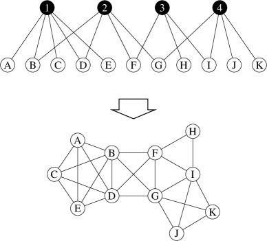
FIG. 14.: A schematic representation of a bipartite graph, such as the graph of movies and the actors who have appeared in them. In this small graph we have four movies, labeled $1$ to $4$, and eleven actors, labeled $A$ to $K$, with edges joining each movie to the actors in its cast. The bottom figure shows the one-mode projection of the graph for the eleven actors. After Newman et al. 2000.

It is worth noting, however, that some of the real-world networks presented in Sect. II, for example the collaboration networks, can be more completely described by bipartite graphs (Newman, Strogatz and Watts 2000). In a bipartite graph there are two kinds of nodes, and edges connect only nodes of different kind. For example, the collaboration network of movie actors is in fact a projection of a bipartite actor-movie graph, in which the two types of nodes are the actors and movies, and an edge connects each movie with the actors playing in it (see Fig. 14). The same argument stands for the collaboration between scientists (where scientists and papers are the two types of nodes) and metabolic networks (where nodes can be the substrates or reactions). The generating function method can be generalized to bipartite graphs (see Newman, Strogatz and Watts 2000), and it results in a nonvanishing clustering coefficient inherent to the bipartite structure

$$C=\frac{1}{1+\frac{(\mu_{2}-\mu_{1})(\nu_{2}-\nu_{1})^{2}}{\mu_{1}\nu_{1}(2\nu_{1}-3\nu_{2}+\nu_{3})}},$$ (64)

where $\mu_{n}=\sum_{k}k^{n}P_{a}(k)$ and $\nu_{n}=\sum_{k}k^{n}P_{m}(k)$, and in the actor-movie framework, $P_{a}(k)$ represents the fraction of actors which appeared in $k$ movies, while $P_{m}(k)$ means the fraction of movies in which $k$ actors have appeared.

The prediction of Eq. (64) has been tested for several collaboration graphs (Newman, Strogatz, Watts 2000), and in some cases there is an excellent agreement, but in others it deviates by a factor of $2$ from the clustering coefficient of the real network. Consequently we can conclude that the order present in real networks is not due solely to the definition of the network, but to a yet unknown organizing principle.

VI SMALL-WORLD NETWORKS

In Sects. II and III.A we have seen (see Table I, Figs. 8 and 9) that real-world networks have a small-world character like random graphs, but they have unusually large clustering coefficients. Furthermore, as Fig. 9 demonstrates, the clustering coefficient appears to be independent of the network size. This latter property is characteristic to ordered lattices, whose clustering coefficient is size independent and depends only on the coordination number. For example, a one-dimensional lattice with periodic boundary conditions (i.e. a ring of nodes), in which each node is connected to the $K$ nodes closest to it (see Fig. 15), most of the immediate neighbors of any site are also neighbors of one another, i.e. the lattice is clustered. For such a lattice the clustering coefficient is

$$C=\frac{3(K-2)}{4(K-1)},$$ (65)

which converges to $3/4$ in the limit of large $K$. Such low-dimensional regular lattices, however, do not have short path lengths: for a $d$ dimensional hypercubic lattice the average node-node distance scales as $N^{1/d}$, which increases much faster with $N$ than the logarithmic increase observed for random and real graphs. The first successful attempt to generate graphs with high clustering coefficients and small $\ell$ is due to Watts and Strogatz (1998).

A The Watts-Strogatz (WS) model

Watts and Strogatz (1998) proposed a one-parameter model which interpolates between an ordered finite dimensional lattice and a random graph. The algorithm behind the model is the following (Fig. 15):

(1) Start with order: Start with a ring lattice with $N$ nodes in which every node is connected to its first $K$ neighbors ($K/2$ on either side). In order to have a sparse but connected network at all times, consider $N\gg K\gg\ln(N)\gg 1$.

(2) Randomize: Randomly rewire each edge of the lattice with probability $p$ such that self-connections and duplicate edges are excluded. This process introduces $pNK/2$ long-range edges which connect nodes that otherwise would be part of different neighborhoods. Varying $p$ the transition between order ($p=0$) and randomness ($p=1$) can be closely monitored.

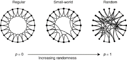
FIG. 15.: The random rewiring procedure of the WS model which interpolates between a regular ring lattice and a random network without altering the number of nodes or edges. We start with $N=20$ nodes, each connected to its $4$ nearest neighbors. For $p=0$ the original ring is unchanged; as $p$ increases the network becomes increasingly disordered until for $p=1$ all edges are rewired randomly. After Watts and Strogatz (1998).

This model has its roots in social systems where most people are friends with their immediate neighbors - neighbors on the same street, colleagues, people that their friends introduce them to. On the other hand, everybody has one or two friends who are a long way away - people in other countries, old acquaintances, which are represented by the long-range edges obtained by rewiring in the WS model.

To understand the coexistence of small path length and clustering, we study the behavior of the clustering coefficient $C(p)$ and the average path length $\ell(p)$ as a function of the rewiring probability $p$. For a ring lattice $\ell(0)\simeq N/2K\gg 1$ and $C(0)\simeq 3/4$, thus $\ell$ scales linearly with the system size, and the clustering coefficient is large. On the other hand, for $p\rightarrow 1$ the model converges to a random graph for which $\ell(1)\sim\ln(N)/\ln(K)$ and $C(1)\sim K/N$, thus $\ell$ scales logarithmically with $N$ and the clustering coefficient decreases with $N$. These limiting cases might suggest that large $C$ is always associated with large $\ell$, and small $C$ with small $\ell$. On the contrary, Watts and Strogatz (1998) found that there is a broad interval of $p$ over which $\ell(p)$ is close to $\ell(1)$ yet $C(p)\gg C(1)$ (Fig. 16). This regime originates in a rapid drop of $\ell(p)$ for small $p$ values, while $C(p)$ stays almost unchanged, resulting in networks that are clustered but have a small characteristic path length. This coexistence of small $\ell$ and large $C$ is in excellent agreement with the characteristics of real networks discussed in Sect. II, prompting many to call such systems small world networks.

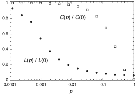
FIG. 16.: Characteristic path length $\ell(p)$ and clustering coefficient $C(p)$ for the WS model. The data is normalized by the values $\ell(0)$ and $C(0)$ for a regular lattice. A logarithmic horizontal scale resolves the rapid drop in $\ell(p)$, corresponding to the onset of the small-world phenomenon. During this drop $C(p)$ remains almost constant, indicating that the transition to a small world is almost undetectable at the local level. After Watts and Strogatz (1998).

B Properties of small-world networks

The pioneering article of Watts and Strogatz started an avalanche of research on the properties of small-world networks and the Watts-Strogatz (WS) model. A much studied variant of the WS model was proposed by Newman and Watts (1999a, 1999b) in which edges are added between randomly chosen pairs of sites, but no edges are removed from the regular lattice. This model is somewhat easier to analyze than the original Watts-Strogatz model because it does not lead to the formation of isolated clusters, whereas this can happen in the original model. For sufficiently small $p$ and large $N$ this model is equivalent with the WS model. In the following we will summarize the main results regarding the properties of small-world models.

1 Average path length

As we discussed above, in the WS model there is a change in the scaling of the characteristic path length $\ell$ as the fraction $p$ of the rewired edges is increased. For small $p$, $\ell$ scales linearly with the system size, while for large $p$ the scaling is logarithmic. As discussed by Watts (1999), and Pandit and Amritkar (1999), the origin of the rapid drop in $\ell$ is the appearance of shortcuts between nodes. Every shortcut, created at random, is likely to connect widely separated parts of the graph, and thus has a significant impact on the characteristic path length of the entire graph. Even a relatively low fraction of shortcuts is sufficient to drastically decrease the average path length, yet locally the network remains highly ordered.

An important question regarding the average path length is whether the onset of small-world behavior is dependent on the system size. It was Watts (1999) who first noticed that $\ell$ does not begin to decrease until $p\geq 2/NK$, guaranteeing the existence of at least one shortcut. This implies that the transition $p$ depends on the system size, or conversely, there exists a $p$-dependent crossover length $N^{*}$ such that if $N<N^{*}$, $\ell\sim N$, but if $N>N^{*}$, $\ell\sim\ln(N)$. The concept of the crossover length was introduced by Barthélémy and Amaral (1999a), who conjectured that the characteristic path length scales as (see Fig. 17):

$$\ell(N,p)\sim N^{*}F\left(\frac{N}{N^{*}}\right),$$ (66)

where

$$F(u)=\left\{\begin{array}[]{lcl}u&\mbox{if}&u\ll 1\\ \ln(u)&\mbox{if}&u\gg 1\end{array}\right..$$ (67)

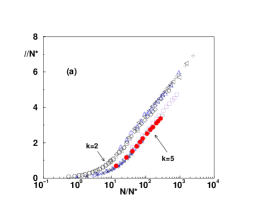
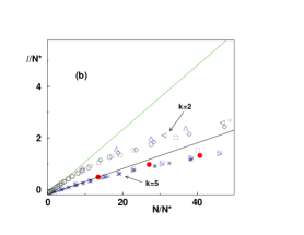
FIG. 17.: Data collapse $\ell(N,p)/N^{*}(p)$ versus $N/N^{*}(p)$ for two different values of $K$. (a) Log-linear scale showing the logarithmic behavior at large $N/N^{*}$; (b) Linear scale showing the linear behavior $\l(N,p)\sim N/(4K)$ at small $N/N^{*}$. After Barrat and Weigt (2000).

Numerical simulations and analytical arguments (Barthélémy and Amaral 1999a, Barrat 1999, Newman and Watts 1999a, Bartélémy and Amaral 1999b, Argollo de Menezes et al. 2000, Barrat and Weigt 2000) concluded that the crossover length $N^{*}$ scales with $p$ as $N^{*}\sim p^{-\tau}$ , where $\tau=1/d$ and $d$ is the dimension of the original lattice to which the random edges are added (Fig. 18). Thus for the original WS model, defined on a circle ($d=1$), we have $\tau=1$, the onset of small-world behavior taking place at the rewiring probability $p^{*}\sim 1/N$.

FIG. 18.: The dependence of the crossover length $N^{*}$ on the rewiring probability in one to four dimensions. The dashed lines represent the scaling relation $N^{*}\sim p^{-1/d}$. After Argollo de Menezes et al. (2000).

It is now widely accepted that the characteristic path length obeys the general scaling form

$$\ell(N,p)\sim\frac{N}{K}f(pKN^{d}),$$ (68)

where $f(u)$ is a universal scaling function that obeys

$$f(u)=\left\{\begin{array}[]{lcl}\mbox{constant}&\mbox{if}&u\ll 1\\ \ln(u)/u&\mbox{if}&u\gg 1\end{array}\right..$$ (69)

Newman et al. (1999) have calculated the form of the scaling function $f(u)$ for the one-dimensional small-world model using a mean-field method which is exact for small or large values of $u$, but not in the regime where $u\simeq 1$, obtaining

$$f(u)=\frac{4}{\sqrt{u^{2}+4u}}\tanh^{-1}\frac{u}{{\sqrt{u^{2}+4u}}}.$$ (70)

They also solved for the complete distribution of path lengths within this mean-field approximation.

The scaling relation (68) has been confirmed by extensive numerical simulations (Newman and Watts 1999a, Argollo de Menezes et al. 2000), renormalization group techniques (Newman and Watts 1999a) and series expansions (Newman and Watts 1999b). Equation (68) tells us that although the average path length in a small-world model appears at first glance to depend on three parameters - $p$, $K$ and $N$ - it is in fact entirely determined by a single scalar function $f(u)$ of a single scalar variable. Note that both the scaling function $f(u)$ and the scaling variable $u=pKN^{d}$ have simple physical interpretations. The variable $u$ is two times the average number of random links (shortcuts) on the graph for a given $p$, and $f(u)$ is the average of the fraction by which the distance between two nodes is reduced for a given $u$.

Several attempts have been made to calculate exactly the distribution of path lengths and the average path length $\ell$. Dorogovtsev and Mendes 2000a studied a simpler model which contains a ring lattice with directed edges of length $1$ and a central node which is connected with probability $p$ to the nodes of the lattice by undirected edges of length $0.5$. They calculated exactly the distribution of path lengths for this model, showing that $\ell/N$ depends only on the scaling variable $pN$ and the functional form of this dependence is similar to the numerically obtained $\ell(p)$ in the WS model. Kulkarni et al. 1999 calculated the probability $P(m|n)$ that two nodes separated by an Euclidian distance $n$ have a path length $m$. They have shown that the average path length $\ell$ is simply related to the mean $\langle s\rangle$ and the mean square $\langle s^{2}\rangle$ of the shortest distance between two diametrically opposite nodes (i.e. separated by the largest Euclidian distance), according to

$$\frac{\ell}{N}=\frac{\langle s\rangle}{N-1}-\frac{\langle s^{2}\rangle}{L(N-1)}.$$ (71)

Unfortunately calculating the shortest distance between opposite nodes is just as difficult as determining $\ell$ directly.

2 Clustering coefficient

In addition to a short average path length, small-world networks have a relatively high clustering coefficient. The WS model displays this duality for a wide range of the rewiring probabilities $p$. In a regular lattice ($p=0$) the clustering coefficient does not depend on the size of the lattice but only its topology. As the edges of the network are randomized, the clustering coefficient remains close to $C(0)$ up to relatively large values of $p$.

The dependence of $C(p)$ on $p$ can be derived using a slightly different but equivalent definition of $C$, introduced by Barrat and Weigt (2000). According to this definition, $C^{\prime}(p)$ is the fraction between the mean number of edges between the neighbors of a node and the mean number of possible edges between those neighbors. In a more graphic formulation (Newman, Strogatz and Watts 2000),

$$C^{\prime}=\frac{3\times\mbox{number of triangles}}{\mbox{number of connected triples}}.$$ (72)

Here triangles are trios of nodes in which each node is connected to both of the others, and connected triples are trios in which at least one is connected to both others, the factor $3$ accounting to the fact that each triangle contributes to $3$ connected triples. This definition corresponds to the concept of ”fraction of transitive triples” used in sociology (see Wasserman and Faust 1994).

To calculate $C^{\prime}(p)$ for the WS model, let us start with a regular lattice with a clustering coefficient $C(0)$. For $p>0$ two neighbors of a node $i$ that were connected at $p=0$ are still neighbors of $i$ and connected by and edge with probability $(1-p)^{3}$, since there are three edges which need to remain intact. Consequently $C^{\prime}(p)\simeq C(0)(1-p)^{3}.$ Barrat and Weigt (2000) have verified that the deviation of $C(p)$ from this expression is small and goes to zero as $N\rightarrow\infty$. The corresponding expression for the Newman-Watts model is (Newman, 2001e)

$$C^{\prime}(p)=\frac{3K(K-1)}{2K(2K-1)+8pK^{2}+4p^{2}K^{2}}.$$ (73)

3 Degree distribution

In the WS model for $p=0$ each node has the same degree $K$, thus the degree distribution is a delta function centered at $K$. A nonzero $p$ introduces disorder in the network, broadening the degree distribution while maintaining the average degree equal to $K$. Since only a single end of every edge is rewired ($pNK/2$ edges in total), each node has at least $K/2$ edges after the rewiring process. Consequently for $K>2$ there are no isolated nodes and the network is usually connected, unlike a random graph which consists of isolated clusters for a wide range of connection probabilities.

For $p>0$ the degree $k_{i}$ of a vertex $i$ can be written as (Barrat and Weigt 2000) $k_{i}=K/2+c_{i}$ where $c_{i}$ can be divided in two parts: $c_{i}^{1}\leq K/2$ edges have been left in place (with probability $1-p$), while $c_{i}^{2}=c_{i}-c_{i}^{1}$ edges have been rewired towards $i$, each with probability $1/N$. The probability distributions of $c_{i}^{1}$ and $c_{i}^{2}$ are

$$P_{1}(c_{i}^{1})=C_{K/2}^{c_{i}^{1}}(1-p)^{c_{i}^{1}}p^{K/2-c_{i}^{1}}$$ (74)

and

$$P_{2}(c_{i}^{2}) = C_{pNK/2}^{c_{i}^{2}}\left(\frac{1}{N}\right)^{c_{i}^{2}}\left(1-\frac{1}{N}\right)^{pNK/2-c_{i}^{2}}$$ (75)

$$\simeq \frac{(pK/2)^{c_{i}^{2}}}{c_{i}^{2}!}e^{-pK/2}$$ (76)

for large $N$. Combining these two factors together the degree distribution follows

$$P(k)=\sum_{n=0}^{f(k,K)}C_{K/2}^{n}(1-p)^{n}p^{K/2-n}\frac{(pK/2)^{k-K/2-n}}{(k-K/2-n)!}e^{-pK/2}$$ (77)

for $k\geq K/2$, where $f(k,K)=min(k-K/2,K/2)$.

FIG. 19.: Degree distribution of the WS model for $K=3$ and various $p$. We can see that only $k\geq K/2$ values are present, and the mean degree is $\langle k\rangle=K$. The symbols are obtained from numerical simulations of the WS model with $N=1000$, and the lines correspond to Eq. (77). As a comparison, the degree distribution of a random graph with the same parameters is plotted with filled symbols. After Barrat and Weigt (2000).

The shape of the degree distribution is similar to that of a random graph: it has a pronounced peak at $\langle k\rangle=K$ and decays exponentially for large $k$ (Fig. 19). Thus the topology of the network is relatively homogeneous, all nodes having approximately the same number of edges.

4 Spectral properties

As discussed in Sect. III.G, the spectral density $\rho(\lambda)$ of a graph reveals important information about its topology. Specifically, we have seen that for large random graphs $\rho(\lambda)$ converges to a semi-circle. It comes as no surprise that the spectrum of the WS model depends on the rewiring probability $p$ (Farkas et al. 2001). For $p=0$ the network is regular and periodical, consequently $\rho(\lambda)$ contains numerous singularities (Fig. 20a). For intermediate values of $p$ these singularities become blurred, but $\rho(\lambda)$ retains a strong skewness (Fig. 20b,c). Finally, as $p\rightarrow 1$, $\rho(\lambda)$ approaches the semi-circle law characterizing random graphs (Fig. 20d). While the details of the spectral density change considerably with $p$, the third moment of $\rho(\lambda)$ is consistently high, indicating a high number of triangles in the network. Thus the results summarized in Fig. 20 allow us to conclude that the high number of triangles is a basic property of the WS model (see also Gleis et al. 2000). The high regularity of small-world models for a broad range of $p$ is underlined by the results concerning the spectral properties of the Laplacian operator, which tells us about the time evolution of a diffusive field on the graph (Monasson 2000).

FIG. 20.: Spectral density of small-world networks, compared to the semi-circle law corresponding to random graphs (solid line). The rewiring probabilities are $p=0$ (a), $p=0.01$ (b), $p=0.3$ (c) and $p=1$ (d). After Farkas et al. (2001)

VII THE SCALE-FREE MODEL

The empirical results discussed in Sect. II demonstrate that many large networks are scale-free, that is, their degree distribution follows a power-law for large $k$. Furthermore, even for those networks for which $P(k)$ has an exponential tail, the degree distribution significantly deviates from a Poisson. We have seen in Sects. III.D and VI.B.3 that random graph theory and the WS model cannot reproduce this feature. While it is straightforward to construct random graphs which have power-law degree distribution (Sect. V), these constructions only postpone an important question: what is the mechanism responsible for the emergence of scale-free networks? We will see in this section that this quest will require a shift from modeling network topology to modeling the network assembly and evolution. While at this point these two approaches do not appear to be particularly distinct, we will find that there is a fundamental difference between the modeling approach we took in random graphs and the small-world models, and the one required to reproduce the power-law degree distribution. While the goal of the former models is to construct a graph with correct topological features, modeling scale-free networks will put the emphasis on capturing the network dynamics. That is, the underlying assumption behind evolving or dynamic networks is that if we capture correctly the processes that assembled the networks that we see today, then we will obtain their topology correctly as well. Dynamics takes the driving role, topology being only a byproduct of this modeling philosophy.

A Definition of the scale-free (SF) model

The origin of the power-law degree distribution in networks was first addressed by Barabási and Albert (1999), who argued that the scale-free nature of real networks is rooted in two generic mechanisms common in many real networks. The network models discussed thus far assume that we start with a fixed number $N$ of vertices that are then randomly connected or rewired, without modifying $N$. In contrast, most real world networks describe open systems which grow by the continuous addition of new nodes. Starting from a small nucleus of nodes, the number of nodes increases throughout the lifetime of the network by the subsequent addition of new nodes. For example the WWW grows exponentially in time by the addition of new web pages or the research literature constantly grows by the publication of new papers.

Second, network models discussed so far assume that the probability that two nodes are connected (or their connection is rewired) is independent of the nodes’ degree, i.e. new edges are placed randomly. Most real networks, however, exhibit preferential attachment, such that the likelihood of connecting to a node depends on the node’s degree. For example, a webpage will more likely include hyperlinks to popular documents with already high degree, because such highly connected documents are easy to find and thus well known, or a new manuscript is more likely to cite a well known and thus much cited publications than less cited and consequently less known papers.

These two ingredients, growth and preferential attachment, inspired the introduction of the scale-free (SF) model that has a power-law degree distribution. The algorithm of the SF model is the following:

(1) Growth: Starting with a small number ($m_{0}$) of nodes, at every timestep we add a new node with $m$($\leq m_{0}$) edges that link the new node to $m$ different nodes already present in the system.

(2) Preferential attachment: When choosing the nodes to which the new node connects, we assume that the probability $\Pi$ that a new node will be connected to node $i$ depends on the degree $k_{i}$ of node $i$, such that

$$\Pi(k_{i})=\frac{k_{i}}{\sum_{j}k_{j}}.$$ (78)

After $t$ timesteps this algorithm results in a network with $N=t+m_{0}$ nodes and $mt$ edges. Numerical simulations indicated that this network evolves into a scale-invariant state with the probability that a node has $k$ edges following a power-law with an exponent $\gamma_{SF}=3$ (see Fig. 21). The scaling exponent is independent of $m$, the only parameter in the model.

B Theoretical approaches

The dynamical properties of the scale-free model can be addressed using various analytic approaches. The continuum theory proposed by Barabási and Albert (1999), focuses on the dynamics of node degrees, followed by the master equation approach of Dorogovtsev, Mendes and Samukhin (2000a) and the rate equation approach introduced by Krapivsky, Redner and Leyvraz (2000). As these methods are often used interchangeably in the subsequent section, we review each of them next.

Continuum theory: The continuum approach introduced in Barabási and Albert (1999) and Barabási, Albert and Jeong (1999) calculates the time dependence of the degree $k_{i}$ of a given node $i$. This degree will increase every time a new node enters the system and links to node $i$, the probability of this process being $\Pi(k_{i})$. Assuming that $k_{i}$ is a continuous real variable, the rate at which $k_{i}$ changes is expected to be proportional to $\Pi(k_{i})$. Consequently, $k_{i}$ satisfies the dynamical equation

$$\frac{\partial k_{i}}{\partial t}=m\Pi(k_{i})=m\frac{k_{i}}{\sum_{j=1}^{N-1}k_{j}}.$$ (79)

The sum in the denominator goes over all nodes in the system except the newly introduced one, thus its value is $\sum_{j}k_{j}=2mt-m$, leading to

$$\frac{\partial k_{i}}{\partial t}=\frac{k_{i}}{2t}.$$ (80)

The solution of this equation, with the initial condition that every node $i$ at its introduction has $k_{i}(t_{i})=m$, is

$$k_{i}(t)=m\left(\frac{t}{t_{i}}\right)^{\beta},\quad\quad\mbox{with}\quad\beta=\frac{1}{2}.$$ (81)

Equation (81) indicates that the degree of all nodes evolves the same way, following a power-law, the only difference being the intercept of the power-law.

Using (81), the probability that a node has a degree $k_{i}(t)$ smaller than $k$, $P(k_{i}(t)<k)$, can be written as

$$P(k_{i}(t)<k)=P(t_{i}>{{m^{1/\beta}t}\over{k^{1/\beta}}}).$$ (82)

Assuming that we add the nodes at equal time intervals to the network, the $t_{i}$ values have a constant probability density

$$P(t_{i})=\frac{1}{m_{0}+t}.$$ (83)

Substituting this into Eq. (82) we obtain that

$$P\left(t_{i}>{{m^{1/\beta}t}\over{k^{1/\beta}}}\right)=1-{{m^{1/\beta}t}\over{k^{1/\beta}(t+m_{0})}}.$$ (84)

The degree distribution $P(k)$ can be obtained using

$$P(k)=\frac{\partial P(k_{i}(t)<k)}{\partial k}=\frac{2m^{1/\beta}t}{m_{0}+t}\,\frac{1}{k^{1/\beta+1}},$$ (85)

predicting that asymptotically ($t\rightarrow\infty$)

$$P(k)\sim 2m^{1/\beta}k^{-\gamma},\quad\mbox{with}\quad\gamma=\frac{1}{\beta}+1=3$$ (86)

being independent of $m$, in agreement with the numerical results.

FIG. 21.: (a) Degree distribution of the scale-free model, with $N=m_{0}+t=300,000$ and $m_{0}=m=1$ (circles), $m_{0}=m=3$ (squares), $m_{0}=m=5$ (diamonds) and $m_{0}=m=7$ (triangles). The slope of the dashed line is $\gamma=2.9$. The inset shows the rescaled distribution (see text) $P(k)/2m^{2}$ for the same values of $m$, the slope of the dashed line being $\gamma=3$. (b) $P(k)$ for $m_{0}=m=5$ and system sizes $N=100,000$ (circles), $N=150,000$ (squares) and $N=200,000$ (diamonds). The inset shows the time-evolution for the degree of two vertices, added to the system at $t_{1}=5$ and $t_{2}=95$. Here $m_{0}=m=5$, and the dashed line has slope $0.5$, as predicted by Eq. (81). After Barabási, Albert, Jeong (1999).

As the power-law observed for real networks describes systems of rather different sizes, it is expected that a correct model should provide a time-independent degree distribution. Indeed, Eq. (85) predicts that asymptotically the degree distribution of the SF model is independent of time (and, subsequently, independent of the system size $N=m_{0}+t$), indicating that despite its continuous growth, the network reaches a stationary scale-free state. Furthermore, Eq. (85) also indicates that the coefficient of the power-law distribution is proportional to $m^{2}$. All these predictions are confirmed by numerical simulations (see Fig. 21).

Master equation approach: The method introduced by Dorogovtsev, Mendes and Samukhin (2000a, see also Kullmann and Kertész 2000) studies the probability $p(k,t_{i},t)$ that at time $t$ a node $i$ introduced at time $t_{i}$ has a degree $k$. In the SF model when a new node with $m$ edges enters the system, the degree of node $i$ increases with $1$ with a probability $m\Pi(k)=k/2t$, otherwise it stays the same. Consequently the master equation governing $p(k,t_{i},t)$ for the SF model has the form

$$p(k,t_{i},t+1)=\frac{k-1}{2t}p(k-1,t_{i},t)+\left(1-\frac{k}{2t}\right)p(k,t_{i},t).$$ (87)

The degree distribution can be obtained as

$$P(k)=\lim_{t\rightarrow\infty}\left(\sum_{t_{i}}p(k,t_{i},t)\right)/t.$$ (88)

Eq. (87) implies that $P(k)$ is the solution of the recursive equation

$$P(k)=\left\{\begin{array}[]{lcl}\frac{k-1}{k+2}P(k-1)&\mbox{for}&k\geq m+1\\ 2/(m+2)&\mbox{for}&k=m\\ \end{array}\right..$$ (89)

giving

$$P(k)=\frac{2m(m+1)}{k(k+1)(k+2)},$$ (90)

very close to (86) obtained using the continuum theory.

Rate equation approach: The rate equation approach, introduced by Krapivsky, Redner and Leyvraz (2000), focuses on the average number $N_{k}(t)$ of nodes with $k$ edges at time $t$. When a new node enters the network in the scale-free model, $N_{k}(t)$ changes as

$$\frac{dN_{k}}{dt}=m\frac{(k-1)N_{k-1}(t)-kN_{k}(t)}{\sum_{k}kN_{k}(t)}+\delta_{k,m}.$$ (91)

Here the first term accounts for the new edges that connect to nodes with $k-1$ edges, thus increasing their degree to $k$. The second term describes the new edges connecting to nodes with $k$ edges turning them into nodes with $k+1$ edges, decreasing the number of nodes with $k$ edges. The third term accounts for the new nodes with $m$ edges. In the asymptotic limit $N_{k}(t)=tP(k)$ and $\sum_{k}kN_{k}(t)=2mt$, leading to the same recursive equation, (89), as predicted by the master equation approach.

The master equation and rate equation approaches are completely equivalent, and offer the same asymptotic results as the continuum theory. Thus for calculating the scaling behavior of the degree distribution they can be used interchangeably. In addition, these methods, not using a continuum assumption, appear more suitable to obtain exact results in more challenging network models.

C Limiting cases of the SF model

The the power-law scaling in the SF model indicates that growth and preferential attachment play an important role in network development. But are both of them necessary for the emergence of power-law scaling? To address this question, two limiting cases of the SF model have been investigated, which contain only one of these two mechanisms (Barabási and Albert 1999, Barabási, Albert and Jeong 1999).

Model A keeps the growing character of the network without preferential attachment. Starting with a small number of nodes ($m_{0}$), at every time step we add a new node with $m(\leq m_{0})$ edges. We assume that the new node connects with equal probability to the nodes already present in the system, i.e. $\Pi(k_{i})=1/(m_{0}+t-1)$, independent of $k_{i}$.

The continuum theory predicts that $k_{i}(t)$ follows a logarithmic time dependence, and for $t\rightarrow\infty$ the degree distribution decays exponentially, following (Fig. 22a)

$$P(k)=\frac{e}{m}\exp\left(-\frac{k}{m}\right).$$ (92)

The exponential character of the distribution indicates that the absence of preferential attachment eliminates the scale-free character of the resulting network.

Model B starts with $N$ nodes and no edges. At each time step a node is selected randomly and connected with probability $\Pi(k_{i})=k_{i}/\sum_{j}k_{j}$ to a node $i$ in the system. Consequently, model B eliminates the growth process, the number of nodes being kept constant during the network evolution. Numerical simulations indicate that while at early times the model exhibits power-law scaling, $P(k)$ is not stationary (Fig 22). Since $N$ is constant, and the number of edges increases with time, after $T\simeq N^{2}$ timesteps the system reaches a state in which all nodes are connected.

The time-evolution of the individual degrees can be calculated analytically using the continuum theory, indicating that

$$k_{i}(t)\simeq\frac{2}{N}t,$$ (93)

assuming $N>>1$, in agreement with the numerical results ( Fig. 22b).

Since the continuum theory predicts that after a transient period the average degree of all nodes should have the same value given by Eq. (93), we expect that the degree distribution becomes a Gaussian around its mean value. Indeed, Fig. 22b shows that the shape of $P(k)$ changes from the initial power-law to a Gaussian.

Motivated by correlations between stocks in finantial markets and airline route maps, a prior model incorporating preferential attachment, while keeping $N$ constant was independently proposed and studied by Amaral et al. (1999).

FIG. 22.: (a) Degree distribution for model A for $m_{0}=m=1$ (circles), $m_{0}=m=3$ (squares), $m_{0}=m=5$ (diamonds) and $m_{0}=m=7$ (triangles). The size of the network is $N=800,000$. Inset: time evolution for the degree of two vertices added to the system at $t_{1}=7$ and $t_{2}=97$. Here $m_{0}=m=3$. The dashed line follows $k_{i}(t)=m\ln(m_{0}+t-1)$.(b) The degree distribution for model B for $N=10,000$ and $t=N$ (circles), $t=5N$ (squares), and $t=40N$ (diamonds). Inset: time dependence of the degrees of two vertices. The system size is $N=10,000$. After Barabási, Albert and Jeong (1999).

The failure of models A and B to lead to a scale-free distribution indicates that growth and preferential attachment are needed simultaneously to reproduce the stationary power-law distribution observed in real networks.

D Properties of the SF model

While the SF model captures the power-law tail of the degree distribution, it has other properties which may or may not agree with empirical results on real networks. As we discussed in Sect. I, a characteristic feature of real networks is the coexistence of clustering and short path lengths. Thus we need to investigate if the network generated by the SF model has a small-world character.

1 Average path length

Figure 23 shows the average path length of a network with average degree $\langle k\rangle=4$ generated by the SF model as a function of the network size, $N$, compared with the average path length of a random graph with the same size and average degree. The figure indicates that the average path length is smaller in the SF network than in a random graph for any $N$, indicating that the heterogeneous scale-free topology is more efficient in bringing the nodes close than the homogeneous topology of random graphs. We find that the average path length of the SF network increases approximately logarithmically with $N$, the best fit following a generalized logarithmic form

$$\ell=A\log(N-B)+C.$$ (94)

FIG. 23.: Characteristic path length $\ell$ versus network size $N$ in a network with $\langle k\rangle=4$ generated by the SF model (circles), compared with a random graph with the same size and average degree generated with the algorithm described in Sect. III.A (squares). The dashed line follows Eq. (94), and the solid lines represent Eq. [59] with $z_{1}=\langle k\rangle$ and $z_{2}$ the numerically obtained number of second neighbors in the respective networks.

In Figure 23 we also show the prediction of Eq. (59) for these networks, using the numerically determined number of first and second neighbors. While the fit is good for the random graph, Eq. (59) systematically underestimates the average path length of the SF network, as it does with the average path length of real networks (see Table II, last three columns).

In summary, apart from the empirical fit (94) there is no theoretical expression that would give a good approximation for the path length in the scale-free model (although encouraging first steps concerning the loop structure were made in Gleis et al. 2000). The failure of (59) underlies the fact that the topology of the network generated by the SF model is different from the topology of a random network with power-law degree distribution (Sect. V). The dynamical process that generates the network introduces nontrivial correlations that affect all topological properties.

2 Node degree correlations

In the random graph models with arbitrary degree distribution (see Abello et al. 2000 and Newman et al. 2000) the node degrees are uncorrelated. Krapivsky and Redner (2000) have shown that in the SF model correlations develop spontaneously between the degree of connected nodes.

Let us consider all node pairs with degree $k$ and $l$ connected by an edge. Without loss of generality we assume that the node with degree $k$ was added later to the system, implying that $k<l$ since, according to Eq. (81), older nodes have higher degree than younger ones, and for simplicity we use $m=1$. Denoting by $N_{kl}(t)$ the number of connected pairs of nodes with degree $k$ and $l$, we have

$$\frac{dN_{kl}}{dt} = \frac{(k-1)N_{k-1,l}-kN_{kl}}{\sum_{k}kN(k)}+\frac{(l-1)N_{k,l-1}-lN_{kl}}{\sum_{k}kN(k)}$$ (95)

$$+ (l-1)N_{l-1}\delta_{k1}.$$ (96)

The first term on the r.h.s. accounts for the change in $N_{kl}$ due to the addition of an edge to a node of degree $k-1$ or $k$ which is connected to a node of degree $l$. Since the addition of a new edge increases the node’s degree by $1$, the first term in the numerator corresponds to a gain in $N_{kl}$, while the second to a loss. The second term on the r.h.s. incorporates the same effects as the first applied to the other node. The last term takes into account the possibility that $k=1$, thus the edge that is added to the node with degree $l-1$ is the same edge that connects the two nodes.

This equation can be transformed into a time-independent recursion relation using the hypotheses $\sum_{k}kN(k)\rightarrow 2t$ and $N_{kl}(t)\rightarrow tn_{kl}$. Solving for $n_{kl}$ we obtain

$$n_{kl} = \frac{4(l-1)}{k(k+1)(k+l)(k+l+1)(k+l+2)}$$ (97)

$$+ \frac{12(l-1)}{k(k+l-1)(k+l)(k+l+1)(k+l+2)}.$$ (98)

For a network with an arbitrary degree distribution, if the edges are placed randomly, $n_{kl}=n_{k}n_{l}$. The most important feature of the result (97) is that the joint distribution does not factorize, i.e. $n_{kl}\neq n_{k}n_{l}$. This indicates the spontaneous appearance of correlations between the degrees of the connected nodes. The only case when $n_{kl}$ can be simplified to a factorized expression is when $1\ll k\ll l$, and $n_{kl}$ becomes

$$n_{kl}\simeq k^{-2}l^{-2},$$ (99)

but even then it is different from $n_{kl}=k^{-3}l^{-3}$, expected if correlations are absent from the network. This result offers the first explicit proof that the dynamical process that creates the scale-free network builds up nontrivial correlations between the nodes that are not present in the uncorrelated models discussed in Sect.V.

3 Clustering coefficient

While the clustering coefficient has been much investigated for the WS model (Sect. VI.B.2), there is no analytical prediction for the SF model. Figure 24 shows the clustering coefficient of the SF network with average degree $\langle k\rangle=4$ and different sizes, compared with the clustering coefficient $C_{rand}=\langle k\rangle/N$ of a random graph. We find that the clustering coefficient of the scale-free network is about $5$ times higher than that of the random graph, and this factor slowly increases with the number of nodes. However, the clustering coefficient of the SF model decreases with the network size following approximately a power-law $C\sim N^{-0.75}$, which, while a slower decay than the $C=\langle k\rangle N^{-1}$ decay observed for random graphs, is still different from the behavior of the small-world models, where $C$ is independent of $N$.

FIG. 24.: Clustering coefficient versus size of the SF model with $\langle k\rangle=4$, compared with the clustering coefficient of a random graph, $C_{rand}\simeq\langle k\rangle/N$.

4 Spectral properties

The spectral density of the scale-free model is continuous, but it has a markedly different shape than the semicircular spectral density of random graphs (Farkas et al. 2001, Goh, Kahng and Kim 2001). Numerical simulations indicate that the bulk of $\rho(\lambda)$ has a triangle-like shape with top lying well above the semi-circle and edges decaying as a power-law (Fig. 25). This power-law decay is due to the eigenvectors localized on the highest degree nodes. As in the case of random graphs (and unlike small-world networks), the principal eigenvalue, $\lambda_{1}$, is clearly separated from the bulk of the spectrum. A lower bound for $\lambda_{1}$ can be given as the square-root of the network’s largest degree $k_{1}$, and since the node degrees in the scale-free model increase as $N^{1/2}$, it results that $\lambda_{1}$ increases approximately as $N^{1/4}$. Numerical results indicate that $\lambda_{1}$ deviates from the expected behavior for small network sizes, reaching it asymptotically for $N\rightarrow\infty$. This crossover indicates the presence of correlations between the longest row vectors, offering additional evidence for correlations in the scale-free model.

FIG. 25.: Rescaled spectral density of three networks generated by the scale-free model having $m=m_{0}=5$ and size $N=100$ (continuous line), $N=300$ (dashed line) and $N=1000$ (short-dashed line). The semi-circle law corresponding to random graphs is drawn for comparison. The isolated peak corresponds to the largest eigenvalue, which increases as $N^{1/4}$. Inset: the edge of the spectral density decays as a power-law. After Farkas et al. (2001).

The principal eigenvalue plays an important role in the moments of $\rho(\lambda)$, determining the loop structure of the scale-free network. In contrast with the subcritical random graph (i.e. $p<1/N$), where the fraction of loops becomes negligible, in a scale-free network the fraction of loops with more than four edges increases with $N$, and their growth rate increases with the size of the loop. Note that the fraction of triangles decreases as $N\rightarrow\infty$ (Gleis et al. 2000, Bianconi 2000b).

While for random graphs $\rho(\lambda)$ follows the semi-circle law (Wigner 1955, 1957, 1958), deriving a similarly simple expression for small-world (see Sect. VI.B.4) and scale-free networks remains a considerable challenge.

VIII EVOLVING NETWORKS

The scale-free model discussed in the previous section is a minimal model that captures the mechanisms responsible for the power-law degree distribution. Compared to real networks, it is easy to notice its limitations: it predicts a power-law degree distribution with a fixed exponent, while the exponents measured for real networks vary between $1$ and $3$ (see Table II). Also, the degree distribution of real networks can have non-power-law features like exponential cutoffs (see Amaral et al. 2000, Newman 2001b,c and Jeong et al. 2001) or a saturation for small $k$. The discrepancies between the model and real networks led to a surge of research aiming to answer several basic questions of network evolution: How can we change the scaling exponents? Are there universality classes similar to those seen in critical phenomena, characterized by unique exponents? How do various microscopic processes, known to be present in real networks, influence the network topology? Are there quantities, beyond the degree distribution, that could help classifying networks? While the community is still in the process of answering these questions, several robust results are already available, offering much insight into network evolution and topology.

A Preferential attachment $\Pi(k)$

A central ingredient of all models aiming to generate scale-free networks is preferential attachment, i.e. the assumption that the likelihood of receiving new edges increases with the node’s degree. The SF model assumes that the probability $\Pi(k)$ that a node attaches to node $i$ is proportional to the degree $k$ of node $i$ (see Eq. (78)). This assumption involves two hypotheses: the first that $\Pi(k)$ depends on $k$, in contrast with random graphs in which $\Pi(k)=p$. Second, the functional form of $\Pi(k)$ is linear in $k$. The precise form of $\Pi(k)$ is more than a purely academic question, as lately a series of studies have demonstrated that the degree distribution depends strongly on $\Pi(k)$. To review these developments we start by discussing the empirical results on the functional form of $\Pi(k)$, followed by the theoretical work predicting the effect of $\Pi(k)$ on the network topology.

1 Measuring $\Pi(k)$ for real networks

The functional form of $\Pi(k)$ can be determined for networks for which we know the time at which each node joined the network (Jeong, Néda, Barabási 2001, Newman 2001d, Pastor-Satorras et al. 2001). Such dynamical data is available for the coauthorship network of researchers, the citation network of articles, the actor collaboration network and the Internet at the domain level (see Sect. II).

Consider the state of the network at a given time, and record the number of ”old” nodes present in the network and their degrees. Next measure the increase of the degree of the ”old” nodes over a time interval $\Delta T$, much shorter than the age of the network. Then, according to (78), plotting the relative increase $\Delta k_{i}/\Delta k$ in function of the earlier degree $k_{i}$ for every node gives the $\Pi(k)$ function. Here $\Delta k$ is the number of edges added to the network in the time $\Delta T$. We can reduce the fluctuations in the data by plotting the cumulative distribution

$$\kappa(k)=\sum_{k_{i}=0}^{k}\Pi(k_{i}).$$ (100)

FIG. 26.: Cumulated preferential attachment for (a) the citation network; (b) the Internet; (c) the neuroscience scientific collaboration network; (d) the actor collaboration network. In all panels the dashed line corresponds to linear preferential attachment, and the continuous line to no preferential attachment. After Jeong, Néda, Barabási (2001).

As Fig. 26 shows, the obtained $\Pi(k)$ supports the existence of preferential attachment. Furthermore, it appears that in each case $\Pi(k)$ follows a power-law, i.e.

$$\Pi(k)\sim k^{\alpha}.$$ (101)

While in some cases, such as the Internet (Jeong, Néda, Barabási 2001, Pastor-Satorras et al. 2001), citation network (Jeong, Néda , Barabási 2001), Medline and Los Alamos archive (Newman 2001d) we have $\alpha\simeq 1$, i.e. $\Pi(k)$ depends linearly on $k$ as assumed in the SF model, for some collaboration networks the dependence is sublinear, having $\alpha=0.8\pm 0.1$ for the neuroscience coauthorship and the actor collaboration network (Jeong et al. 2001).

2 Nonlinear preferential attachment

The effect of a nonlinear $\Pi(k)$ on the network dynamics and topology was explained by Krapivsky, Redner and Leyvraz (2000). Replacing the linear preferential attachment (78) with (101) in a directed network model, Krapivsky, Redner and Leyvraz calculate the average number $N_{k}(t)$ of nodes with $k-1$ incoming edges at time $t$ by the rate equation approach (see Sect. VII.B). The time evolution of $N_{k}(t)$ follows

$$\frac{dN_{k}}{dt}=\frac{1}{M_{\alpha}}[(k-1)^{\alpha}N_{k-1}-k^{\alpha}N_{k}]+\delta_{k1},$$ (102)

where $M_{\alpha}(t)=\sum k^{\alpha}N_{k}(t)$ is the $\alpha$th moment of $N_{k}(t)$. In (102) the first term accounts for the new nodes that connect to nodes with $k-1$ edges, thus increasing their degree to $k$. The second term describes the new nodes connecting to nodes with $k$ edges turning them into nodes with $k+1$ edges, decreasing the number of nodes with $k$ edges. The third term accounts for the continuous introduction of new nodes with a single outgoing edge.

Depending on the value of $\alpha$, several distinct phases have been identified:

Sub-linear case ($\alpha<1$): In this regime in the long-time limit $M_{\alpha}(t)$ satisfies $M_{\alpha}(t)=\mu t$, with a prefactor $1\leq\mu=\mu(\alpha)\leq 2$. Substituting $M_{\alpha}(t)$ and $N_{k}$ into Eq. (102) we obtain the degree distribution

$$P(k)=\frac{\mu}{k^{\alpha}}\prod_{j=1}^{k}\left(1+\frac{\mu}{j^{\alpha}}\right)^{-1}.$$ (103)

This product can be expanded in series, and the result is a stretch-exponential in which a new term arises whenever $\alpha$ decreases below $1/l$, where $l$ is an arbitrary positive integer.

Superlinear preferential attachment ($\alpha>1$): In this regime Eq. (102) has no analytical solution, but its discretized version can be used to determine recursively the leading behavior of each $N_{k}$ as $t\rightarrow\infty$. For $\alpha>2$ a ”winner-takes-all” phenomenon emerges, such that almost all nodes have a single edge, connecting them to a ”gel” node which has the rest of edges of the network. For $3/2<\alpha<2$ the number of nodes with two edges grows as $t^{2-\alpha}$, while the number of nodes with more than two edges is again finite. Again, the rest of the edges belong to the gel node. In general for $(l+1)/l<\alpha<l/(l-1)$ the number of nodes with more than $l$ edges is finite even in infinite systems, while $N_{k}\sim t^{k-(k-1)\alpha}$ for $k\leq l$.

In conclusion, the analytical calculations of Krapivsky, Redner and Leyvraz demonstrate that the scale-free nature of the network is destroyed for nonlinear preferential attachment. The only case in which the topology of the network is scale-free is when the preferential attachment is asymptotically linear, i.e. $\Pi(k_{i})\sim a_{\infty}k_{i}$ as $k_{i}\rightarrow\infty$. In this case the rate equation leads to

$$P(k)\sim k^{-\gamma}\quad\quad\mbox{with}\quad\gamma=1+\frac{\mu}{a_{\infty}}.$$ (104)

This way the exponent of the degree distribution can be tuned to any value between $2$ and $\infty$.

3 Initial attractiveness

Another general feature of $\Pi(k)$ in real networks is that $\Pi(0)\neq 0$, i.e. there is a nonzero probability that a new node attaches to an isolated node (Jeong, Néda, Barabási 2001). Thus in general $\Pi(k)$ has the form

$$\Pi(k)=A+k^{\alpha},$$ (105)

where $A$ is the initial attractiveness of the node $i$ (Dorogovtsev, Mendes, Samukhin 2000a). Indeed, if $A=0$, a node that has $k=0$ can never increase its connectivity according to Eq. (78). However, in real networks every node has a finite chance to be ”discovered” and linked to even if it has no edges to start with. Thus the parameter $A$ describes the likelihood that an isolated node is discovered, such as a new article is cited the first time.

Dorogovtsev, Mendes and Samukhin (2000a) gave an exact solution for a class of growing network models using the master equation approach (see Sect. VII.B). In their model at every timestep a new node is added to the network, followed by the addition of $m$ directed edges pointing from any node in the network to preferentially chosen nodes. The probability that a node receives an incoming edge is proportional to the sum of an initial attractiveness and the number of its incoming edges, i.e. $\Pi(k_{in})=A+k_{in}$. The calculations indicate that the degree distribution follows $P(k)\sim k^{-\gamma}$ with $\gamma=2+\frac{A}{m}$. Consequently, initial attractiveness does not destroy the scale-free nature of the degree distribution, only changes the degree exponent. These results agree with the conclusion of Krapivsky, Redner and Leyvraz (2000), who find that the power-law $P(k)$ is preserved for a shifted linear $\Pi(k)$, since the effect of the initial attractiveness diminishes as $k\rightarrow\infty$. A generalization of the Dorogovtsev, Mendes, Samukhin model (Dorogovtsev, Mendes and Samukhin 2000b) allows for the random distribution of $n_{r}$ edges and an initial degree $n$ of every new node. These changes do not modify the asymptotically linear scaling of the preferential attachment, thus this model also gives a power-law degree distribution with $\gamma=2+(n_{r}+n+A)/m$.

B Growth

In the SF model the number of nodes and edges increases linearly in time, and consequently the average degree of the network is constant. In this section we discuss the effect of the nonlinear growth rates on the network dynamics and topology.

1 Empirical results

The fact that networks can follow different growth patterns is supported by several recent measurements. For example, the average degree of the Internet in November of 1997 was $3.42$, but it increased to $3.96$ by December of 1998 (Faloutsos et al. 1999). Similarly, the WWW has increased its average degree from $7.22$ to $7.86$ in the five months between the measurements of Broder et al. (2000). The average degree of the coauthorship network of scientists has been found to continuously increase over an eight year period (Barabási et al. 2000). Finally, comparison of the metabolic network of organisms of different sizes indicates that the average degree of the substrates increases approximately linearly with the number of substrates involved in the metabolism (Jeong et al. 2000). The increase of the average degree indicates that in many real systems the number of edges increases faster than the number of nodes, supporting the presence of a phenomenon called accelerated growth.

2 Analytical results

Dorogovtsev and Mendes (2000d) studied analytically the effect of accelerated growth on the degree distribution, generalizing the directed model with asymptotically linear preferential attachment of Dorogovtsev, Mendes and Samukhin 2000a (Sect VIII.A). In this model at every step a new node is added to the network which receives $n$ incoming edges from random nodes in the system. Additionally $c_{0}t^{\theta}$ new edges are distributed, each of them being directed from a randomly selected node to a node with high incoming degree with asymptotically linear preferential attachment $\Pi(k_{in})\propto A+k_{in}$. The authors show that accelerated growth, controlled by the exponent $\theta$, does not change the scale-free nature of the degree distribution, but it modifies the degree exponent, which now becomes

$$\gamma=1+\frac{1}{1+\theta}.$$ (106)

While the model of Dorogovtsev and Mendes (2000d) is based on a directed network, Barabási et al. 2001 discuss an undirected model motivated by measurements on the evolution of the coauthorship network. In the model new nodes are added to the system with a constant rate, and these new nodes connect to $b$ nodes already in the system with preferential attachment

$$P_{i}=b\frac{k_{i}}{\sum_{j}k_{j}}.$$ (107)

Additionally, at every timestep a linearly increasing number of edges (constituting a fraction $a$ of the nodes which are present in the network) are distributed between the nodes, the probability that an edge is added between nodes $i$ and $j$ being

$$P_{ij}=\frac{k_{i}k_{j}}{\sum_{s,l}^{{}^{\prime}}k_{s}k_{l}}N(t)a.$$ (108)

Here $N(t)$ is the number of nodes in the system and the summation goes over all non-equal values of $s$ and $l$. As a result of these two processes the average degree of the network increases linearly in time, following $\langle k\rangle=at+2b$, in agreement with the measurements on the real coauthor network. The continuum theory predicts that the time-dependent degree distribution displays a crossover at a critical degree

$$k_{c}=\sqrt{b^{2}t}(2+2at/b)^{3/2},$$ (109)

such that for $k\ll k_{c}$, $P(k)$ follows a power-law with exponent $\gamma=1.5$ and for $k\gg k_{c}$ the exponent is $\gamma=3$. This result explains the fast-decaying tail of the degree distributions measured by Newman (2001a), and it indicates that as time increases the scaling behavior with $\gamma=1.5$ becomes increasingly visible. An equivalent model, proposed by Dorogovtsev and Mendes (2001), was able to reproduce the two separate power-law regimes in the distribution of word coocurences (Ferrer i Cancho, Solé 2001).

C Local events

The SF model incorporates only one mechanism for network growth: the addition of new nodes that connect to the nodes already in the system. In real systems, however, a series of microscopic events shape the network evolution, including the addition or rewiring of new edges or the removal of nodes or edges. Lately several models have been proposed to investigate the effect of selected processes on the scale-free nature of the degree distribution, offering a more realistic description of various real networks. Any local change in the network topology can be obtained through a combination of four elementary processes: addition and removal of a node and addition or removal of an edge. But in reality these events come jointly, such as the rewiring of an edge is a combination of an edge removal and addition. Next we briefly review several studies that address in general terms the effect of local events on the network topology.

1 Internal edges and rewiring

A model that incorporates new edges between existing nodes and the rewiring of edges was discussed by Albert and Barabási (2000). Starting with $m_{0}$ isolated nodes, at each timestep we perform one of the following three operations:

(i) With probability $p$ we add $m$($m\leq m_{0}$) new edges. One end of a new edge is selected randomly, the other with probability

$$\Pi(k_{i})=\frac{k_{i}+1}{\sum_{j}(k_{j}+1)}.$$ (110)

(ii) With probability $q$ we rewire $m$ edges. For this we randomly select a node $i$ and remove an edge $l_{ij}$ connected to it, replacing it with a new edge $l_{ij^{\prime}}$ that connects $i$ with node $j^{\prime}$ chosen with probability $\Pi(k_{j}^{\prime})$ given by (110).

(iii) With probability $1-p-q$ we add a new node. The new node has $m$ new edges that with probability $\Pi(k_{i})$ are connected to nodes $i$ already present in the system.

In the continuum theory the growth rate of the degree of a node $i$ is given by:

$$\frac{\partial k_{i}}{\partial t}=(p-q)m\frac{1}{N}+m\frac{k_{i}+1}{\sum_{j}(k_{j}+1)}.$$ (111)

The first term in the r.h.s. corresponds to the random selection of node $i$ as a starting point of a new edge (with probability $p$) or as the endpoint from which an edge is disconnected (with probability $q$). The second term corresponds to the selection of node $i$ as an endpoint of an edge with the preferential attachment present in all three of the possible processes.

The solution of (111) has the form

$$k_{i}(t)=\left(A(p,q,m)+m+1\right)\left(\frac{t}{t_{i}}\right)^{\frac{1}{B(p,q,m)}}-A(p,q,m)-1,$$ (112)

where

$$A(p,q,m) = (p-q)\left(\frac{2m(1-q)}{1-p-q}+1\right),$$ (113)

$$B(p,q,m) = \frac{2m(1-q)+1-p-q}{m}.$$ (114)

The corresponding degree distribution has the generalized power-law form

$$P(k)\propto(k+\kappa(p,q,m))^{-\gamma(p,q,m)},$$ (115)

where $\kappa(p,q,m)=A(p,q,m)+1$ and $\gamma(p,q,m)=B(p,q,m)+1$.

Eq. (115) is valid only when $A(p,q,m)+m+1>0$, which, for fixed $p$ and $m$, translates into $q<q_{max}={\rm min}\{1-p,(1-p+m)/(1+2m)\}$. Thus the $(p,q)$ phase diagram separates into two regions: For $q<q_{max}$ the degree distribution is given by (115), following a generalized power-law. For $q>q_{max}$, however, Eq.(115) is not valid, but numerical simulations indicate that $P(k)$ approaches an exponential.

While a power-law tail is present in any point of the scale-free regime, for small $k$ the probability saturates at $P(\kappa(p,q,m))$, a feature seen in many real networks (Fig 3b,d). Also, the exponent $\gamma(p,q,m)$ characterizing the tail of $P(k)$ for $k>>\kappa(p,q)$ changes continuously with $p$, $q$ and $m$, predicting a range of exponents between 2 and $\infty$. The realistic nature of $P(k)$ was confirmed by successfully fitting it to the degree distribution of the actor collaboration network (Albert and Barabási 2000).

2 Internal edges and edge removal

Dorogovtsev and Mendes (2000c) consider a class of undirected models in which new edges are added between old sites and existing edges can be removed. In the first variant of the model called developing network, $c$ new edges are introduced at every timestep, which connect two unconnected nodes $i$ and $j$ with a probability proportional to the product of their degrees (as in Eq. 108), an assumption confirmed by the empirical measurements on the coauthorship network (Barabási et al. 2000). It is assumed that $c$ can be tuned continuously, such that $c>0$ for the developing and $c<0$ for the decaying network. The continuum theory predicts that the rate of change of the node degrees has the form

$$\frac{\partial k_{i}}{\partial t}=\frac{k_{i}(t)}{\int_{0}^{t}k_{j}(t)dt_{j}}+2c\frac{k_{i}(t)\left[\int_{0}^{t}k_{j}(t)dt_{j}-k_{i}(t)\right]}{\left[\int_{0}^{t}k_{j}(t)dt_{j}\right]^{2}-\int_{0}^{t}k^{2}_{j}(t)dt_{j}},$$ (116)

where the summation over all nodes $\sum_{j}k_{j}$ has been approximated by an integral over all introduction times $t_{j}$. The first term in the right hand side incorporates linear preferential attachment, while the second term corresponds to the addition of $c$ new edges. Every node can be at either end of the new edge, and the probability of a node $i$ becoming an end of the new edge is proportional to the product of its degree $k_{i}$ and the sum of the degrees $k_{j}$ of all other nodes. The normalization factor is the sum of all products $k_{i}k_{j}$ with $i$ different from $j$.

In the asymptotic limit the second term can be neglected compared with the first term in both the numerator and denominator, and (116) becomes

$$\frac{\partial k_{i}}{\partial t}=(1+2c)\frac{k_{i}(t)}{\int_{0}^{t}k_{j}(t)dt_{j}},$$ (117)

which predicts the dynamic exponent (81) as

$$\beta=\frac{1+2c}{2(1+c)},$$ (118)

and the degree exponent as

$$\gamma=2+\frac{1}{1+2c}.$$ (119)

The limiting cases of this developing network are $c=0$ when the familiar SF values $\beta=1/2$ and $\gamma=3$ are obtained, and $c\rightarrow\infty$, when $\beta\rightarrow 1$ and $\gamma\rightarrow 2$.

In the decaying network at every timestep $|c|$ edges are removed randomly. The decrease of the node degrees due to this process is proportional to their current value, so equation (117) applies here as well, the only difference being that now $c<0$. A more rigorous calculation accounting for the fact that only existing edges can be removed confirms that the end result is identical with Eqs. (118) and (119), only with negative $c$. The limiting value of $c$ is $-1$, since the rate of removal of edges cannot be higher than the rate of addition of new nodes and edges, leading to the limit exponents $\beta\rightarrow-\infty$ and $\gamma\rightarrow\infty$.

D Growth constraints

For many real networks the nodes have a finite lifetime (for example in social networks) or a finite edge capacity (Internet routers or nodes in the electrical power grid). Recently several groups have addressed the degree to which such constraints effect the degree distribution.

1 Aging and cost

Amaral et al. (2000) suggested that while several networks do show deviations from the power-law behavior, they are far from being random networks. For example, the degree distribution of the electric powergrid of Southern California and of the neural network of the worm C. elegans is more consistent with a single-scale exponential distribution. Other networks, like the extended actor collaboration network, in which TV films and series are included, have a degree distribution in which the power-law scaling is followed by an exponential cutoff for large $k$. In all these examples there are constraints limiting the addition of new edges. For example, the actors have a finite active period during which they are able to collect new edges, while for the electrical powergrid or neural networks there are constraints on the total number of edges a particular node can have, driven by economic, physical or evolutionary reasons. Amaral et al. propose that in order to explain these deviations from a pure power-law we need to incorporate aging and cost or capacity constraints. The model studied by them evolves following growth and preferential attachment, but when a node reaches a certain age (aging) or has more than a critical number of edges (capacity constraints), new edges cannot connect to it. In both cases numerical simulations indicate that while for small $k$ the degree distribution still follows a power-law, for large $k$ an exponential cutoff develops (Fig. 27).

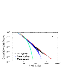
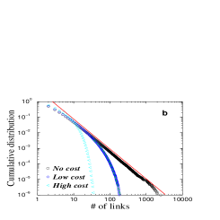
FIG. 27.: Deviation from a power-law of the degree distribution due to adding age (a) and capacity (b) constraints to the SF model. The constraints result in cutoffs of the power-law scaling. After Amaral et al. (2000).

FIG. 28.: The dependence of the degree exponent $\gamma$ on the aging exponent $\nu$ in the model of Dorogovtsev and Mendes (2000b). The points are obtained from simulations, while the solid line is the prediction of the continuum theory. After Dorogovtsev and Mendes (2000b).

2 Gradual aging

Dorogovtsev and Mendes (2000b) propose that in some systems the probability that a new node connects to a node $i$ is proportional not only to the degree $k_{i}$ of node $i$, but it also depends on its age, decaying as, $(t-t_{i})^{-\nu}$, where $\nu$ is a tunable parameter. Papers or actors gradually lose their ability to attract more edges, the model assuming that this phase-out follows a power-law. The calculations predict that the degree distribution depends on the exponent $\nu$: the power-law scaling is present only for $\nu<1$, and the degree exponent depends on $\nu$ (Fig. 28). Moreover, when $\nu>1$ the power-law scaling completely disappears, the degree distribution approaching an exponential.

E Competition in evolving networks

The SF model assumes that all nodes increase their degree following a power-law time dependence with the same dynamic exponent $\beta=1/2$ (Eq. (81)). As a consequence, the oldest nodes have the highest number of edges, since they had the longest lifetime to accumulate them. However, numerous examples indicate that in real networks a node’s degree and growth rate do not depend on age alone. For example, on the World-Wide Web some documents acquire a large number of edges in a very short time through a combination of good content and marketing (Adamic and Huberman 2000), or some research papers acquire much more citations than their peers. Several studies offered models that address this shortcoming.

1 Fitness model

Bianconi and Barabási (2000a) argue that real networks have a competitive aspect, as each node has an intrinsic ability to compete for edges at the expense of other nodes. They propose a model in which each node is assigned a fitness parameter $\eta_{i}$ which does not change in time. Thus at every timestep a new node $j$ with a fitness $\eta_{j}$ is added to the system, where $\eta_{j}$ is chosen from a distribution $\rho(\eta)$. Each new node connects with $m$ edges to the nodes already in the network, and the probability to connect to a node $i$ is proportional to the degree and the fitness of node $i$,

$$\Pi_{i}=\frac{\eta_{i}k_{i}}{\sum_{j}\eta_{j}k_{j}}.$$ (120)

This generalized preferential attachment assures that even a relatively young node with a few edges can acquire edges at a high rate if it has a large fitness parameter. The continuum theory predicts that the rate of change of the degree of node $i$ is

$$\frac{\partial k_{i}}{\partial t}=m\frac{\eta_{i}k_{i}}{\sum_{k}\eta_{j}k_{j}}.$$ (121)

Assuming that the time-evolution of $k_{i}$ follows (81) with a fitness dependent $\beta(\eta)$,

$$k_{\eta_{i}}(t,t_{i})=m\left(\frac{t}{t_{i}}\right)^{\beta(\eta_{i})},$$ (122)

the dynamic exponent satisfies

$$\beta(\eta)=\frac{\eta}{C}\quad\quad\mbox{with}\quad C=\int\rho(\eta)\frac{\eta}{1-\beta(\eta)}d\eta.$$ (123)

FIG. 29.: Time dependence of the degree $k_{\eta}(t)$, for nodes with fitness $\eta=0.3,\ 0.6$ and $0.9$. Note that $k_{\eta}(t)$ follows a power-law in each case and the dynamic exponent $\beta(\eta)$, given by the slope of $k(t)$, increases with $\eta$. After Bianconi and Barabási (2000a)

Thus $\beta$ is described by a spectrum of values governed by the fitness distribution (Fig. 29). Equation (122) indicates that nodes with larger fitness increase their degree faster than those with smaller fitness. Thus the fitness model allows for late but fit nodes to take a central role in the network topology. The degree distribution of the model is a weighted sum of different power-laws

$$P(k)\sim\int\rho(\eta)\frac{C}{\eta}\left(\frac{m}{k}\right)^{\frac{C}{\eta}+1},$$ (124)

which depends on the choice of the fitness distribution (see Sect. VIII.G.2). For example, for a uniform fitness distribution Eq. (123) gives $C=1.255$ and $\beta(\eta)=\eta/1.255$, and the degree distribution is

$$P(k)\sim\frac{k^{-C-1}}{\log(k)},$$ (125)

i.e, a power-law with a logarithmic correction. The fitness model can be extended to incorporate additional processes, such as internal edges, which affect the exponents, a problem studied by Ergün and Rodgers (2001).

2 Edge inheritance

A different mechanism that gives individuality to the new nodes is proposed by Dorogovtsev, Mendes and Samukhin (2000c). They build on the evolving directed network algorithm introduced in their earlier paper (Dorogovtsev, Mendes and Samukhin 2000a), this time assuming that the degree of the new nodes is not constant, but it depends on the state of the network at the time the new node is added to the system. Specifically, every new node is assumed to be an ”heir” of a randomly chosen old node, and it inherits a fraction $c$ of the old node’s incoming edges (i.e. a fraction $c$ of the nodes which point to the parent node will point also to the heir). The parameter $c$ is assumed to be distributed with a probability density $h(c)$.

The time-dependent degree distribution for uniformly distributed $c$ indicates that the fraction of nodes with no incoming edges increases and tends to $1$ asymptotically. The distribution of nonzero incoming edges tends to distribution

$$P(k_{in},k_{in}\neq 0)=\frac{d}{k_{in}^{\sqrt{2}}}\ln(ak_{in}),$$ (126)

where $d\simeq 0.174$ and $a\simeq 0.84$.

F Alternative mechanisms for preferential attachment

It is now established that highly connected nodes have better chances of acquiring new edges than their less connected counterparts. The SF model reflects this fact by incorporating it explicitly through the preferential attachment (78). But where does preferential attachment come from? We do not yet have a universal answer to this question, and there is a growing suspicion that the mechanisms responsible for preferential attachment are system-dependent. On the other hand, recently several papers have offered promising proposals and models that shed some light into this issue. The unifying theme of these models is that while preferential attachment is not explicitly introduced, the mechanisms used to place nodes and edges effectively induces one. The diversity of the proposals vividly illustrates the wide range of microscopic mechanisms that could effect the evolution of growing networks and still lead to the observed scale-free topologies.

Copying mechanism: Motivated by the desire to explain the power-law degree distribution of the WWW, Kleinberg et al. (1999) and Kumar et al. (2000a,b) assume that new webpages dedicated to a certain topic copy links from existing pages on the same topic. In this model at each timestep a new node is added to the network, which connects to the rest of the nodes with a constant number of directed edges. In the same time a ”prototype” node is chosen randomly from the nodes already in the system. The outgoing edges of the new node are distributed in the following way: with probability $p$ the destination of the $i$th edge is selected randomly, and with probability $1-p$ it is taken to be the destination of the $i$th edge of the prototype node. This second process increases the probability of high degree nodes to receive new incoming edges. In fact, since the prototype nodes are selected randomly, the probability that a webpage with degree $k$ will receive a new hyperlink is proportional with $(1-p)k$, indicating that the copying mechanism effectively amounts to a linear preferential attachment. Kumar et al. prove that the expectation of the incoming degree distribution is

$$P(k_{in})=k^{-(2-p)/(1-p)},$$ (127)

thus $P(k)$ follows a power-law with an exponent which varies between $2$ (for $p\rightarrow 0$) and $\infty$ (for $p\rightarrow 1$).

TABLE III.: Summary of the mechanisms behind the current evolving network models. For each model (beyond the SF model) we list the concept or mechanism deviating from the linear growth and preferential attachment, the basic ingredients of the SF model, and the interval in which the exponent $\gamma$ of the degree distribution can vary.

New concept or mechanism	Limits of $\gamma$	Reference
Linear growth, linear pref. attachment	$\gamma=3$	Barabási and Albert 1999
Nonlinear preferential attachment
$\Pi(k_{i})\sim k_{i}^{\alpha}$	no scaling for $\alpha\neq 1$	Krapivsky, Redner, Leyvraz 2000
Asymptotically linear pref. attachment	$\gamma\rightarrow 2$ if $a_{\infty}\rightarrow\infty$
$\Pi(k_{i})\sim a_{\infty}k_{i}$ as $k_{i}\rightarrow\infty$	$\gamma\rightarrow\infty$ if $a_{\infty}\rightarrow 0$	Krapivsky, Redner, Leyvraz 2000
Initial attractiveness	$\gamma=2$ if $A=0$
$\Pi(k_{i})\sim A+k_{i}$	$\gamma\rightarrow\infty$ if $A\rightarrow\infty$	Dorogovtsev, Mendes, Samukhin 2000a,b
Accelerating growth $\langle k\rangle\sim t^{\theta}$	$\gamma=1.5$ if $\theta\rightarrow 1$
constant initial attractiveness	$\gamma\rightarrow 2$ if $\theta\rightarrow 0$	Dorogovtsev and Mendes 2000d
Accelerating growth	$\gamma=1.5$ for $k\ll k_{c}(t)$	Barabási et al. 2000
$\langle k\rangle=at+2b$	$\gamma=3$ for $k\gg k_{c}(t)$	Dorogovtsev, Mendes 2001
Internal edges with probab. $p$	$\gamma=2$ if $q=\frac{1-p+m}{1+2m}$
Rewiring of edges with probab. $q$	$\gamma\rightarrow\infty$ if $p,q,m\rightarrow 0$	Albert and Barabási 2000
$c$ internal edges	$\gamma\rightarrow 2$ if $c\rightarrow\infty$
or removal of $c$ edges	$\gamma\rightarrow\infty$ if $c\rightarrow-1$	Dorogovtsev and Mendes 2000c
Gradual aging	$\gamma\rightarrow 2$ if $\nu\rightarrow-\infty$
$\Pi(k_{i})\sim k_{i}(t-t_{i})^{-\nu}$	$\gamma\rightarrow\infty$ if $\nu\rightarrow 1$	Dorogovtsev and Mendes 2000b
Multiplicative node fitness	$P(k)\sim\frac{k^{-1-C}}{\log(k)}$
$\Pi_{i}\sim\eta_{i}k_{i}$		Bianconi and Barabási 2000
Additive-multiplicative fitness	$P(k)\sim\frac{k^{-1-m}}{\ln(k)}$
$\Pi_{i}\sim\eta_{i}(k_{i}-1)+\zeta_{i}$	$1\leq m\leq 2$	Ergün, Rodgers 2001
Edge inheritance	$P(k_{in})=\frac{d}{k_{in}^{\sqrt{2}}}\ln(ak_{in})$	Dorogovtsev, Mendes, Samukhin 2000c
Copying with probab. $p$	$\gamma=(2-p)/(1-p)$	Kumar et al. 2000a,b
Redirection with probab. $r$	$\gamma=1+1/r$	Krapivsky, Redner 2000
Walking with probab. $p$	$\gamma\simeq 2$ for $p>p_{c}$	Vázquez 2000
Attaching to edges	$\gamma=3$	Dorogovtsev, Mendes, Samukhin 2000d
$p$ directed internal edges	$\gamma_{in}=2+p\lambda$
$\Pi(k_{i},k_{j})\propto(k^{in}_{i}+\lambda)(k^{out}_{j}+\mu)$	$\gamma_{out}=1+(1-p)^{-1}+\mu p/(1-p)$	Krapivsky, Rodgers, Redner 2001
$1-p$ directed internal edges	$\gamma_{in}=2+p$
Shifted linear pref. activity	$\gamma_{out}\simeq 2+3p$	Tadić 2001a

Edge redirection: Although inspired by a different mechanism, the growing network with redirection model of Krapivsky and Redner (2000) is mathematically equivalent with the model of Kumar et al. (2000a,b) discussed above. In this model at every timestep a new node is added to the system and an earlier node $i$ is selected uniformly as a possible target for attachment. With probability $1-r$ a directed edge from the new node to $i$ is created, however, with probability $r$ the edge is redirected to the ancestor node $j$ of node $i$ (i.e. the node at wich $i$ attached when it was first added to the network).

Applying the rate-equation approach (Sect. VII.B), the number of nodes $N(k)$ with degree $k$ evolves as

$$\frac{dN(k)}{dt} = \delta_{k1}+\frac{1-r}{M_{0}}(N_{k-1}-N_{k})$$ (128)

$$+ \frac{r}{M_{0}}[(k-2)N_{k-1}-(k-1)N_{k}].$$ (129)

The first term corresponds to the nodes which are just added to the network. The second term indicates the random selection of a node that the new node will attach to. This process affects $N(k)$ if this node has a degree $k-1$ (in which case its degree will become $k$, increasing $N(k)$) or $k$ (in which case $N(k)$ decreases by one). The normalization factor $M_{0}$ is the sum of all degrees. The third term corresponds to the rewiring process. Since the initial node is chosen uniformly, if redirection does occur, the probability that a node with $k-1$ pre-existing edges receives the redirected edge is proportional with $k-2$, the number of pre-existing incoming edges. Thus redirection also leads to a linear preferential attachment.

This rate equation is equivalent with Eq. (102) with an asymptotically linear attachment $\Pi(k)\sim k-2+1/r$. Thus this model leads to a power-law degree distribution with degree exponent $\gamma=1+1/r$, which can be tuned to any value larger than $2$.

Walking on a network: The walking mechanism proposed by Vázquez (2000) was inspired by citation networks. Entering a new field, we are usually aware of a few important papers and follow the references included in these to find other relevant articles. This process is continued recursively, such that a manuscript will contain references to papers discovered this way. Vázquez formulates the corresponding network algorithm in the following way: We start with an isolated node. At every timestep a new node is added which links with a directed edge to a randomly selected node, and then it follows the edges starting from this node and links to their endpoints with probability $p$. This last step is repeated starting from the nodes to which connections were established, until no new target node is found. In fact, this algorithm is similar to the breadth-first search used in determining the cluster structure of a network, with the exception that not all edges are followed, but only a fraction equal with $p$. In the special case of $p=1$ one can see that nodes with high in-degree will be more likely to acquire new incoming edges, leading to a preferential attachment $\Pi(k)=(1+k)/N$. Consequently, the degree distribution follows a power-law with $\gamma=2$. If $p$ varies between $0$ and $1$, numerical simulations indicate a phase-transition: for $p<p_{c}\simeq 0.4$ the degree distribution decays exponentially, while for $p>p_{c}$ it has a power-law tail with $\gamma$ very close to $2$, the value corresponding to $p=1$. Thus, while the model does not explicitly include preferential attachment, the mechanism behind creating the edges induces one.

Attaching to edges: Perhaps the simplest model of a scale-free network without explicit preferential attachment was proposed by Dorogovtsev, Mendes and Samukhin (2000d). In this model at every timestep a new node connects to both ends of a randomly selected edge. Consequently, the probability that a node receives a new edge is directly proportional with its degree, in other words, this model has exactly the same preferential attachment as the SF model. It readily follows that the degree distribution has the same asymptotic form as the SF model, i.e. $P(k)\sim k^{-3}$.

The evolving network models presented in this section focus on capturing the mechanisms that govern the evolution of network topology (see Table III), guided by the information contained in the degree distribution. Less is known, however, about the clustering coefficient of these models. Notable exceptions are the models of Barabási et al. (2001) (Sect. VIII.B) and Dorogovtsev, Mendes, Samukhin (2000c) (Sect. VIII.F). The clustering coefficient of the model of Barabási et al. displays a complex behavior as the network increases, first decreasing, going through a minimum, then increasing again, while the model of Dorogovtsev, Mendes and Samukhin (2000c) has a constant asymptotic clustering coefficient. These results suggest that evolving network models can capture the high clustering coefficient of real networks.

G Connection to other problems in statistical mechanics

Modeling complex networks offered a fertile ground for statistical mechanics. Indeed, many advances in understanding the scaling properties of both small world and evolving networks have benefited from concepts ranging from critical phenomena to nucleation theory and gelation. On the other hand, there appears to be another close link between statistical mechanics and evolving networks: the continuum theories proposed to predict the degree distribution can be, often exactly, mapped into some well known problems investigated in statistical physics. In the following we will discuss two such mappings, relating evolving networks to the Simon model (1955) (Amaral et al. 2000, Bornholdt and Ebel 2000) and a Bose gas (Bianconi and Barabási 2000b).

1 The Simon model

Aiming to account for the wide range of empirical distributions following a power-law, such as the frequency of word occurrences (Zipf 1949), the number of articles published by scientists (Lotka 1926), the city populations (Zipf 1949) or incomes (Pareto 1898), Simon (1955) proposed a class of stochastic models that result in a power-law distribution function. The simplest variant of the Simon model, described in term of word frequencies, has the following algorithm: Consider a book that is being written, and has reached a length of $N$ words. Denote by $f_{N}(i)$ the number of different words that each occurred exactly $i$ times in the text. Thus $f_{N}(1)$ denotes the number of different words that have occurred only once. The text is continued by adding a new word. With probability $p$, this is a new word. However, with probability $1-p$, this word is already present. In this case Simon assumes that the probability that the $(N+1)$th word has already appeared $i$ times is proportional to $if_{N}(i)$, i.e. the total number of words that occurred $i$ times.

As noticed by Bornholdt and Ebel (2000), the Simon model can be mapped exactly into the following network model: Starting from a small seed network, we record the number of nodes that have exactly $k$ incoming edges, $N_{k}$. At every timestep one of two processes can happen:

(a) With probability $p$ a new node is added, and a randomly selected node will point to the new node.

(b) With probability $1-p$ a directed edge between two existing nodes is added. The starting point of this edge is selected randomly, while its endpoint is selected such that the probability that a node belonging to the $N_{k}$ nodes with $k$ incoming edges will be chosen is

$$\Pi(class\,k)\propto kN_{k}.$$ (130)

To appreciate the nature of this mapping, we need to clarify several issues:

(1) While Eq. (130) represents a form of ”rich-gets-richer” phenomenon, it does not imply the preferential attachment (78) used in the scale-free model. On the other hand, (78) implies (130). Thus the Simon model describes a general class of stochastic processes that can result in a power-law distribution, appropriate to capture Pareto and Zipf’s laws.

(2) The interest in the scale-free model comes from its ability to describe the topology of complex networks. The Simon model does not have an underlying network structure, as it was designed to describe events whose frequency follows a power-law. Thus network measures going beyond the degree distribution such as the average path length, spectral properties, clustering coefficient cannot be obtained from this mapping.

(3) The mapping described above leads to a directed network with internal edges, different from the scale-free model. On the other hand, it is close to the model proposed by Dorogovtsev, Mendes and Samukhin (2000a,b) discussed in Sect. VIII.A.3, with the only difference that here the initial attractiveness is present only for the isolated nodes. Since (130) corresponds to an asymptotically linear preferential attachment, a correspondence can be made with the model of Krapivsky, Redner and Leyvraz (2000) as well.

2 Bose-Einstein condensation

Bianconi and Barabási (2000b) show the existence of a close link between evolving networks and an equilibrium Bose gas. Starting with the fitness model introduced in Sect. VIII.E.1, the mapping to a Bose gas can be done by assigning an energy $\epsilon_{i}$ to each node, determined by its fitness through the relation

$$\epsilon_{i}=-\frac{1}{\beta}\log\eta_{i},$$ (131)

where $\beta=1/T$ plays the role of inverse temperature. An edge between two nodes $i$ and $j$, having energies $\epsilon_{i}$ and $\epsilon_{j}$, corresponds to two non-interacting particles, one on each energy level (see Fig. 30). Adding a new node, $l$, to the network corresponds to adding a new energy level $\epsilon_{l}$ and $2m$ new particles to the system. Half of these particles are deposited on the level $\epsilon_{l}$ (since all new edges start from the new node), while the other half are distributed between the energy levels of the endpoints of the new edges, the probability that a particle lands on level $i$ being given by

$$\Pi_{i}=\frac{e^{-\beta\epsilon_{i}}k_{i}}{\sum e^{-\beta\epsilon_{i}}k_{i}}.$$ (132)

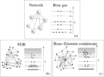
FIG. 30.: Mapping between the network model and the Bose gas. (a) On the left we have a network of five nodes, each characterized by a fitness $\eta_{i}$. Equation $(\ref{etaep})$ assigns an energy $\epsilon_{i}$ to each $\eta_{i}$ (right). An edge from node $i$ to node $j$ corresponds to a particle at level $\epsilon_{i}$ and one at $\epsilon_{j}$. The network evolves by adding a new node (dashed circle, $\eta_{6}$) which connects to $m=2$ other nodes (dashed lines), chosen following $(\ref{pi})$. In the gas this results in the addition of a new energy level ($\epsilon_{6}$, dashed) populated by $m=2$ new particles (open circles), and the deposition of $m=2$ other particles to energy levels to which the new node is connected to ($\epsilon_{2}$ and $\epsilon_{5}$). (b) In the FGR phase we have a continuous degree distribution, the several high degree nodes linking the low degree nodes together. In the energy diagram this corresponds to a decreasing occupation number with increasing energy. (c) In the Bose-Einstein condensate the fittest node attracts a finite fraction of all edges, corresponding to a highly populated ground level, and sparsely populated higher energies. After Bianconi and Barabási (2000b).

The continuum theory predicts that the rate at which particles accumulate on energy level $\epsilon_{i}$ is given by

$$\frac{\partial k_{i}(\epsilon_{i},t,t_{i})}{\partial t}=m\frac{e^{-\beta\epsilon_{i}}k_{i}(\epsilon_{i},t,t_{i})}{Z_{t}},$$ (133)

where $k_{i}(\epsilon_{i},t,t_{i})$ is the occupation number of level $i$ and $Z_{t}$ is the partition function, defined as $Z_{t}=\sum_{j=1}{t}e^{-\beta\epsilon_{j}}k_{j}(\epsilon_{j},t,t_{j})$. The solution of Eq. (133) is

$$k_{i}(\epsilon_{i},t,t_{i})=m\left(\frac{t}{t_{i}}\right)^{f(\epsilon_{i})},$$ (134)

where the dynamic exponent $f(\epsilon)$ satisfies $f(\epsilon)=e^{-\beta(\epsilon-\mu)}$, $\mu$ plays the role of the chemical potential, satisfying the equation

$$\int\deg(\epsilon)\frac{1}{e^{\beta(\epsilon-\mu)}-1}=1,$$ (135)

and $deg(\epsilon)$ is the degeneracy of the energy level $\epsilon$. Eq. (135) suggests that in the $t\rightarrow\infty$ limit the occupation number, giving the number of particles with energy $\epsilon$, follows the familiar Bose statistics

$$n(\epsilon)=\frac{1}{e^{\beta(\epsilon-\mu)}-1}.$$ (136)

The existence of the solution (134) depends on the functional form of the distribution $g(\epsilon)$ of the energy levels, determined by the $\rho(\eta)$ fitness distribution (see Sect. VIII.E.1). Specifically, if Eq. (135) has no nonnegative solution for a given $g(\epsilon)$ and $\beta$, we can observe a Bose-Einstein condensation, indicating that a finite fraction of the particles condensate on the lowest energy level (see Fig. 30c).

This mapping to a Bose gas predicts the existence of two distinct phases as a function of the energy distribution. In the fit-get-rich (FGR) phase, describing the case of uniform fitness discussed in Sect. VIII.E.1, the fitter nodes acquire edges at a higher rate than older but less fit nodes. In the end the fittest node will have the most edges, but the richest node is not an absolute winner, since its share of the edges (i.e. the ratio of its edges and the total number of edges in the network) decays to zero for large system sizes (Fig. 30b). The unexpected outcome of this mapping is the possibility of a Bose-Einstein condensation for $T<T_{BE}$, when the fittest node acquires a finite fraction of the edges, and maintains this share of edges over time (Fig. 30c). A representative fitness distribution which leads to condensation is $\rho(\eta)=(1-\eta)^{\lambda}$ with $\lambda>1$.

The temperature in (131) plays the role of a dummy variable, since if we define a fixed distribution $\rho(\eta)$, the existence of a Bose-Einstein condensation or the fit-get-rich phase depends only on the functional form of $\rho(\eta)$ and is independent of $\beta$. Indeed, $\beta$ falls out at the end from all topologically relevant quantities. As Dorogovtsev and Mendes (2000d) have subsequently shown, the existence of Bose-Einstein condensation can be derived directly from the fitness model, without employing the mapping to a Bose gas. While the condensation phenomenon appears to be similar to the gelation process observed by Krapivsky, Redner and Leyvraz (2000a) superlinear preferential attachment, it is not clear at this point if this similarity is purely accidental or there is a deeper connection between the fitness model and the fitness-free superlinear model.

IX ERROR AND ATTACK TOLERANCE

Many complex systems display a surprising degree of tolerance against errors. For example, relatively simple organisms grow, persist and reproduce despite drastic pharmaceutical or environmental interventions, an error tolerance attributed to the robustness of the underlying metabolic and genetic network (Jeong et al. 2000, 2001). Complex communication networks display a high degree of robustness: while key components regularly malfunction, local failures rarely lead to the loss of the global information-carrying ability of the network. The stability of these and other complex systems is often attributed to the redundant wiring of their underlying network structure. But could the network topology, beyond redundancy, play a role in the error tolerance of such complex systems?

While error tolerance and robustness almost always has a dynamical component, here we will focus only on the topological aspects of robustness, caused by edge and/or node removal. The first results regarding network reliability under edge removal came from random graph theory (Moore and Shannon 1956a,b, Margulis 1974 and Bollobás 1985). Consider an arbitrary connected graph $H_{N}$ of $N$ nodes, and assume that a $p$ fraction of the edges have been removed. What is the probability that the resulting subgraph is connected, and how does it depend on the removal probability $p$? For a broad class of starting graphs $H_{N}$ (Margulis 1974) there exists a threshold probability $p_{c}(N)$ such that if $p<p_{c}(N)$ the subgraph is connected, but if $p>p_{c}(N)$ it is disconnected. This phenomenon is in fact an inverse bond percolation problem defined on a graph, with the slight difference (already encountered in the evolution of a random graph) that the critical probability depends on $N$.

As the removal of a node implies the malfunctioning of all of its edges as well, node removal inflicts more damage than edge removal. Does a threshold phenomenon appear for node removal too? And to what degree does the topology of the network determine the network’s robustness? In the following we will call a network error tolerant (or robust) if it contains a giant cluster comprised of most of the nodes even after a fraction of its nodes are removed. The results indicate a strong correlation between robustness and network topology. In particular, scale-free networks are more robust than random networks against random node failures, but are more vulnerable when the most connected nodes are targeted.

A Numerical results

To compare the robustness of the Erdős-Rényi random graph and the scale-free model, Albert, Jeong and Barabási (2000) investigated networks that have the same number of nodes and edges, differing only in the degree distribution. Two types of node removal were considered. Random perturbations can cause the failure of some nodes, thus the first mechanism studied was the removal of randomly selected nodes. The second mechanism, in which the most highly connected nodes are removed at each step, was selected because it is the most damaging to the integrity of the system. This second choice emulates an intentional attack on the network.

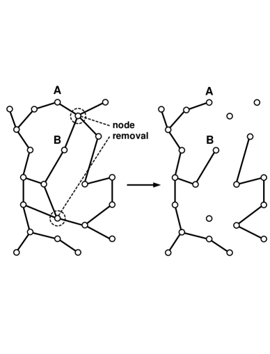
FIG. 31.: Illustration of the effects of node removal on an initially connected network. In the unperturbed state the distance between node A and B is $2$, but after two nodes are removed from the system, it increases to $6$. In the same time the network breaks into five isolated clusters.

Let us start from a connected network, and at each timestep remove a node. The disappearance of the node implies the removal of all edges that connect it to it, disrupting some of the paths between the remaining nodes. One way to monitor the disruption of an initially connected network is to study the relative size of the largest cluster that remains connected, $S$, and the average path length $\ell$ of this cluster, in function of the fraction $f$ of the nodes removed from the system. We expect that the size of the largest cluster decreases and its average path length increases as an increasing number of nodes are removed from the network.

1 Random network, random node removal

We start by investigating the response of a random network to the random removal of its nodes (see Fig. 32a, squares), looking at the changes in the relative size of the largest cluster, $S$ (i.e. the fraction of nodes contained in the largest cluster), and its average path length, $\ell$, as an increasing number of nodes are randomly removed.

The size of the largest cluster: As expected, for a random network $S$ decreases from $S=1$ as $f$ increases. If only the removed nodes would be missing from the largest cluster, $S$ would follow the diagonal corresponding to $S=1$ for $f=0$ and $S=0$ for $f=1$. While for small $f$, $S$ follows this line, as $f$ increases the decrease becomes more rapid, indicating that clusters of nodes become isolated from the main cluster. At a critical fraction $f_{c}$, $S$ drops to $0$, indicating that the network breaks into tiny isolated clusters. These numerical results indicate an inverse percolation transition. Indeed, percolation theory can be used to calculate the critical fraction $f_{c}$ (Sect. IX.B).

The average path length: The behavior of $\ell$ also confirms this percolation-like transition: it starts from the value characteristic to an unperturbed random graph; increases with $f$ as paths are disrupted in the network, and it peaks at $f_{c}$ (Fig. 32c, filled squares). After the network breaks into isolated clusters $\ell$ decreases as well since in this regime the size of the largest cluster decreases very rapidly.

FIG. 32.: The relative size $S$ (a, b) and average path length $\ell$ (c, d) of the largest cluster in an initially connected network when a fraction $f$ of the nodes are removed. (a, c) Erdős-Rényi random network with $N=10,000$ and $\langle k\rangle=4$. (b, d) Scale-free network generated by the scale-free model with $N=10,000$ and $\langle k\rangle=4$. Squares indicate random node removal, while circles correspond to preferential removal of the most connected nodes. After Albert, Jeong, Barabási (2000).

When $f$ is small we can use the prediction of random graph theory, (16), indicating that $\ell$ scales as $\log(SN)/\log(\langle k\rangle)$, where $\langle k\rangle$ is the average degree of the largest cluster (Sect. IV.G). Since the number of edges decreases more rapidly than the number of nodes during node removal (the disruption of each node inducing the disruption of several edges), $\langle k\rangle$ decreases faster with increasing $f$ than $SN$, and consequently $\ell$ increases. On the other hand, for $f\simeq f_{c}$ the prediction of percolation theory becomes valid, and Eq. (44) indicates that $\ell$ does not depend on $\langle k\rangle$ any longer, and decreases with $S$.

2 Scale-free network, random node removal

While a random network undergoes an inverse percolation transition when a critical fraction of its nodes are randomly removed, the situation is dramatically different for the SF network (Fig. 32b, d, squares). Simulations indicate that while the size of the largest cluster decreases, it reaches $0$ at a higher $f$. In the same time, $\ell$ increases much slower than in the random case, and its peak is much less prominent. The behavior of the system still suggests a percolation transition, but analytical calculations indicate that this is merely a finite size effect, and $f_{c}\rightarrow 1$ for a scale-free network as the size of the network increases (Sect. IX.B). In simple terms, scale-free networks display an exceptional robustness against random node failures.

3 Preferential node removal

In the case of an intentional attack, when the nodes with the highest number of edges are targeted, the network breaks down faster than in the case of random node removal. The general breakdown scenario follows again an inverse percolation transition, but now the critical fraction is much lower than in the random case. This is understandable, since at every step the highest possible number of edges are removed from the system. Again, the two network topologies respond differently to attacks (Fig. 32, circles): the scale-free network, due to its reliance on the highly connected nodes, breaks down earlier than the random network.

In conclusion, the numerical simulations indicate that scale-free networks display a topological robustness against random node failures. The origin of this error tolerance lies in their heterogeneous topology: low degree nodes are far more abundant than nodes with high degree, thus random node selection will more likely affect the nodes that play a marginal role in the overall network topology. But the same heterogeneity makes scale-free networks fragile to intentional attacks, since the removal of the highly connected nodes has a dramatic disruptive effect on the network.

B Error tolerance: analytical results

The critical threshold for fragmentation, $f_{c}$, of a network under random node failures was first calculated by Cohen et al. (2000) and Callaway et al. (2000). Cohen et al. (2000a) argue that for a random network with a given degree distribution $f_{c}$ can be determined using the following criterion: a giant cluster, with size proportional to the size of the original network, exists if an arbitrary node $i$, connected to a node $j$ in the giant cluster, is also connected to at least one other node. If $i$ is connected only to $j$, the network is fragmented. If we assume that loops can be neglected (true for large fragmented systems), this criterion can be written as

$$\frac{\langle k^{2}\rangle}{\langle k\rangle}=2.$$ (137)

Consider a node with initial degree $k_{0}$ chosen from an initial distribution $P(k_{0})$. After the random removal of a fraction $f$ of the nodes the probability that the degree of that node becomes $k$ is $C_{k_{0}}^{k}(1-f)^{k}f^{k_{0}-k}$, and the new degree distribution is

$$P(k)=\sum_{k_{0}=k}^{\infty}P(k_{0})C_{k_{0}}^{k}(1-f)^{k}f^{k_{0}-k}.$$ (138)

Thus the average degree and its second moment for the new system follows $\langle k\rangle=\langle k_{0}\rangle(1-f)$ and $\langle k^{2}\rangle=\langle k_{0}^{2}\rangle(1-f)^{2}+\langle k_{0}\rangle f(1-f)$, allowing us to rewrite the criterion (137) for criticality as

$$f_{c}=1-\frac{1}{\frac{\langle k_{0}^{2}\rangle}{\langle k_{0}\rangle}-1},$$ (139)

where $f_{c}$ is the critical fraction of removed nodes and $\langle k_{0}^{2}\rangle$, $\langle k_{0}\rangle$ are computed from the original distribution before the node removal.

Random graphs: As a test of the applicability of Eq. (137), let us remove a fraction $f$ of the nodes from a random graph. Since in the original graph $k_{0}=pN$ and $k_{0}^{2}=(pN)^{2}+pN$ (see Sect. III.C), Eq. (139) implies that $f_{c}=1-1/(pN).$ If in the original system $\langle k_{0}^{2}\rangle/\langle k_{0}\rangle=2$, meaning that $pN=\langle k\rangle=1$ (the familiar condition of the appearance of the giant cluster in a random graph), the above equation indicates that $f_{c}=0$, i.e. any amount of node removal leads to the network’s fragmentation. The higher the original degree $\langle k_{0}\rangle$ of the network, the larger the damage it can survive without breaking apart.

Scale-free networks: The critical probability is rather different if the degree distribution follows a power-law

$$P(k)=ck^{-\gamma},\quad\quad k=m,m+1,...K,$$ (140)

where $m$ and $K\simeq mN^{1/\gamma-1}$ are the smallest and the largest degree values, respectively. Using a continuum approximation valid in the limit $K\gg m\gg 1$, we obtain that

$$\frac{\langle k_{0}^{2}\rangle}{\langle k_{0}\rangle}\rightarrow\frac{|2-\gamma|}{|3-\gamma|}\times\left\{\begin{array}[]{lll}m&\mbox{if}&\gamma>3;\\ m^{\gamma-2}K^{3-\gamma},&\mbox{if}&2<\gamma<3;\\ K&\mbox{if}&1<\gamma<2.\end{array}\right.$$ (141)

We can see that for $\gamma>3$ the ratio is finite and there is a transition at

$$f_{c}=1-\frac{1}{\frac{\gamma-2}{\gamma-3}m-1}.$$ (142)

However, for $\gamma<3$ Eq. (141) indicates that the ratio diverges with $K$ and thus $f_{c}\rightarrow 1$ when $N\rightarrow\infty$. This result implies that infinite systems do not break down under random failures, as a spanning cluster exists for arbitrarily large $f$. In finite systems a transition is observed, although the transition threshold is very high. This result is in agreement with the numerical results discussed in the previous subsection (Albert, Jeong and Barabási 2000) indicating a delayed and very small peak in the $\ell$ curve for the failure of the SF model (having $\gamma=3$).

FIG. 33.: The fraction of nodes in the giant cluster, $S$, as a function of the fraction of randomly removed nodes for scale-free random networks with $\gamma=3.5$ (crosses) and $\gamma=2.5$ (all other symbols). In the latter case three different system sizes were used, with corresponding largest degree values $K=25$ (circles), $K=100$ (squares) and $K=400$ (triangles). The different curves illustrate that the fragmentation transition exists only for finite networks, while $f_{c}\rightarrow 1$ as $N\rightarrow\infty$. After Cohen et al. 2000

Callaway et al. (2000) investigate percolation on generalized random networks, considering that the occupation probability of nodes is coupled to the node degree. The authors use the method of generating functions discussed in Sect. V.B and generalize it to include the probability of occupancy of a certain node. The generating function for the degree distribution, corresponding to Eq. (46) in Sect. V.B, becomes

$$F_{0}(x)=\sum_{k=0}^{\infty}P(k)q_{k}x^{k},$$ (143)

where $q_{k}$ stands for the probability that a node with degree $k$ is present. The overall fraction of nodes which are present in the network is $q=F_{0}(1)$ which is also equal to $1-f$ where $f$ is the fraction of nodes missing from the system. This formulation includes the random occupancy (or conversely, random failure) case as the special case of uniform occupation probability $q_{k}=q$.

The authors consider random networks with a truncated power-law degree distribution

$$P(k)=\left\{\begin{array}[]{lcl}0&\mbox{for}&k=0\\ Ck^{-\gamma}e^{-k/\kappa}&\mbox{for}&k\geq 1\end{array}\right.$$ (144)

The exponential cutoff of this distribution has the role of regularizing the calculations in the same way as the largest degree $K$ in the study of Cohen et al. (2000).

In the case of uniform occupation probability $q$ corresponding to the random breakdown of a fraction $f=1-q$ of the nodes, the critical occupation probability follows

$$q_{c}=1-f_{c}=\frac{1}{\frac{Li_{\gamma-2}(e^{-1/\kappa})}{Li_{\gamma-1}(e^{-1/\kappa})}-1}.$$ (145)

Here $Li_{n}(x)$ is the $n$th polylogarithm of $x$, defined as $Li_{n}(x)=\sum_{k=1}^{\infty}x^{k}/k^{n}$. This expression is similar with Eq. (142) derived by Cohen et al., but we can notice that in contrast with Eq. (142), which is valid for $\gamma>3$, this equation gives nonzero values even for $2<\gamma<3$. The origin of the discrepancy is the cutoff $\kappa$ which captures the effects of size and capacity constrains (see Sect. VIII.D). Indeed, if we consider $\kappa\rightarrow\infty$, the expression for the critical occupation probability becomes

$$q_{c}=\frac{1}{\frac{\zeta(\gamma-2)}{\zeta(\gamma-1)}-1},$$ (146)

where $\zeta(x)$ is the Riemann $\zeta$ function defined in the region $x>1$, thus this expression is valid only for $\gamma>3$. Since $\zeta(x)\rightarrow\infty$ as $x\rightarrow 1$, $q_{c}$ becomes zero as $\gamma$ approaches $3$, indicating that for infinite scale-free networks even infinitesimal occupation probabilities can assure the presence of an infinite cluster.

C Attack tolerance: analytical results

In the general framework of Callaway et al. (2000), intentional attack targeted at the nodes with highest degree is equivalent with setting

$$q_{k}=\theta(k_{max}-k)=\left\{\begin{array}[]{lcl}1&\mbox{if}&k\leq k_{max}\\ 0&\mbox{if}&k>k_{max}\end{array}\right..$$ (147)

This way only the nodes with degree $k\leq k_{max}$ are occupied, which is equivalent with removing all nodes with $k>k_{max}$. The number of removed nodes can be increased by lowering the value of $k_{max}$. Callaway et al. (2000) calculate the fraction of nodes in the infinite cluster $S$ as a function of $f$ and $k_{max}$ (Fig. 34). This figure is in agreement with the results of Albert et al. (2000) indicating that scale-free networks become fragmented after a small fraction $f_{c}$ of highly connected nodes is removed. It also indicates that a small percentage of the highest connected nodes contains in fact nodes with surprisingly low degree, agreeing also with the finding of Broder et al. (2000) that the World-Wide Web is resilient to the removal of all nodes with degree higher than $5$.

FIG. 34.: Fraction of nodes in the spanning cluster in scale-free random networks with all nodes with degree greater than $k_{max}$ unoccupied, for $\gamma=2.4$ (circles), $\gamma=2.7$ (squares) and $\gamma=3.0$ (triangles). The solid lines are the analytical prediction. Upper frame: as a function of $f$. Lower frame: as a function of the cutoff $k_{max}$. After Callaway et al. 2000.

The theoretical framework of Cohen et al. (2000) can also be extended to the case of intentional attack on a scale-free network with degree distribution (140) (Cohen et al. 2001). Under attack two effects arise: (a) the cutoff degree $K$ is reduced to a new value $\tilde{K}<K$, and (b) the degree distribution of the remaining nodes is changed. The new cutoff can be estimated from the relation

$$\sum_{k=\tilde{K}}^{K}P(k)=\sum_{k=\tilde{K}}^{\infty}P(k)-\frac{1}{N}=f,$$ (148)

which for large $N$ implies

$$\tilde{K}=mf^{1/(1-\gamma)}.$$ (149)

The removal of a fraction $f$ of the most connected nodes results in a random removal of a fraction $\tilde{f}$ of edges from the remaining nodes. The probability that an edge leads to a deleted node equals the fraction of edges belonging to deleted nodes

$$\tilde{f}=\frac{\sum_{k=\tilde{K}}^{K}kP(k)}{\langle k_{0}\rangle}=f^{(2-\gamma)/(1-\gamma)},$$ (150)

for $\gamma>2$. In the limit $\gamma=2$, $\tilde{f}=\ln(Nf/m)$, thus very small $f$ values can lead to the destruction of a large fraction of the edges as $N\rightarrow\infty$.

Since for random node deletion the probability of an edge leading to a deleted node equals the fraction of deleted nodes, Cohen et al. (2001) argue that the network after undergoing an attack is equivalent with a scale-free network with cutoff $\tilde{K}$ that has undergone random removal of a fraction $\tilde{f}$ of its nodes. Replacing $f$ with $\tilde{f}$ and $K$ with $\tilde{K}$ in Eq. (139), we obtain the following equation for $\tilde{K}$:

$$\left(\frac{\tilde{K}}{m}\right)^{2-\gamma}-2=\frac{2-\gamma}{3-\gamma}m\left[\left(\frac{\tilde{K}}{m}\right)^{3-\gamma}-1\right].$$ (151)

This equation can be solved numerically to obtain $\tilde{K}$ as a function of $m$ and $\gamma$, then $f_{c}(m,\gamma)$ can be determined from (149). The results indicate that a breakdown phase transition exists for $\gamma>2$, and $f_{c}$ is very small for all $\gamma$ values, on the order of a few percent. An interesting feature of the $f_{c}(\gamma)$ curve is that it has a maximum around $\gamma=2.25$. It is not surprising that smaller $\gamma$ values lead to increased vulnerability to attacks due to the special role the highly connected nodes play in connecting the system. On the other hand, Cohen et al. (2001) argue that the cause of the increased susceptibility of high $\gamma$ networks is that for these even the original network is formed by several independent clusters, and the size of the largest cluster decreases with increasing $\gamma$. Indeed, the results of Aiello, Chung and Lu (2000) (see Sect.V) indicate that for $2<\gamma<3.478$ the original network contains an infinite cluster and several smaller clusters of size at most $\log N$ and for $\gamma>3.478$ the original network has no infinite cluster.

D The robustness of real networks

Systematic studies on error and attack tolerance of real networks are available for four systems highly relevant to science an technology.

Communication networks: The error and attack tolerance of the Internet and the WWW was investigated by Albert, Jeong and Barabási (2000). Of the two networks, the Internet’s robustness has more practical significance, as about $0.3\%$ of the routers regularly malfunction (random errors), and the Internet is occasionally subject to hacker attacks targeting some of the most connected nodes. The results, based on the latest map of the Internet topology at the inter-domain (autonomous system) level, indicate that the average path length on the Internet is unaffected by the random removal of as many as $60\%$ of the nodes, while if the most connected nodes are eliminated (attack), $\ell$ peaks at a very small $f$ (Fig. 35a). Similarly, the large connected cluster persists for high rates of random node removal, but if nodes are removed in the attack mode, the size of the fragments that break off increases rapidly, the critical point appearing at a very small threshold, $f_{c}^{I}\simeq 0.03$ (Fig. 35c).

FIG. 35.: The relative size $S$ (a, b) and average path length $\ell$ (c, d) of the largest cluster in two communication networks when a fraction $f$ of the nodes are removed. (a, c), Internet at the domain level, $N=6,209$, $\langle k\rangle=3.93$. (b, d) Subset of the WWW with $N=325,729$ and $\langle k\rangle=4.59$. Squares indicate random node removal, circles mean preferential removal of the most connected nodes. After Albert, Jeong, Barabási 2000.

The WWW study was limited to a subset of the web containing $325,729$ nodes, the sample investigated in Albert, Jeong and Barabási (1999). As the WWW is directed, not all nodes can be reached from all nodes even for the starting network. To resolve this problem, only distances between nodes that have a path between them are included in the average distance between nodes. Second, directed networks cannot be separated into clusters unambiguously: two nodes can be seen as part of the same cluster when starting from a certain node, and appear to be in separate clusters when starting from another. This way the number of independent clusters is not unambiguous, but the largest cluster can be determined. Third, when simulating an attack on the WWW, the nodes with the highest number of outgoing edges were removed, since $k_{out}$ can be readily obtained by looking on a web document, while $k_{in}$ can be only determined when the map of the whole web is available. Despite these methodological differences, the response of the WWW is similar to the undirected networks: after a slight initial increase, $\ell$ remains constant in the case of random failures (Fig. 35b), while it increases for attacks. The network survives as a large cluster under high rates of failure, but under attack the system abruptly falls apart at $f_{c}^{w}=0.067$ (Fig. 35d).

Cellular networks: Cellular networks can be subject to random errors as a result of mutations or protein misfolding, as well as harsh external conditions eliminating essential metabolites. Jeong et al. (2000) study the response of the metabolic networks of several organisms to random and preferential node removal. Removing up to $8\%$ of the substrates they obtain that the average path length does not increase when the nodes are removed randomly, but it increases rapidly under the removal of the most connected nodes, attaining a $500\%$ increase with the removal of only $8\%$ of the nodes. Similar results have been obtained for the protein network of yeast as well (Jeong et al. 2001, see also Vogelstein, Lane and Levine 2000).

Ecological networks: As a result of human actions or environmental changes, species are deleted from food webs, an issue of major concern for ecology and environmental science. Solé and Montoya (2000) study the response of the food webs discussed in Sect. II to the removal of species (nodes) (Montoya and Solé 2000). The authors measure the relative size $S$ of the largest cluster, the average size $\langle s\rangle$ of the rest of the species clusters, and the fraction of species becoming isolated due to removal of other species on whom their survival depends (secondary extinctions). The results indicate that under random species removal the fraction of species contained in the largest cluster decreases linearly. In the same time the values of $\langle s\rangle$ remain $0$ or $1$, and the secondary extinction rates remain very low (smaller than $0.1$) even when a high fraction of the nodes is removed. The estimate of Eq. (139) for the critical fraction at which the network fragments gives $f_{c}^{fail}$ values around $0.95$ for all networks, indicating that these networks are error tolerant. However, when the most connected (keystone) species are successively removed, $S$ decays quickly and becomes zero at $f_{c}^{attack}\simeq 0.2$, while $\langle s\rangle$ peaks. The secondary extinctions increase dramatically, reaching $1$ at relatively low values of $f$ ($f\simeq 0.16$ for the Silwood Park web).

The results presented in this section offer a simple but compelling picture: scale-free networks display a high degree of robustness against random errors, coupled with a susceptibility to attacks. This double feature is the result of the heterogeneity of the network topology, encoded by the power-law degree distribution. While we focused on two measures only, $S$ and $\ell$, it is likely that most network measures will show distinct behavior for scale-free and random networks.

The type of disturbances we considered were static, that is, the removal of a node affected other nodes only in the topological sense. On the other hand, in many networks there is a dynamical aspect to error tolerance: the removal of a node could affect the functionality of other nodes as well. For example, the removal of a highly connected router on the Internet will redirect traffic to other routers that may not have the capacity to handle the increased traffic, creating an effective denial of service attack. Thus in many systems errors lead to cascading failures, affecting a large fraction of the network. While little is known about such events, Watts (2001) has recently shown that the network topology makes a big difference under cascading failures as well. He investigated a binary model in which the state of a node changes from off to on if a threshold fraction of its neighbors are on. In this model the probability that a perturbation in an initially all-off state spreads to the entire network can be connected to the existence of a giant cluster of vulnerable nodes. Using the method of generating functions, Watts (2001) showed that scale-free random graphs are much less vulnerable to random perturbations than Erdős-Rényi random graphs with the same average degree.

It is often assumed that the robustness of many complex systems is rooted in their redundancy, which for networks represents the existence of many alternative paths that can preserve communication between nodes even if some nodes are absent. We are not aware of any research that would attempt to address this issue in quantitative terms, uncovering to which degree does redundancy play a role.

X OUTLOOK

Just like its main subject, the field of complex networks is rapidly evolving. While the potential for new and important discoveries is high, it has attained a degree of coherence that made a review necessary and appropriate. The fact that the obtained results have reached a critical mass is best illustrated by the amount of work that we had no space to review above. Being forced to make a choice, we focused on the mechanisms and models that describe network topology. In the following we briefly discuss the results that could not fit in this approach, but are important for the field. In many ways the list is as prominent as the works covered so far.

1 Dynamics on networks

Most networks offer a support for various dynamical processes, as often the topology plays a crucial role in determining the system’s dynamical features. The range of possible dynamical processes is wide. Watts (1999) studied the impact of clustering on several processes, including games, cooperation, the Prisoner’s Dilemma, cellular automata and synchronization (see also Lago-Fernández et al. 2001). Wang and Chen (2001) have shown that inhomogeneous scale-free topology plays an important role in determining synchronization on a complex network, but search and random walks on complex networks is also a much investigated topic (Huberman et al. 1998, Kleinberg 2000, Adamic et al. 2001, Burda et al. 2001, Walsh 2001, Bilke and Peterson 2001). Modeling dynamics on a fixed topology is legitimate when the timescales describing the network topology and the dynamics on the network differ widely. A good example is Internet traffic, whose modeling requires time resolutions from milliseconds up to a day (Willinger et al. 1997, Crovella and Bestavros 1997, Solé and Valverde 2001), compared with the months required for significant topological changes. Similarly, within the cell the concentrations of different chemicals change much faster than the cellular network topology (Schilling and Palsson 1998, Savageau 1998, Gardner et al. 2000, Elowitz and Leibler 2000), which is shaped by evolution over many generations.

The network structure plays a crucial role in determining the spread of ideas, innovations or computer viruses (Coleman, Menzel and Katz 1957, Valente 1995). In this light, spreading and diffusion has been studied both on regular (Kauffman 1992, Keeling 1999), random (Solomonoff, Rapoport 1951, Rapoport 1957, Weigt and Hartmann 2001), small-world (Abramson and Kuperman 2000, Newman and Watts 1999, Moukarzel 1999, Newman, Moore, Watts 2000, Moore and Newman 2000a,b) and scale-free (Johansen and Sornette 2000, Watts 2001, Bilke and Peterson 2001 ,Tadić 2001b) networks. A particularly surprising result was offered recently by Pastor-Satorras and Vespignani (2001a,b), who studied the effect of the network topology on disease spreading. They show that while for random networks a local infection spreads to the whole network only if the spreading rate is larger than a critical value $\lambda_{c}$, for scale-free networks any spreading rate leads to the infection of the whole network. That is, for scale-free networks the critical spreading rate reduces to zero, a highly unexpected result that goes against volumes of results written on this topic.

When the timescales governing the dynamics on the network are comparable to that characterizing the network assembly, the dynamical processes can influence the topological evolution. This appears to be the case in various biological models inspired by the evolution of communities or the emergence of the cellular topology (Slanina and Kotrla 1999, 2000, Bornholdt and Sneppen 2000, Jain and Krishna 2001, Lässig et al. 2001). In the current models often these systems are not allowed to ”grow”, but they exist in a stationary state that gives room for diverse network topologies (Slanina and Kotrla 1999, 2000). Interestingly, these models do not lead to scale-free networks in the stationary state, while it is known that cellular networks are scale-free (Jeong et al. 2000, 2001, Wagner and Fell 2000). Thus it is an open challenge to design evolutionary models that, based on selection or optimization mechanisms, could produce topologies similar to those seen in the real world.

In general, when it comes to understanding dynamics on networks, as well as the coupling between the dynamics and network assembly, we are only at the beginning of a promising journey (Strogatz 2001). So far we are missing simple organizing principles that would match the coherence and universality characterizing network topology. Due to the importance of the problem, and the rapid advances we witnessed in descibing network topology, we foresee it as being a rapidly growing area.

2 Directed networks

Many important networks, including the WWW or metabolic networks, have directed edges. In directed networks, however, not all nodes can be reached from a given node. This leads to a fragmented cluster structure, where the clusters are not unique, but they depend on the starting point of the inquiry. Beyond some general aspects, little is known about such directed networks, but important insights could emerge in the near future. A promising step in this direction is the empirical study of the cluster structure of the World-Wide Web (Broder et al. 2000), finding that the WWW can be partitioned into several qualitatively different domains. The results indicate that $28\%$ of the nodes are part of the strongly connected component (SCC), in which any pair of nodes is connected by paths in either direction. Another $23\%$ of the nodes can be reached from the SCC, but cannot connect to it in the other direction, while a roughly equal fraction of the nodes have paths leading to the SCC but cannot be reached from it. As several groups have pointed out, this structure is not specific to the WWW, but common to all directed networks, ranging from the cell metabolism to citation networks (Newman, Strogatz and Watts 2000, Dorogovtsev, Mendes and Samukhin 2001).

Most network models (including small world and evolving networks) ignore the network’s directedness. On the other hand, as the WWW measurements have shown, the incoming and outgoing edges could follow different scaling laws. In this respect, the scale-free model (Barabási and Albert 1999) explains only the incoming degree distribution, as, due to its construction, each node has exactly $m$ outgoing edges, thus the outgoing degree distribution is a delta function (Sect. VII.A). While recently several models have investigated directed evolving networks, obtaining a power-law for both the outgoing and incoming edges (Tadić 2001a,b, Krapivsky, Rodgers, Redner 2001), the generic features of such complex directed models could hold further surprises.

3 Weighted networks, optimization, allometric scaling

Many real networks are weighted networks, in contrast with the binary networks investigated so far, where the edge weights can have only two values $0$ and $1$ (absent or present). Indeed, in social networks it is often important to assign a strength to each acquaintance edge, indicating how well the two individuals know each other (Newman 2001b,c). Similarly, cellular networks are characterized by reaction rates, and the edges on the Internet by bandwidth. What are the mechanisms that determine these weights? Do they obey nontrivial scaling behavior? To what degree are they determined by the network topology? Most answers to these questions come from two directions: theoretical biology and ecology, concerned with issues related to allometric scaling, and random resistor networks (Derrida and Vannimenus 1982, Duxbury, Beale and Moukarzel 1995), a topic much studied in statistical mechanics. Allometric scaling describes the transport of material through the underlying network characterizing various biological systems. Most of these systems have a branching tree-like topology. The combination of the tree topology with the desire to minimize the cost of transportation leads to nontrivial scaling in the weights of the edges (West et al. 1997, Enquist et al. 1998, 1999).

In a more general context, Banavar and collaborators have shown that when the aim is to minimize the cost of transportation, the optimal network topology can vary widely, ranging from tree-like structures to spirals or loop-dominated highly interconnected networks (Banavar at al. 1999, 2000). Beyond giving systematic methods and principles to predict the topology of transportation networks, these studies raise some important questions that need to be addressed in the future. For example, to which degree is the network topology shaped by global optimization, or the local processes seen in scale-free networks? There are fundamental differences between transportation and evolving networks. In transportation models the network topology is determined by a global optimization process, in which edges are positioned to minimize, over the whole network, some predefined quantity, such as cost or energy of transportation. In contrast, for evolving networks such global optimization is absent, as the decision where to link is delegated to the node level. However, this decision is not entirely local in scale-free networks either, as the node has information about the degree of all nodes in the network, from which it chooses one following (78), the normalization factor in making the system fully coupled. The interplay between such local and global optimization processes is far from being fully understood (Carlson and Doyle 1999, 2000, Doyle and Carlson 2000).

While edge weights are well understood for trees and some much studied physical networks, ranging from river networks (Rodríguez-Iturbe and Rinaldo 1997, Banavar et al. 1997) to random resistor networks (Derrida and Vannimenus 1982, Duxbury, Beale and Moukarzel 1995), little work is done on these problems in the case of small world or scale-free networks. Recently Yook et al. (2001) have investigated an evolving network model in which the weights were added dynamically, resulting in unexpected scaling behavior. Newman (2001b) has also assigned weights to characterize the collaboration strength between scientists. These studies make an important point, however: despite the practical relevance and potential phenomenological richness, the understanding of weighted networks is still in its infancy.

4 Internet and World-Wide Web

A few real networks, with high technological or intellectual importance, have received special attention. In these studies the goal is to develop models that go beyond the basic growth mechanisms and incorporate the specific and often unique details of a given system. Along these lines much attention has focused on developing realistic World-Wide Web models that explain everything from the average path length to incoming and outgoing degree distribution (Adamic, Huberman 1999, Flake et al. 2000, Tadić 2001a, Krapivsky, Rodgers, Redner 2001). Many studies focus on the identification of web communities as well, representing clusters of nodes that are highly connected to each other (Gibson et al. 1998, Flake et al. 2000, Pennock et al. 2000, Adamic and Adar 2000).

There is a race in computer science to create good Internet topology generators (Paxson, Floyd 1997, Comellas et al. 2000). New Internet protocols are tested on model networks before their implementation, and protocol optimization is sensitive to the underlying network topology (Labovitz et al. 2000). Prompted by the discovery that the Internet is a scale-free network, all topology generators are being reviewed and redesigned. These studies have resulted in careful investigations into what processes could contribute to the correct topology, reaffirming that growth and preferential attachment are necessary conditions for realistic Internet models (Medina et al. 2000, Palmer, Steffan 2000, Yook et al. 2001b, Pastor-Satorras et al 2001, Jeong, Néda, Barabási 2001). In addition, an interesting link has been recently found (Caldarelli et al. 2000) to river networks, a much studied topic in statistical mechanics (see Banavar et al. 1999, Dodds and Rothman 2000, 2001a,b,c).

5 General questions

The high interest in scale-free networks might give the impression that all complex networks in nature have power-law degree distributions. As we discussed in Sect. II, that is far from being the case. It is true that several complex networks of high interest for the scientific community, such as the WWW, cellular networks, Internet, some social networks and the citation network are scale-free. However, others like the power grid or the neural network of C. elegans appear to be exponential. Does that mean that they are random? Far from it. These systems are also best described by evolving networks. As we have seen in many examples in Sect. VIII, evolving networks can develop both power-law and exponential degree distributions. While the power-law regime appears to be robust, sublinear preferential attachment, aging effects, growth constraints lead to crossovers to exponential decay. Thus, while evolving networks are rather successful at describing a wide range of networks, the functional form of $P(k)$ cannot be guessed until the microscopic details of the network evolution are fully understood. If all processes shaping the topology of a certain network are properly incorporated, the resulting $P(k)$ often has a rather complex form, described by a combination of power-laws and exponentials.

In critical phenomena we are accustomed to unique scaling exponents that characterize complex systems. Indeed, the critical exponents are uniquely determined by robust factors, such as the dimension of the space or conservation laws (Stanley 1971, Ma 1976, Hohenberg and Halperin 1977). The most studied exponents in terms of evolving networks are the dynamic exponent, $\beta$ and the degree exponent $\gamma$. While the former characterizes the network dynamics, the latter is a measure of the network topology. The inseparability of the topology and the dynamics of evolving networks is shown by the fact that these exponents are related by the scaling relation (86) (Dorogovtsev, Mendes, Samukhin 2000a), underlying the fact that the network assembly uniquely determines the network topology. However, in no case are these exponents unique. They can be tuned continuously by such parameters as the frequency of internal edges, rewiring rates, initial node attractiveness and so on. While it is difficult to search for universality in the value of the exponents, this does not imply that the exponents are not uniquely defined. Indeed, if all processes contributing to the network assembly and evolution are known, the exponents can be calculated exactly. But they do not take up the discrete values we are accustomed to in critical phenomena.

Some real networks have an underlying bipartite structure (Sect. V.D). For example, the actor network can be represented as a graph consisting of two types of nodes: actors and movies, the edges always connecting two nodes of different type. These networks can be described as generalized random graphs (Newman, Strogatz and Watts 2000). It is important to note, however, that both subsets of these bipartite graphs are growing in time. While it has not been attempted yet, the theoretical methods developed for evolving networks can be generalized for bipartite networks as well, leading to coupled continuum equations. We expect that extending these methods, whenever appropriate, would lead to a much more realistic description of several real systems.

The classical thinking of complex networks, rooted in percolation and random graph theory (see Aldous 1999), is that they appear as a result of a percolation process in which isolated nodes eventually join a giant cluster as the number of edges increases between them. Thus a much studied question concerns the threshold at which the giant cluster appears. With a few exceptions (Callaway et al. 2001), evolving networks do not follow this percolation picture, since they are connected from their construction. Naturally, if node or edge removal is allowed, percolation-type questions do emerge (Sect. IX).

6 Conclusions

The shift that we experienced in the past three years in our understanding networks was rather swift and unexpected. We have learned through empirical studies, models and analytic approaches that real networks are far from being random, but display generic organizing principles shared by rather different systems. These advances have created a prolific branch of statistical mechanics, followed with equal interest by sociologists, biologists and computer scientists. Our goal here was to summarize, in a coherent fashion, what is known so far. Yet, we believe that these results are only the tip of the iceberg. We have uncovered some generic topological and dynamical principles, but the answers to the open questions could hide new concepts and ideas that might turn out to be equally exciting as those we encountered so far. The future could bring a new infusion of tools as well, as the recent import of ideas from field theory (Burda et al. 2001) and quantum statistics (Bianconi 2000a, Bianconi and Barabási 2000, Zizzi 2001) indicate. Consequently, this article is intended to be as much a review a catalyst for further advances. We hope that the latter aspect will dominate.

7 Acknowledgments

We wish to thank Altavista, István Albert, Alain Barrat, Ginestra Bianconi, Duncan Callaway, Reuven Cohen, Ramesh Govindan, José Mendes, Christian Moukarzel, Zoltán Néda, Mark Newman, Steven Strogatz, Andrew Tomkins and Duncan Watts for allowing us to reproduce their figures. We are grateful to Luis N. Amaral, Alain Barrat, Duncan Callaway, Reuven Cohen, Imre Derényi, Sergei Dorogovtsev, Illés Farkas, Shlomo Havlin, Miroslav Kotrla, Paul Krapivsky, José Mendes, Christian Moukarzel, Mark Newman, Sidney Redner, Frantisek Slanina, Ricard Solé, Steven Strogatz, Bosiljka Tadić, Tamás Vicsek and Duncan Watts for reading our manuscript and helpful suggestions. We have benefited from discussions with István Albert, Ginestra Bianconi, Zoltán Dezső, Hawoong Jeong, Zoltán Néda, Erzsébet Ravasz and Soon-Hyung Yook. This research was supported by NSF-DMR-9710998 and NSF-PHYS-9988674.

REFERENCES

- [1] Abello, J., P. M. Pardalos and M. G. C. Resende, 1999, DIMACS Series in Disc. Math. and Theor. Comp. Sci. 50, 119.
- [2] Adamic, L. A., 1999, Proceedings of the ECDL’99 Conference (Springer), 443.
- [3] Adamic, L. A. and E. Adar, 2000, preprint, www.parc.xerox.com/istl/groups/iea/papers/.
- [4] Adamic, L. A. and B. A. Huberman, 1999, Nature 401, 131.
- [5] Adamic, L. A. and B. A. Huberman, 2000, Science 287, 2115.
- [6] Adamic, L. A., R. M. Lukose, A. R. Puniyani and B. A. Huberman, 2001, arXiv:cs.NI/0103016.
- [7] Aiello, W., F. Chung and L. Lu, 2000, in Proc. nd ACM Symp. Theor. Comp.
- [8] Albert, R. and A.-L. Barabási, 2000, Phys. Rev. Lett. 85, 5234.
- [9] Albert, R., H. Jeong and A.-L. Barabási, 1999, Nature 401, 130.
- [10] Albert, R., H. Jeong and A.-L. Barabási, 2000, Nature 406, 378; Erratum, 2001, Nature 409, 542.
- [11] Aldous, D., 1999, Bernoulli 5, 3.
- [12] Amaral, L. A. N., M. Barthélémy and P. Gopikrishnan, 1999, unpublished.
- [13] Amaral, L. A. N., A. Scala, M. Barthélémy and H. E. Stanley, 2000, Proc. Nat. Acad. Sci. USA 97, 11149.
- [14] Argollo de Menezes, M., C. F. Moukarzel and T. J. P. Penna, 2000, Europhys. Lett. 50, 574.
- [15] Banavar, J. R., F. Colaiori, A. Flammini, A. Giacometti, A. Maritan and A. Rinaldo, 1997, Phys. Rev. Lett. 78, 4522.
- [16] Banavar, J. R., A. Maritan and A. Rinaldo, 1999, Nature 399, 130.
- [17] Banavar, J. R., F. Colaiori, A. Flammini, A. Maritan and A. Rinaldo, 2000, Phys. Rev. Lett. 84, 4745.
- [18] Barabási, A.-L. and R. Albert, 1999, Science 286, 509.
- [19] Barabási, A.-L., H. Jeong, E. Ravasz, Z. Néda, A. Schubert and T. Vicsek, 2001, arXiv:cond-mat/0104162.
- [20] Barabási, A.-L., R. Albert and H. Jeong, 1999, Physica A 272, 173.
- [21] Barrat, A., 1999, arXiv:cond-mat/9903323.
- [22] Barrat, A. and M. Weigt, 2000, Euro. Phys. Journ. B 13, 547.
- [23] Barthélémy, M. and L. A. N. Amaral, 1999, Phys. Rev. Lett. 82, 3180; Erratum, 1999, Phys. Rev. Lett 82, 5180.
- [24] ben Avraham, D. and S. Havlin, 2000, Diffusion and Reactions in Fractals and Disordered Systems (Cambridge University Press).
- [25] Bianconi, G., 2000, Int. J. Mod. Phys. B 14, 3356.
- [26] Bianconi, G. 2000b, unpublished.
- [27] Bianconi, G. and A.-L. Barabási, 2000a, cond-mat/0011029.
- [28] Bianconi, G. and A.-L. Barabási, 2000b, cond-mat/0011224.
- [29] Bilke, S. and C. Peterson, 2001, arXiv:cond-mat/0103361.
- [30] Bollobás, B., 1981, Discrete Math. 33, 1.
- [31] Bollobás, B., 1984, Trans. Amer. Math. Soc. 286, 257.
- [32] Bollobás, B., 1985, Random Graphs (Academic Press, London).
- [33] Bornholdt, S. and H. Ebel, 2000, arXiv:cond-mat/0008456.
- [34] Bornholdt, S. and K. Sneppen, 2000, arXiv:cond-mat/0003333.
- [35] Broder, A., R. Kumar, F. Maghoul, P. Raghavan, S. Rajalopagan, R. Stata, A. Tomkins and J. Wiener, 2000, Comput. Netw. 33, 309.
- [36] Bunde, A. and S. Havlin (eds.), 1994, Fractals in Science (Springer, Berlin).
- [37] Bunde, A. and S. Havlin (eds.), 1996, Fractals and Disordered Systems (Springer, Berlin).
- [38] Burda, Z., J. D. Correira and A. Krzywicki, 2001, arxiv:cond-mat/0104155.
- [39] Burton, R. M. and M. Keane, 1989, Comm. Math. Phys. 121, 501.
- [40] Caldarelli, G., R. Marchetti and L. Pietronero, 2000, Europhys. Lett. 52, 386.
- [41] Callaway, D. S., M. E. J. Newman, S. H. Strogatz and D. J. Watts, 2000, Phys. Rev. Lett. 85, 5468.
- [42] Callaway, D. S., J. E. Hopcroft, J. M. Kleinberg, M. E. J. Newman and S. H. Strogatz, 2001, arXiv:cond-mat/0104546.
- [43] Camacho, J., R. Guimerà and L. A. N. Amaral, 2001a, cond-mat/0102127.
- [44] Camacho, J., R. Guimerà and L. A. N. Amaral, 2001b, cond-mat/0103114.
- [45] Carlson, J. M. and J. Doyle, 1999, Phys. Rev. E 60, 1412.
- [46] Carlson, J. M. and J. Doyle, 2000, Phys. Rev. Lett. 84, 2529.
- [47] Christensen, K., R. Donangelo, B. Koiler, and K. Sneppen, 1998, Phys. Rev. Lett. 81, 2380.
- [48] Chung, F. and L. Lu, 2001, Adv. Appl. Math. (in press).
- [49] Cohen, J. E., 1988, Discr. Appl. Math. 19, 113.
- [50] Cohen, R., K. Erez, D. ben-Avraham and S. Havlin, 2000, Phys. Rev. Lett. 85, 4626.
- [51] Cohen, R., K. Erez, D. ben-Avraham and S. Havlin, 2001, Phys. Rev. Lett. 86, 3682.
- [52] Coleman, J. S., H. Menzel and E. Katz, 1957, Sociometry 20, 253.
- [53] Comellas, F., J. Ozon, J. G. Peters, 2000, Inform. Process. Lett. 76, 83.
- [54] Crisanti, A., G. Paladin and A. Vulpiani, 1993, Products of Random Matrices in Statistical Physics, (Springer, Berlin).
- [55] Crovella, M. E. and A. Bestavros, 1997, IEEE/ACM Transactions on Networking 5, 835.
- [56] Derrida, B., J. Vannimenus, 1982, J. Phys. A 15, L557.
- [57] Dodds, P. S. and D. H. Rothman, 2000, Annu. Rev. Planet. Sci. 28, 571.
- [58] Dodds, P. S. and D. H. Rothman, 2001a, Phys. Rev. E 63, 016115.
- [59] Dodds, P. S. and D. H. Rothman, 2001b, Phys. Rev. E 63, 016116.
- [60] Dodds, P. S. and D. H. Rothman, 2001c, Phys. Rev. E 63, 016117.
- [61] Dorogovtsev, S. N. and J. F. F. Mendes, 2000a, Europhys. Lett. 50, 1.
- [62] Dorogovtsev, S. N. and J. F. F. Mendes, 2000b, Phys. Rev. E 62, 1842.
- [63] Dorogovtsev, S. N. and J. F. F. Mendes, 2000c, Europhys. Lett 52, 33.
- [64] Dorogovtsev, S. N. and J. F. F. Mendes, 2000d, arXiv:cond-mat/0009065.
- [65] Dorogovtsev, S. N. and J. F. F. Mendes, 2001, arXiv:cond-mat/0105093.
- [66] Dorogovtsev, S. N., J. F. F. Mendes and A. N. Samukhin, 2000a, Phys. Rev. Lett. 85, 4633.
- [67] Dorogovtsev, S. N., J. F. F. Mendes and A. N. Samukhin, 2000b, arXiv:cond-mat/0009090.
- [68] Dorogovtsev, S. N., J. F. F. Mendes and A. N. Samukhin, 2000b, arXiv:cond-mat/0011077.
- [69] Dorogovtsev, S. N., J. F. F. Mendes and A. N. Samukhin, 2000c, arXiv:cond-mat/0011115.
- [70] Dorogovtsev, S. N., J. F. F. Mendes and A. N. Samukhin, 2001, arXiv:cond-mat/0103629.
- [71] Doyle, J. and J. M. Carlson, 2000, Phys. Rev. Lett. 84, 5656.
- [72] Durrett, R. T., 1985, Zeitschrift fur Wahrscheinlichkeitstheorie und Verwandte Gebiete 69, 421.
- [73] Duxbury, P. M., P. D. Beale and C. Moukarzel, 1995, Phys. Rev. B 51, 3476.
- [74] Elowitz, M. B. and S. Leibler, 2000, Nature 403, 335.
- [75] Enquist, B. J., J. H. Brown and G. B. West, 1998, Nature 395, 163.
- [76] Enquist, B. J., G. B. West, E. L. Charnov, and J. H. Brown, 1999, Nature 401, 907.
- [77] Erdős, P. and A. Rényi, 1959, Publ. Math. Debrecen 6, 290.
- [78] Erdős, P. and A. Rényi, 1960, Publ. Math. Inst. Hung. Acad. Sci 5, 17.
- [79] Erdős, P. and A. Rényi, 1961, Bull. Inst. Int. Stat. 38, 343.
- [80] Ergün, G. and G. J. Rodgers, 2001, arXiv:cond-mat/0103423.
- [81] Faloutsos, M., P. Faloutsos and C. Faloutsos, 1999, Proc. ACM SIGCOMM, Comput. Commun. Rev. 29, 251.
- [82] Farkas, I. J., I. Derényi, A.-L. Barabási and T. Vicsek, 2001, Phys. Rev. E (in press), arXiv:cond-mat/0102335.
- [83] Fell, D. A. and A. Wagner, 2000, Nature Biotechnology 18, 1121.
- [84] Ferrer i Cancho, R., R. V. Solé, 2001, Santa Fe working paper 01-03-016.
- [85] Flake, G., S. Lawrence and C. L. Giles, 6th ACM SIGKDD Int. Conf. on Knowledge Discovery and Data Mining, Boston, MA, August 2000, p. 150.
- [86] Gardner, T. S., C. R. Cantor and J. J. Collins, 2000, Nature 403, 520.
- [87] Gleis, P. M., P. F. Stadler, A. Wagner, D. Fell, 2000, cond-mat/0009124.
- [88] Gibson, D., J. Kleinberg and P. Raghavan, 1998, Proc. 9th ACM Conf. on Hypertext and Hypermedia.
- [89] Goh, K.-I., B. Kahng and D. Kim, 2001, arXiv:cond-mat/0103337.
- [90] Govindan, R. and H. Tangmunarunkit, 2000, Proc. IEEE Infocom 2000, Tel Aviv, Israel.
- [91] Granovetter, M. S., 1973, Am. Journ. Soc. 78, 1360.
- [92] Grimmett, G., 1999, Percolation (Springer, Berlin).
- [93] Guhr, T., A. Müller-Groeling and H. A. Weidenmüller, 1998, Phys. Rep. 299, 189.
- [94] Guimerà, R., A. Arenas and A. Díaz-Guilera, 2001, arXiv:cond-mat/0103112.
- [95] Hammersley, J. M., 1957, Annals of Math. Stat. 28, 790.
- [96] Hara, T. and G. Slade, 1990, Comm. Math. Phys. 128, 333.
- [97] Hartwell, L. H., J. J. Hopfield, S. Leibler and A. W. Murray, 1999, Nature 402, C47.
- [98] Havlin, S. and R. Nossal, 1984, J. Phys. A 17, L427.
- [99] Hohenberg, P. C. and B. I. Halperin, 1977, Rev. Mod. Phys. 49, 435.
- [100] Huberman, B. A., 1998, P. L. T. Pirolli, J. E. Pitkow, R. M. Lukose, Science 280, 95.
- [101] Jain, S. and S. Krishna, 2001, Proc. Nat. Acad. Sci. 98, 543.
- [102] Jeong, H., B. Tombor, R. Albert, Z. N. Oltvai and A.-L. Barabási, 2000, Nature 407, 651.
- [103] Jeong, H., S. P. Mason, Z. N. Oltvai and A.-L. Barabási, 2001, Nature 411, 41.
- [104] Jeong, H., Z. Néda and A.-L. Barabási, 2001, arXiv:cond-mat/0104131.
- [105] Jespersen, S. and A. Blumen, 2000, Phys. Rev. E 62, 6270.
- [106] Johansen, A. and D. Sornette, 2000, Physica A 276, 338.
- [107] Karoński, M., and A. Ruciński, 1997, in Graham, R. L. and J. Nešetřil (eds.) The Mathematics of Paul Erdős (Springer, Berlin, 1997).
- [108] Kasturirangan, R., 1999, arXiv:cond-mat/9904419.
- [109] Kauffman, S. A., 1993, The Origins of Order (Oxford University Press, New York)
- [110] Kauffman, S. A., 1995, At Home in the Universe: the Search for Laws of Self-organization and Complexity (Oxford University Press, New York).
- [111] Keeling, M. J., 1999, Proc. R. Soc. Lond. B 266, 859.
- [112] Kleinberg, J. M. 2000, Nature 406, 845.
- [113] Kleinberg, J. M., R. Kumar, P. Raghavan, S. Rajagopalan, and A. Tomkins, 1999, Proceedings of the International Conference on Combinatorics and Computing.
- [114] Kochen, M. (ed.), 1989, The Small World (Ablex, Norwood, NJ).
- [115] Kolchin, V. F., 1986, Theory Probab. and its Appl. 31, 439.
- [116] Krapivsky, P. L. and S. Redner, 2000, Phys. Rev. E (to appear), arXiv:cond-mat/0011094.
- [117] Krapivsky. P. L., S. Redner and F. Leyvraz, 2000, Phys. Rev. Lett 85, 4629.
- [118] Krapivsky, P. L., G. J. Rodgers and S. Redner, 2001, Phys. Rev. Lett. (to appear), arXiv:cond-mat/0012181.
- [119] Kulkarni, R. V., E. Almaas and D. Stroud, Phys. Rev. E 61, 4268.
- [120] Kullmann, L. and J. Kertész, 2000, arXiv:cond-mat/0012410.
- [121] Kumar, R., P. Raghavan, S. Rajalopagan, and A. Tomkins, 1999, Proceedings of the th ACM Symposium on Principles of Database Systems, 1.
- [122] Kumar, R., P. Raghavan, S. Rajalopagan, D. Divakumar, A. S. Tomkins and E. Upfal, 2000a, Proceedings of the th Symposium on Principles of Database Systems, 1
- [123] Kumar, R., P. Raghavan, S. Rajalopagan, D. Divakumar, A. S. Tomkins and E. Upfal, 2000b, Proceedings of the th IEEE Symposium on Foundations of Computer Science.
- [124] Labovitz, C., R. Wattenhofer, S. Venkatachary and A. Ahuja, 2000, Technical Report MSR-TR-2000-74, Microsoft Research.
- [125] Lago-Fernández, L. F., R. Huerta, F. Corbacho and J. A. Sigüenza, 2000, Phys. Rev. Lett. 84, 2758.
- [126] Lässig, M., U. Bastolla, S. C. Manrubia and A. Valleriani, 2001, arXiv:nlin.AO/0101026.
- [127] Lawrence, S. and C. L. Giles, 1998, Science 280, 98.
- [128] Lawrence, S. and C. L. Giles, 1999, Nature 400, 107.
- [129] Leath, P. L., 1976, Phys. Rev. B 14, 5064.
- [130] Liljeros, F., C. R. Edling, L. A. N. Amaral, H. E. Stanley and Y. Aberg, 2001, Nature (in print).
- [131] Lotka, A. J., 1926, Journ. Wash. Acad. Sci. 16, 317.
- [132] Luczak, T., 1990, Random Structures and Algorithms 1, 287.
- [133] Ma, S. K., 1976, Modern Theory of Critical Phenomena, (Benjamin/Cummings Publishing Company, Reading).
- [134] Mandelbrot, B. B., 1982, The Fractal Geometry of Nature, (New York, Freeman and Co).
- [135] Margulis, G. A. 1974, Problems Info. Transmission 10, 101.
- [136] Medina, A., I. Matta and J. Byers, 2000, ACM SIGCOMM Comp. Comm. Rev. 30, 18.
- [137] Mehta, M. L., 1991, Random Matrices. 2nd ed. (Academic, New York).
- [138] Milgram, S., 1967, Psych. Today 2, 60.
- [139] Molloy, M. and B. Reed, 1995, Random Structures and Algorithms 6, 161.
- [140] Molloy, M. and B. Reed, 1998, Combinatorics, Probability and Computing 7, 295.
- [141] Monasson, R., 2000, Europhys. J. B 12, 555.
- [142] Montoya, J. M. and R. V. Solé, 2000, cond-mat/0011195.
- [143] Moore, C. and M. E. J. Newman, 2000a, Phys. Rev. E 61, 5678.
- [144] Moore, C. and M. E. J. Newman, 2000b, Phys. Rev. E 62, 7059.
- [145] Moore, E. F. and C. E. Shannon 1956a, J. Franklin Inst. 262, 201.
- [146] Moore, E. F. and C. E. Shannon 1956b, J. Franklin Inst. 262 281.
- [147] Moukarzel, C., 1999, Phys. Rev. E 60, R6263.
- [148] Newman, M. E. J. 2000, J. Stat. Phys. 101, 819.
- [149] Newman, M. E. J. 2001a, Proc. Nat. Acad. Sci USA 98, 404.
- [150] Newman, M. E. J. 2001b, Phys. Rev. E (in press), arXiv:cond-mat/0011155.
- [151] Newman, M. E. J. 2001c, Phys. Rev. E (in press), arXiv:cond-mat/0011155.
- [152] Newman, M. E. J. 2001d, arXiv:cond-mat/0104209.
- [153] Newman, M. E. J. 2001d, unpublished.
- [154] Newman, M. E. J., C. Moore, and D. J. Watts, 2000, Phys. Rev. Lett. 84, 3201.
- [155] Newman, M. E. J. and D. J. Watts, 1999a, Phys. Lett. A 263, 341.
- [156] Newman, M. E. J. and D. J. Watts, 1999b, Phys. Rev. E 60, 7332.
- [157] Newman, M. E. J., S. H. Strogatz and D. J. Watts, 2000, arXiv:cond-mat/0007235.
- [158] Palmer, C. R. and J. G. Steffan, 2000, IEEE Globecom, San Francisco, CA.
- [159] Pareto, V., 1897, Cours d’Economie Politique, vol. 2 ( Université de Lausanne, Lausanne).
- [160] Pastor-Satorras, R. and A. Vespignani, 2001a, Phys. Rev. Lett. 86, 3200.
- [161] Pastor-Satorras, R. and A. Vespignani, 2001b, arXiv-cond-mat/0102028.
- [162] Pastor-Satorras, R., A. Vázquez and A. Vespignani, arXiv:cond-mat/0105161.
- [163] Paxson, V. and S. Floyd, 1997, Proc. 1997 Winter Simulation Conference.
- [164] Pennock, D. M., c. L. Giles, G. W. Flake, S. Lawrence and E. Glover, 2000, preprint.
- [165] Pimm, S. L., 1991, The Balance of Nature (Chicago Press, Chicago).
- [166] Rapoport, A., 1957, Bull. Math. Biophysics 19, 257.
- [167] Redner, S., 1998, Euro. Phys. Journ. B 4, 131.
- [168] Rodríguez-Iturbe, I. and A. Rinaldo, 1997, Fractal River Basins (Cambridge University Press).
- [169] Savageau, M. A., 1998, Biosystems 47, 9.
- [170] Scala, A., L. A. N. Amaral, M. Barthélémy, 2000, arXiv:cond-mat/0004380, Europhys. Lett. (in press).
- [171] Schilling, C. H. and B. O. Palsson, 1998, Proc. Nat. Acad. Sci. 95, 4193.
- [172] Simon, H. A., 1955, Biometrika 42, 425.
- [173] Slanina, F. and M. Kotrla, 1999, Phys. Rev. Lett. 83, 5587.
- [174] Slanina, F. and M. Kotrla, 2000, Phys. Rev. E 62, 6170.
- [175] Solé, R. V. and J. M. Montoya, 2000, cond-mat/0011196.
- [176] Solé, R. V. and S. Valverde, 2001, Physica A 289, 595.
- [177] Solomonoff, R. and A. Rapoport 1951, Bull. Math. Biophysics, 13, 107.
- [178] Stanley, H. E., 1971, Introduction to Phase Transitions and Critical Phenomena (Oxford Univ. Press, New York).
- [179] Stauffer, D. and A. Aharony, 1992, Introduction to Percolation Theory (Taylor&Francis, London).
- [180] Steyvers, M., J. B. Tennenbaum, 2001, preprint, www-psych.stanford.edu/ jbt/
- [181] Strogatz, S. H., 2001, Nature 410, 268.
- [182] Tadić, B. 2001a, Physica A 293, 273.
- [183] Tadić, B. 2001b, arXiv:cond-mat/0104029.
- [184] Valente, T., 1995, Network Models of the Diffusion of Innovations (Hampton Press, Cresskill, NJ)
- [185] Vázquez, A., 2000, arXiv:cond-mat/0006132.
- [186] Vázquez, A., 2001, arXiv:cond-mat/0105031.
- [187] Vogelstein, B., D. Lane and A. J. Levine, 2000, Nature 408, 307.
- [188] Wagner, A. and D. Fell, 2000, Tech. Rep. 00-07-041, Santa Fe Institute.
- [189] Walsh, T., 2001, Proceedings of the IJCAI.
- [190] Wang, X. F., G. Chen, 2001, arXiv:cond-mat/0105014.
- [191] Wasserman, S. and Faust, K., 1994, Social Network Analysis: Methods and Applications (Cambridge Univ. Press, Cambridge).
- [192] Watts, D. J., 1999, Small Worlds: The Dynamics of Networks between Order and Randomness (Princeton University Press, Princeton, New Jersey).
- [193] Watts, D. J., 2000, Santa Fe working paper 00-12-062.
- [194] Watts, D. J. and S. H. Strogatz, 1998, Nature 393, 440.
- [195] West, G. B., J. H. Brown and B. J. Enquist, 1997, Science 276, 122.
- [196] Weigt, M. and A. K. Hartmann, 2001, Phys. Rev. Lett 86, 1658.
- [197] Wigner, E. P., 1955, The Annals of Math. 62, 548.
- [198] Wigner, E. P., 1957, The Annals of Math. 65, 203.
- [199] Wigner, E. P., 1958, The Annals of Math. 67, 325.
- [200] Wilf, H. S., 1990, generatingfunctionology (Academic Press, Boston).
- [201] Williams, R. J., N. D. Martinez, E. L. Berlow, J. A. Dunne and A.-L. Barabási, 2000, preprint.
- [202] Willinger, W., M. S. Taqqu, R. Sherman and D. V. Wilson, 1997, IEEE/ACM Transactions on Networking 5, 71.
- [203] Yook, S., H. Jeong and A.-L. Barabási, 2001a, preprint.
- [204] Yook, S., H. Jeong and A.-L. Barabási, 2001b, preprint.
- [205] Yook, S., H. Jeong, A.-L. Barabási and Y. Tu, 2001c, cond-mat/0101309.
- [206] Zipf, G. K. 1949, Human Behavior and the Principle of Least Effort: An Introduction to Human Ecology, (Addison-Wesley, Cambridge, MA).
- [207] Zizzi, P. A., 2001, arXiv:lanl/gr-qc/0103002.