NOVEL EFFECTS IN HIGH-T_C GRANULAR SUPERCONDUCTORS

PREDICTED BY A MODEL OF 3D JOSEPHSON JUNCTION ARRAYS

SERGEI SERGEENKOV

Bogoliubov Laboratory of Theoretical Physics,

Joint Institute for Nuclear Research, Dubna, Russia

1. INTRODUCTION

Despite the fact that Josephson Junction Arrays (JAA) have been actively studied for decades, they continue to contribute to the variety of intriguing and peculiar phenomena (both fundamental and important for potential applications) providing at the same time a useful tool for testing new theoretical ideas. To give just a few recent examples, it is sufficient to mention paramagnetic Meissner effect (PME)[1-5] as well as the recently introduced thermophase [6,7] and piezophase [8] effects suggesting, respectively, a direct influence of a thermal gradient and an applied stress on phase difference between the adjacent grains. At the same time, an artificially prepared islands of superconducting grains [4,5,9,10], well-described by the various models of JJAs, proved useful in studying the charging effects in these systems, ranging from Coulomb blockade of Cooper pair tunneling and Bloch oscillations [11,12] to propagation of quantum ballistic vortices [13].

The present paper reviews some of the recently suggested novel effects [14-16] which should manifest themselves either in weak-links-bearing superconductors or in an artificially prepared JJAs. In Section 2 we consider the appearance of an electric-field induced magnetization (analog of the so-called magnetoelectric effect) in a model granular superconductor. The dual effect, that is an appearance of a magnetic field induced electric polarization is studied in Section 3. Finally, in Section 4 we discuss a possibility of two other interesting effects which are expected to occur in a granular material under mechanical loading. Specifically, we predict the existence of stress induced paramagnetic moment in zero applied magnetic field (Josephson piezomagnetism) and study its influence on a low-field magnetization (leading to a mechanically induced PME).

2. MAGNETOELECTRIC EFFECT

To account for the unusual behavior of the critical current under the influence of a strong enough applied electric field observed in high-$T_{c}$ superconductos (HTCS) [17-20], a possibility of the superconducting analog of the so-called magnetoelectric effect (MEE) in JJAs has been recently suggested [15,21]. This effect is similar to (but physically different from) the MEE seen in magnetic ferroelectrics (like antiferromagnetic $BiFeO_{3}$) [22]. It has also been discussed in the context of some exotic nonmagnetic normal metal conductors, with the symmetry of a mirror isomer [23], and pyroelectric superconductors (where the supercurrent passing through a metal of a polar symmetry is assumed to be accompanied by spin polarization of the carriers [24]). The effect discussed here entails the electric field generation of a magnetic moment (paramagnetic in small to diamagnetic for large electric fields) due to superconducting currents that circulate between grains. The basic physical reason for the appearance of this effect is that the applied electric field induces a magnetization $M$, that changes its sign ($M\to-M$) under a time-parity transformation. In the case of weakly-coupled superconducting grains, the phenomenological reason for the time-parity violation comes from the fact that the total free energy $F$ for the material exhibiting both magnetic and electric properties contains the term $\alpha_{mn}f_{mn}(\vec{E},\vec{H})$, with the coefficients $\alpha_{mn}\neq 0$ (here $\{m,n\}=x,y,z$). In the standard MEE, the function $f_{mn}\equiv E_{m}H_{n}$, which leads to the corresponding linear effect, which is either an electric-field induced magnetization $M_{m}(\vec{E})\equiv\partial F/\partial H_{m}=\alpha_{mn}E_{n}$ (in zero magnetic field) or a magnetic-field induced polarization $P_{m}(\vec{H})\equiv\partial F/\partial E_{m}=\alpha_{mn}H_{n}$ (in zero electric field). Since $H$ (and $M$) changes its sign under time-parity transformation while $E$ (and $P$) remains unchanged, an electric field induced magnetization will break time-parity symmetry even in zero magnetic field applied. As we show below, in our case the symmetry breaking term in $F$, represented by a nonzero coefficient $\alpha_{mn}$, has a more general nonlinear form for $f_{mn}$. We recall that the standard linear MEE can appear when an external electric field $\vec{E}$ interacts with an inner magnetic field $\vec{h}_{DM}$ of the Dzyaloshinskii-Moriya (DM) type [25]. The DM interaction leads to a term, apart from the standard isotropic term in the Heisenberg Hamiltonian, of the form $H_{DM}=\sum_{i,j}\vec{D}_{i,j}\cdot(\vec{S}_{i}\wedge\vec{S}_{j})$, where $\vec{S}_{i}$ is a Heisenberg spin and the constant vector $\vec{D}_{i,j}$ arises from the spin-orbit coupling. An analogous situation occurs in our case, as we describe below. To see how we can get a nonzero $\alpha$, or equivalently a DM type interaction in a granular superconductor, we model a HTCS ceramic sample by a random three-dimensional (3D) overdamped Josephson junction array. This model has proven to be useful in describing the metastable magnetic properties of HTCS [26,27]. In thermodynamic equilibrium, this model has a Boltzmann factor with a random 3D-XY model Hamiltonian. Specifically, the general form of the Hamiltonian (describing both DC and AC effects) reads

$${\cal H}(t)=\sum_{i,j}J(r_{i,j})[1-\cos\phi_{i,j}(t)]$$ (1)

Here $\{i\}=\vec{r}_{i}$ is a 3D lattice vector; $J(r_{i,j})$ is the Josephson coupling energy, with $\vec{r}_{i,j}=\vec{r}_{i}-\vec{r}_{j}$ the separation between the grains; the gauge invariant phase difference is defined as

$$\phi_{i,j}(t)=\phi_{i,j}(0)-A_{i,j}(t),$$ (2)

where $\phi_{i,j}(0)=\phi_{i}-\phi_{j}$ with $\phi_{i}$ being the phase of the superconducting order parameter; $A_{i,j}(t)$ is (time-dependent, in general) frustration parameter, defined as

$$A_{i,j}(t)=\frac{2\pi}{\Phi_{0}}\int_{i}^{j}\vec{A}(\vec{r},t)\cdot d{\vec{l}},$$ (3)

with $\vec{A}(\vec{r},t)$ the (space-time dependent) electromagnetic vector potential which involves both external fields and the electric and magnetic possible self-field effects (see below); $\Phi_{0}=h/2e$ is the quantum of flux, with $h$ Planck’s constant, and $e$ the electronic charge. Expanding the cosine term, and using trigonometric identities we can explicitly rewrite the above Hamiltonian as ${\cal H}=-\sum_{i,j}J[\cos(A_{i,j})\vec{S}_{i}\cdot\vec{S}_{j}-\sin(A_{i,j}){\hat{k}}\cdot{\vec{S}_{i}}\wedge{\vec{S}_{j}}]$, where the two-component XY spin vector is defined as $\vec{S}_{i}\equiv(\cos\phi_{i},\sin\phi_{i})$, and $\hat{k}$ is a unit vector along the z-axis [28]. We see that the second term in this Hamiltonian has the same form as in the DM contribution, and thus we can surmise that the time parity will be broken by applying an external field (electric or magnetic) to the granular system. To bring to the fore this possibility, we show below in a simple but yet nontrivial model that this is indeed the case.

There are different types of $A_{i,j}$ randomness that can be considered [27]. For simplicity, in the present paper, we consider a long-range interaction between grains (assuming $J(r_{i,j})=J$) and model the true short-range behavior of a ceramics sample through the randomness in the position of the superconducting grains in the array (using the exponential distribution law $f_{r}(r_{i,j})$, see below). Here we restrict our consideration to the case of an external electric field only but it can be shown that the scenario suggested will also carry through when applying an external magnetic field (which will induce another time-parity breaking phenomenon in the granular material; namely, magnetic field induced electric polarizability, see the next Section). Besides, in what follows we also ignore the role of Coulomb interaction effects assuming that the grain’s charging energy $E_{C}\ll J$ (where $E_{C}=e^{2}/2C$, with C the capacitance of the junction).

In the case of a granular material, we show here that the corresponding time-parity breaking DM internal field can be related to the electric field induced magnetic moment produced by the circulating Josephson currents between the grains. As is known [29,30], a constant electric field $\vec{E}$ applied to a single Josephson junction (JJ) causes a time evolution of the phase difference. In this particular case Eq.(2) reads

$$\phi_{i,j}(t)=\phi_{i,j}(0)+\frac{2e}{\hbar}\vec{E}\cdot\vec{r}_{i,j}t$$ (4)

The resulting AC superconducting current in the junction is

$$I_{i,j}^{s}(t)=\frac{2eJ}{h}\sin\phi_{i,j}(t)$$ (5)

If, in addition to the external electric field $\vec{E}$, the network of superconducting grains is under the influence of an applied magnetic field $\vec{H}$, the frustration parameter $A_{i,j}(t)$ in Eq.(3) takes the following form

$$A_{i,j}(t)=\frac{\pi}{\Phi_{0}}(\vec{H}\wedge\vec{R}_{i,j})\cdot\vec{r}_{i,j}-\frac{2\pi}{\Phi_{0}}\vec{E}\cdot\vec{r}_{i,j}t$$ (6)

Here, $\vec{R}_{i,j}=(\vec{r}_{i}+\vec{r}_{j})/2$, and we have used the conventional relationship between the vector potential $\vec{A}$ and a constant magnetic field $\vec{H}=rot\vec{A}$ (with $\partial\vec{H}/\partial t=0$), as well as a homogeneous electric field $\vec{E}=-\partial\vec{A}/\partial t$ (with $rot\vec{E}=0$). In the type II HTCS the magnetic self-field effects for the array as a whole are expected to be negligible [31]. The grains themselves are in fact larger than the London penetration depth and we must then have that the corresponding Josephson penetration length must be much larger than the grain size (since the self-induced magnetic fields can in principle be quite pronounced for large-size junctions even in zero applied magnetic fields [14]). Specifically, this is justified for short junctions with the size $d\ll\lambda_{J}$, where $\lambda_{J}=\sqrt{\Phi_{0}/4\pi\mu_{0}j_{c}\lambda_{L}}$ is the Josephson penetration length with $\lambda_{L}$ being the grain London penetration depth and $j_{c}$ its Josephson critical current density. In particular, since in HTCS $\lambda_{L}\simeq 150nm$, the above condition will be fulfilled for $d\simeq 1\mu m$ and $j_{c}\simeq 10^{4}A/m^{2}$ which are the typical parameters for HTCS ceramics [29]. Likewise, to ensure the uniformity of the applied electric field, we also assume that $d\ll\lambda_{E}$, where $\lambda_{E}$ is an effective electric field penetration depth [20,21].

When the AC supercurrent $I_{i,j}^{s}(t)$ (defined by Eqs.(2), (5) and (6)) circulates around a set of grains, that form a random area plaquette, it induces a random AC magnetic moment $\vec{\mu}_{s}(t)$ of the Josephson network [26]

$$\vec{\mu}_{s}(t)\equiv\left[\frac{\partial{\cal H}}{\partial\vec{H}}\right]_{\vec{H}=0}=\sum_{i,j}I_{i,j}^{s}(t)(\vec{r}_{i,j}\wedge\vec{R}_{i,j})$$ (7)

Notice that in the MEE-like effect discussed here for a granular superconductor, the electric-field induced magnetic moment in the system is still present in zero applied magnetic field due to the phase coherent currents between the weakly-coupled superconducting grains.

To consider the essence of the superconducting analog of MEE, we assume that in a zero electric field the phase difference between the adjacent grains $\phi_{i,j}(0)=0$ which corresponds to a fully coherent state of the array. In this particular case, the electric-field induced averaged magnetization reads

$$\vec{M}_{s}(\vec{E})\equiv\overline{\vec{\mu}_{s}(t)}=\frac{1}{\tau}\int\limits_{0}^{\tau}dt\int\limits_{0}^{\infty}d\vec{r}_{i,j}d\vec{R}_{i,j}f(\vec{r}_{i,j},\vec{R}_{i,j})\vec{\mu}_{s}(t),$$ (8)

where $\tau$ is the electronic relaxation scattering time, and $f$ is the joint probability distribution function (see below).

To obtain an explicit expression for the electric-field dependent magnetization, we consider a site positional disorder that allows for small random radial displacements. Namely, the sites in a 3D cubic lattice are assumed to move from their equilibrium positions according to the normalized (separable) distribution function

$$f(\vec{r}_{i,j}\vec{R}_{i,j})\equiv f_{r}(\vec{r}_{i,j})f_{R}(\vec{R}_{i,j})$$ (9)

It can be shown that the main qualitative results presented here do not depend on the particular choice of the probability distribution function. For simplicity here we assume an exponential distribution law for the distance between grains, $f_{r}(\vec{r})=f(x_{1})f(x_{2})f(x_{3})$ with $f_{r}(x_{j})=(1/d)e^{-x_{j}/d}$, and a short range distribution for the dependence of the center-of-mass probability $f_{R}(\vec{R})$ (around some constant value $D$). The specific form of the latter distribution will not affect the qualitative nature of the final result. (Notice that in fact the former distribution function $f_{r}(\vec{r})$ reflects a short-range character of the Josephson coupling in granular superconductor. Indeed, according to the conventional picture [32] the Josephson coupling $J(\vec{r}_{ij})$ can be assumed to vary exponentially with the distance $\vec{r}_{ij}$ between neighboring grains, i.e., $J(\vec{r}_{ij})=Je^{-\vec{\kappa}\cdot\vec{r}_{ij}}$. For isotropic arrangement of identical grains, with spacing $d$ between the centers of adjacent grains, we have $\vec{\kappa}=(\frac{1}{d},\frac{1}{d},\frac{1}{d})$ and thus $d$ is of the order of an average grain size.) Taking the applied electric field along the $x$-axis, $\vec{E}=(E_{x},0,0)$, we get finally

$$M_{z}(E_{x})=\frac{B_{z}(E_{x})}{\mu_{0}}-H_{z}(E_{x}),$$ (10)

for the induced transverse magnetization (along the $x_{3}=z$-axis), where

$$B_{z}(E_{x})=\mu_{0}M_{0}\frac{E_{x}/E_{0}}{1+(E_{x}/E_{0})^{2}},$$ (11)

and

$$H_{z}(E_{x})=M_{0}\left(\frac{E_{0}}{E_{x}}\right)\log\sqrt{1+\left(\frac{E_{x}}{E_{0}}\right)^{2}},$$ (12)

stand for the electric-field induced magnetic induction $B_{z}(E_{x})$ and magnetic field $H_{z}(E_{x})$, respectively. The induced Josephson current $I(E_{x})$ is simply given by Ampere’s law $I(E_{x})=H_{z}(E_{x})d$. In these equations, $M_{0}=2\pi eJNdD/\hbar$, with $N$ the total number of grains and $E_{0}=\hbar/2de\tau$. Eq.(10) is the main result of this Section, which we proceed to analyze below. As is seen from Eq.(10), the behavior of the magnetization in the applied electric field is determined by the competition between the two contributions, the magnetic induction $B_{z}(E_{x})$ and the current induced magnetic field $H_{z}(E_{x})$ (or the corresponding Josephson current $I(E_{x})$). Namely, below a critical (threshold) field $E_{c}\approx 1.94\,E_{0}$ where $B_{z}(E_{x})>\mu_{0}H_{z}(E_{x})$, a paramagnetic phase of the MEE is due to the modification of the magnetic induction in the applied electric field. On the other hand above the threshold field (when $E_{x}$ becomes larger than $E_{c}$) the Josephson current $I(E_{x})$ induced contribution starts to prevail, leading to the appearance of the diamagnetic signal (seen as a small negative part of the induced magnetization in Fig.1).

Figure 1: The induced magnetization $m(\epsilon)=M_{z}/M_{0}$ as a function of the normalized applied electric field $\epsilon=E_{x}/E_{0}$, according to Eq.(10). The inset shows a blow up of the paramagnetic region of $m(\epsilon)$ (exhibiting its linear superconducting magnetoelectric effect regime).

Such an electric field induced paramagnetic-to-diamagnetic transition has been actually observed [17-19] for behavior of the critical current in ceramic HTCS and it was attributed [20] to a proximity-mediated enhancement of the superconductivity in a granular material in a strong enough electric field. Explicitly, the critical current in a $YBCO$ sample was found to reach a maximum at $E=4\times 10^{7}V/m$. To relate this experimental value with the model parameters, first of all, we need to estimate an order of magnitude of the relaxation time $\tau$ in a zero applied electric field. This will provide an upper limit for the relevant $\tau$-distribution in our system. It is reasonable to connect zero-field $\tau\equiv\tau(0)$ with the Josephson tunneling time [29] $\tau_{J}=(R_{0}/R_{n})(\hbar/J)$ (where $R_{0}=h/4e^{2}$, and $R_{n}$ is the normal state resistance between grains). Typically, for HTCS ceramics $J/k_{B}\simeq 90K$ and $R_{n}/R_{0}\simeq 10^{-3}$, so that $\tau_{J}\simeq 10^{-10}s$. At the same time, at high enough electric fields where the MEE becomes strongly nonlinear, we can expect quite a tangible decrease of the relaxation time. Indeed, for an average grain size $d\approx 1\mu m$, the characteristic field $E_{0}=4\times 10^{7}V/m$ (which corresponds to the region where a prominent enhancement of the critical current was observed [17-19]) introduces a substantially shorter relaxation time $\tau(E_{0})=\hbar/2deE_{0}\simeq 10^{-16}s$, in agreement with observations.

To estimate the relative magnitude of the superconducting analog of the MEE predicted here, we can compare it with the normal (Ohmic) contribution to the magnetization

$$\vec{M}_{n}(\vec{E})\equiv\overline{\vec{\mu}_{n}(t)}=\frac{1}{\tau}\int\limits_{0}^{\tau}dt\int\limits_{0}^{\infty}d\vec{r}_{i,j}d\vec{R}_{i,j}f(\vec{r}_{i,j},\vec{R}_{i,j})\vec{\mu}_{n},$$ (13)

where

$$\vec{\mu}_{n}=\sum_{i,j}I_{i,j}^{n}(\vec{r}_{i,j}\wedge\vec{R}_{i,j})$$ (14)

Here $I_{i,j}^{n}=V_{i,j}/R_{n}$ is the normal current component due to the applied electric field $\vec{E}$, with $V_{i,j}=\vec{E}\cdot\vec{r}_{i,j}$ being the induced voltage, and $R_{n}$ the normal state resistance between grains. As a result, the normal state contribution (for $\vec{E}$ along the $x$-axis) reads $M_{n}=\alpha_{n}E_{x}$, with $\alpha_{n}=\pi d^{2}DN/R_{n}$. Similarly, according to Eq.(10), the low field contribution to the superconducting MEE gives $M_{s}\simeq\alpha_{s}E_{x}$ with $\alpha_{s}=2\pi e^{2}JN\tau(0)d^{2}D/\hbar^{2}$. Thus, at low enough applied fields (when $E_{x}\ll E_{0}$)

$$\frac{\alpha_{s}}{\alpha_{n}}\simeq\frac{\tau(0)}{\tau_{J}},$$ (15)

where $\tau_{J}=(R_{0}/R_{n})(\hbar/J)$ with $R_{0}=h/4e^{2}$. According to our previous discussion on the relevant relaxation-time distribution spectrum in our model system, we may conclude that $\tau(0)\leq\tau_{J}$. So, we arrive at the following ratio between the coefficients of the superconducting to normal MEEs, namely $\alpha_{s}/\alpha_{n}\leq 1$. The above estimate of the weak-links induced MEE (along with its rather specific field dependence, see Fig.1) suggests quite an optimistic possibility to observe the predicted effect experimentally in HTCS ceramics or in a specially prepared system of arrays of superconducting grains.

We note that in the present analysis we have not explicitly considered the polarization effects (due to the interaction between the applied electric field and the grain’s charges) which may become important at high enough fields (or for small enough grains), leading to more subtle phenomena (like Coulomb blockade and reentrant-like behavior) that will demand the inclusion of charging energy effects in the analysis.

3. MAGNETIC FIELD INDUCED CHARGING EFFECTS

This Section addresses a related phenomenon which is actually dual to the above-discussed analog of magnetoelectric effect. Specifically, we analyze a possible appearance of a non-zero electric polarization and the related change of the charge balance in the system of weakly-coupled superconducting junctions (modelled by the random $3D$ JJAs) under the influence of an applied magnetic field. Since the field-induced effects considered in this Section are expected to manifest themselves in high enough applied magnetic fields (with a nearly homogeneous distribution of magnetic flux along the junctions) and as long as the Josephson penetration length $\lambda_{J}$ exceeds the characteristic size of the Josephson network $d$ (which is related to the projected junction area $S$, where the field penetration actually occurs, as follows $S=\pi d^{2}$), the Josephson current-induced ”self-field” effects (which are important for a large-size junctions and/or small applied magnetic fields) may be safely neglected [33]. Besides, it is known [34] that in discrete JJAs pinning (by a single junction) actually concurs with the ”self-field” effects. Specifically, it was found [34] that the ratio $d/\lambda_{J}$ is related to the dimensionless pinning strength parameter $\beta$ as $d/\lambda_{J}=\sqrt{\beta}$ suggesting that a weak pinning regime (with $\beta\ll 1$) simultaneously implies a smallness of the ”self-field” effect and vice versa. And since artificially prepared Josephson networks allow for more flexibility in varying the experimentally-controlled parameters, it is always possible to keep the both above effects down by appropriately tuning the ratio $d/\lambda_{J}$. Typically, in this kind of experiments $S=0.01-0.1\mu m^{2}$ and $d\ll\lambda_{J}$.

In what follows, we are interested in the magnetic field induced behavior of the electric polarization in a $3D$ JJA at zero temperature. Recall that a conventional (zero-field) pair polarization operator within the model under discussion reads [30]

$$\vec{p}=\sum_{i=1}^{N}q_{i}\vec{r}_{i},$$ (16)

where $q_{i}=-2en_{i}$ with $n_{i}$ the pair number operator, and $r_{i}$ is the coordinate of the center of the grain.

In view of Eqs.(1)-(6), and taking into account a usual ”phase-number” commutation relation, $[\phi_{i},n_{j}]=i\delta_{i,j}$, the evolution of the pair polarization operator is determined via the equation of motion

$$\frac{d\vec{p}}{dt}=\frac{1}{i\hbar}\left[\vec{p},{\cal H}\right]=\frac{2e}{\hbar}\sum_{ij}^{N}J\sin\phi_{i,j}(\vec{H})\vec{r}_{i,j}$$ (17)

Resolving the above equation, we arrive at the following net value of the magnetic-field induced polarization (per grain)

$$\vec{P}(\vec{H})\equiv\frac{1}{N}\overline{<\vec{p}(t)>}=\frac{2eJ}{\hbar\tau N}\int\limits_{0}^{\tau}dt\int\limits_{0}^{t}dt^{\prime}\sum_{ij}^{N}<\sin\phi_{i,j}(\vec{H})\vec{r}_{i,j}>,$$ (18)

where $<...>$ denotes a configurational averaging over the grain positions, while the bar means a temporal averaging (with a characteristic time $\tau$). To consider a field-induced polarization only, we assume that in a zero magnetic field, $\vec{P}\equiv 0$, implying $\phi_{i,j}(0)\equiv 0$.

Since, as usual, the main qualitative results presented here do not depend on the particular choice of the probability distribution function, for a change, the following law $f(\vec{r},\vec{R})=f_{r}(\vec{r})f_{R}(\vec{R})$ with $f_{r}(\vec{r})=\frac{1}{(2\pi d^{2})^{3/2}}e^{-(x^{2}+y^{2}+z^{2})/2d^{2}}$ and $f_{R}(\vec{R})=\delta(X-d)\delta(Y-d)\delta(Z-d)$ will be assumed. As a result, we observe that the magnetic field $\vec{H}=(0,0,H_{z})$ (applied along the $z$-axis) will induce a non-vanishing longitudinal (along $x$-axis) electric polarization

$$P_{x}(H_{z})=P_{0}G(H_{z}/H_{0}),$$ (19)

with

$$G(z)=ze^{-z^{2}}$$ (20)

Here $P_{0}=ed\tau J/\hbar$, $H_{0}=\Phi_{0}/S$ with $S=\pi d^{2}$ being an average projected area of a single junction, and $z=H_{z}/H_{0}$.

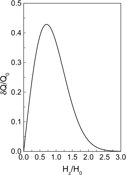
Figure 2: The behavior of the induced effective charge $\delta Q/Q_{0}$ in applied magnetic field $H_{z}/H_{0}$, according to Eq.(21).

For small applied fields ($z\ll 1$), the induced polarization $P_{x}(H_{z})\approx\alpha_{0}H_{z}$, where $\alpha_{0}=e\tau dJ/\hbar H_{0}$ is the so-called linear magnetoelectric coefficient [35]. However, as we mentioned in the very beginning, to correctly describe any induced effects in very small external fields, both Josephson junction pinning and ”self-field” effects have to be taken into account. At the same time, in view of Eq.(16) the induced polarization is related to the corresponding change of the effective charge $\delta Q\equiv(1/d)\sum_{i}<q_{i}x_{i}>$ in applied magnetic field as follows

$$\delta Q(H_{z})=\frac{P_{x}(H_{z})}{d}=Q_{0}G(H_{z}/H_{0}),$$ (21)

where $Q_{0}=e\tau J/\hbar$.

It is of interest also to consider the related field behavior of the effective flux capacitance $\delta C\equiv\tau d\delta Q(H_{z})/d\Phi$ which in view of Eq.(21) reads

$$\delta C(H_{z})=C_{0}\left(1-2\frac{H_{z}^{2}}{H_{0}^{2}}\right)e^{-H_{z}^{2}/H_{0}^{2}},$$ (22)

where $\Phi=SH_{z}$, and $C_{0}=\tau Q_{0}/\Phi_{0}$. Figure 2 shows the behavior of the induced effective charge $\delta Q/Q_{0}$ in applied magnetic field $H_{z}/H_{0}$. As is seen, at $H_{z}/H_{0}\approx 0.8$ the effective charge reaches its maximum (while the capacitance changes its sign at this field), suggesting a significant redistribution of the junction charge balance in a model system under the influence of an applied magnetic field, near the Josephson critical field $H_{0}$. Note that a somewhat similar behavior of the magnetic field induced charge (and related capacitance) has been observed in 2D electron systems [36].

Taking $\tau=10^{-10}s$ for the Josephson relaxation time (which is related to the Josephson plasma frequency, $\omega_{p}\simeq\tau^{-1}$, known to be the characteristic frequency of the system for $E_{C}\ll J$ regime, with $E_{C}$ being the Coulomb grain’s charge energy; typically $\omega_{p}=10^{9}-10^{11}Hz$) and $J/k_{B}=90K$ for a zero-temperature Josephson energy in $YBCO$ ceramics, we arrive at the following estimates of the effective charge $Q_{0}\approx 10^{-16}C$, flux capacitance $C_{0}\approx 10^{-11}F$, the equivalent current $I_{0}\sim Q_{0}/\tau\approx 10^{-6}A$, and voltage $V_{0}\sim Q_{0}/C_{0}\approx 10^{-5}V$. We note that the above set of estimates fall into the range of parameters used in typical experiments to study the charging effects both in single JJs (with the working frequency from RF range of $\omega\simeq 10GHz$ used to stimulate the system [13]) and JJAs [37] suggesting thus quite an optimistic possibility to observe the above-predicted field induced effects experimentally, using a specially prepared system of arrays of superconducting grains.

4. STRESS INDUCED PARAMAGNETIC MEISSNER EFFECT

The possibility to observe tangible piezoeffects in mechanically loaded grain boundary Josephson junctions (GBJJs) is based on the fact that under plastic deformation, grain boundaries (GBs) (which are the natural sources of weak links in HTCS), move rather rapidly via the movement of the grain boundary dislocations (GBDs) comprising these GBs [38-40]. Using the above evidence, in Ref.8 a piezophase response of a single GBJJ (created by GBDs strain field $\epsilon_{d}$ acting as an insulating barrier of thickness $l$ and height $U$ in a $SIS$-type junction with the Josephson energy $J\propto e^{-l\sqrt{U}}$) to an applied stress was considered. To understand how piezoeffects manifest themselves through GBJJs, let us invoke an analogy with the so-called thermophase effect [6,7] (a quantum mechanical alternative for the conventional thermoelectric effect) in JJs. In essence, the thermophase effect assumes a direct coupling between an applied temperature drop $\Delta T$ and the resulting phase difference $\Delta\phi$ through a JJ. When a rather small temperature gradient is applied to a JJ, an entropy-carrying normal current $I_{n}=L_{n}\Delta T$ (where $L_{n}$ is the thermoelectric coefficient) is generated through such a junction. To satisfy the constraint dictated by the Meissner effect, the resulting supercurrent $I_{s}=I_{c}\sin[\Delta\phi]$ (with $I_{c}=2eJ/h$ being the Josephson critical current) develops a phase difference through a weak link. The normal current is locally canceled by a counterflow of supercurrent, so that the total current through the junction $I=I_{n}+I_{s}=0$. As a result, supercurrent $I_{c}\sin[\Delta\phi]=-I_{n}=-L_{n}\Delta T$ generates a nonzero phase difference leading to the linear thermophase effect [6,7] $\Delta\phi\simeq-L_{tp}\Delta T$ with $L_{tp}=L_{n}/I_{c}(T)$.

By analogy, we can introduce a piezophase effect (as a quantum alternative for the conventional piezoelectric effect) through a JJ [8,16]. Indeed, a linear conventional piezoelectric effect relates induced polarization $P_{n}$ to an applied strain $\epsilon$ as [35] $P_{n}=d_{n}\epsilon$, where $d_{n}$ is the piezoelectric coefficient. The corresponding normal piezocurrent density is $j_{n}=dP_{n}/dt=d_{n}\dot{\epsilon}$ where $\dot{\epsilon}(\sigma)$ is a rate of plastic deformation which depends on the number of GBDs of density $\rho$ and a mean dislocation rate $v_{d}$ as follows [41] $\dot{\epsilon}(\sigma)=b\rho v_{d}(\sigma)$ (where $b$ is the absolute value of the appropriate Burgers vector). In turn, $v_{d}(\sigma)\simeq v_{0}(\sigma/\sigma_{m})$. To meet the requirements imposed by the Meissner effect, in response to the induced normal piezocurrent, the corresponding Josephson supercurrent of density $j_{s}=dP_{s}/dt=j_{c}\sin[\Delta\phi]$ should emerge within the contact. Here $P_{s}=-2enb$ is the Cooper pair’s induced polarization with $n$ the pair number density, and $j_{c}=2ebJ/\hbar V$ is the critical current density. The neutrality conditions ($j_{n}+j_{s}=0$ and $P_{n}+P_{s}=const$) will lead then to the linear piezophase effect $\Delta\phi\simeq-d_{pp}\dot{\epsilon}(\sigma)$ (with $d_{pp}=d_{n}/j_{c}$ being the piezophase coefficient) and the concomitant change of the pair number density under an applied strain, viz., $\Delta n(\epsilon)=d_{pn}\epsilon$ with $d_{pn}=d_{n}/2eb$.

To adequately describe magnetic properties of a granular superconductor, we again employ a model of random three-dimensional (3D) overdamped Josephson junction array which is based on the familiar tunneling Hamiltonian given by Eq.(1) (see Section 2). According to the above-discussed scenario, under mechanical loading the superconducting phase difference will acquire an additional contribution $\delta\phi_{i,j}(\sigma)=-B\vec{\sigma}\cdot\vec{r}_{i,j}$, where $B=d_{n}\dot{\epsilon}_{0}/\sigma_{m}j_{c}b$ with $\dot{\epsilon}_{0}=b\rho v_{0}$ being the maximum deformation rate and the other parameters defined earlier. If, in addition to the external loading, the network of superconducting grains is under the influence of an applied frustrating magnetic field $\vec{H}$, the total phase difference through the contact reads

$$\phi_{i,j}(\vec{H},\vec{\sigma})=\phi^{0}_{i,j}+\frac{\pi}{\Phi_{0}}(\vec{r}_{i,j}\wedge\vec{R}_{i,j})\cdot\vec{H}-B\vec{\sigma}\cdot\vec{r}_{i,j}$$ (23)

Once again, to neglect the influence of the self-field effects in a real material, the corresponding Josephson penetration length $\lambda_{J}$ must be much larger than the junction (or grain) size. Likewise, to ensure the uniformity of the applied stress $\sigma$, we also assume that $d\ll\lambda_{\sigma}$, where $\lambda_{\sigma}$ is a characteristic length over which $\sigma$ is kept homogeneous.

When the Josephson supercurrent $I_{i,j}^{s}=I_{c}\sin\phi_{i,j}$ circulates around a set of grains, it induces a random magnetic moment $\vec{\mu}_{s}$ of the Josephson network which results in the stress induced net magnetization (Cf. Eq.(8))

$$\vec{M}_{s}(\vec{H},\vec{\sigma})\equiv<\vec{\mu}_{s}>=\int\limits_{0}^{\infty}d\vec{r}_{i,j}d\vec{R}_{i,j}f(\vec{r}_{i,j},\vec{R}_{i,j})\vec{\mu}_{s}$$ (24)

To capture the very essence of the superconducting piezomagnetic effect, in what follows we assume for simplicity that an unloaded sample does not possess any spontaneous magnetization at zero magnetic field (that is $M_{s}(0,0)=0$) and that its Meissner response to a small applied field $H$ is purely diamagnetic (that is $M_{s}(H,0)\simeq-H$). According to Eq.(23), this condition implies $\phi^{0}_{i,j}=2\pi m$ for the initial phase difference with $m=0,\pm 1,\pm 2,..$.

Taking the applied stress along the $x$-axis, $\vec{\sigma}=(\sigma,0,0)$, normally to the applied magnetic field $\vec{H}=(0,0,H)$, and assuming an exponential distribution law for the distance between grains, $f_{r}(\vec{r})=f(x)f(y)f(z)$ with $f(x_{j})=(1/d)e^{-x_{j}/d}$ (see Section 2 for detailes), we get finally

$$M_{s}(H,\sigma)=-M_{0}(\sigma)\frac{H_{tot}(H,\sigma)/H_{0}}{[1+H^{2}_{tot}(H,\sigma)/H^{2}_{0}]^{2}},$$ (25)

for the induced transverse magnetization, where $H_{tot}(H,\sigma)=H-H^{*}(\sigma)$ is the total magnetic field with $H^{*}(\sigma)=[\sigma/\sigma_{0}(\sigma)]H_{0}$ being a stress-induced contribution. Here, $M_{0}(\sigma)=I_{c}(\sigma)SN/V$ with $S=\pi dD$ being a projected area around the JJ, $H_{0}=\Phi_{0}/S$, and $\sigma_{0}(\sigma)=\sigma_{m}[j_{c}(\sigma)/j_{d}](b/d)$ with $j_{d}=d_{n}\dot{\epsilon}_{0}$ and $\dot{\epsilon}_{0}=b\rho v_{0}$ being the maximum values of the dislocation current density and the plastic deformation rate, respectively.

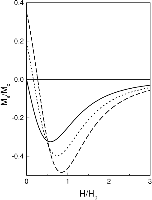
Figure 3: The reduced magnetization $M_{s}/M_{c}$ as a function of the reduced applied magnetic field $H/H_{0}$, according to Eq.(25) for different values of reduced applied stress: $\sigma/\sigma_{c}=0$ (solid line), $\sigma/\sigma_{c}=0.01$ (dotted line), and $\sigma/\sigma_{c}=0.05$ (dashed line).

According to the recent experiments [43], the tunneling dominated critical current $I_{c}$ (and its density $j_{c}$) in HTCS ceramics was found to exponentially increase under compressive stress, viz. $I_{c}(\sigma)=I_{c}(0)e^{\beta\sigma}$ with $\beta\simeq 1/\sigma_{m}$. Specifically, the critical current at $\sigma=9kbar$ was found to be three times higher its value at $\sigma=1.5kbar$, clearly indicating a weak-links-mediated origin of the phenomenon (in the best defect-free thin films this ratio is controlled by the stress induced modifications of the carrier number density and practically never exceeds a few percents [42]). Strictly speaking, the critical current will also change (decrease) with applied magnetic field. However, for the fields under discussion (see below) in the first approximation this effect can be neglected. In view of Eq.(25), dependence of $I_{c}$ on $\sigma$ will lead to a rather strong piezomagnetic effects. Indeed, Fig.3 shows changes of the initial stress-free diamagnetic magnetization $M_{s}/M_{c}$ (solid line) under an applied stress $\sigma/\sigma_{c}$. Here $M_{c}\equiv M_{0}(0)$ and $\sigma_{c}\equiv\sigma_{0}(0)$ (see below for estimates). As we see, already relatively small values of an applied stress render a low field Meissner phase strongly paramagnetic (dotted and dashed lines) simultaneously increasing the maximum of the magnetization and shifting it towards higher magnetic fields. According to Eq.(25), the initially diamagnetic Meissner effect turns paramagnetic as soon as the piezomagnetic contribution $H^{*}(\sigma)$ exceeds an applied magnetic field $H$. To see whether this can actually happen in a real material, let us estimate a magnitude of the piezomagnetic field $H^{*}$. Typically, for HTCS ceramics $S\approx 10\mu m^{2}$, leading to $H_{0}\simeq 1G$. To estimate the needed value of the dislocation current density $j_{d}$, we turn to the available experimental data. According to Ref.39, a rather strong polarization under compressive pressure $\sigma/\sigma_{m}\simeq 0.1$ was observed in $YBCO$ ceramic samples at $T=77K$ yielding $d_{n}=10^{2}C/m^{2}$ for the piezoelectric coefficient. Usually, for GBJJs $\dot{\epsilon}_{0}\simeq 10^{-2}s^{-1}$, and $b\simeq 10nm$ leading to $j_{d}=d_{n}\dot{\epsilon}_{0}\simeq 1A/m^{2}$ for the maximum dislocation current density. Using the typical values of the critical current density $j_{c}(\sigma)=10^{4}A/m^{2}$ (found [43] for $\sigma/\sigma_{m}\simeq 0.1$) and grain size $d\simeq 1\mu m$, we arrive at the following estimate of the piezomagnetic field $H^{*}\simeq 10^{-2}H_{0}$. Thus, the predicted stress induced paramagnetic Meissner effect should be observable for applied magnetic fields $H\simeq 10^{-2}H_{0}\simeq 0.01G$ which correspond to the region where the original PME was first registered [1-3]. In turn, the piezoelectric coefficient $d_{n}$ is related to a charge $Q$ in the GBJJ as [44] $d_{n}=(Q/S)(d/b)^{2}$. Given the above-obtained estimates, we get $Q\simeq 10^{-13}C$ for an effective charge accumulated by the GBs. Notice that the above values of the aplied stress $\sigma$ and the resulting effective charge $Q$ correspond (via the so-called electroplastic effect [44]) to an equivalent applied electric field $E=b^{2}\sigma/Q\simeq 10^{7}V/m$ at which rather pronounced electric-field induced effects in HTCS have been recently observed [17-21].

Besides, according to Ref.43 the Josephson projected area $S$ slightly decreases under pressure thus leading to some increase of the characteristic field $H_{0}=\Phi_{0}/S$. In view of Eq.(25), it means that a smaller compression stress is needed to actually reverse the sign of the induced magnetization $M_{s}$. Furthermore, if an unloaded granular superconductor already exhibits the PME, due to the orbital currents induced spontaneous magnetization resulting from an initial phase difference $\phi^{0}_{i,j}=2\pi r$ in Eq.(23) with fractional $r$ (in particular, $r=1/2$ corresponds to the so-called [2,3,21] $\pi$-type state), then according to our scenario this effect will either be further enhanced by applying a compression (with $\sigma>0$) or will disappear under a strong enough extension (with $\sigma<0$). Given the markedly different mechanisms and scales of stress induced changes in defect-free thin films [42] and weak-links-ridden ceramics [43], it should be possible to experimentally register the suggested here piezophase effects.

ACKNOWLEDGMENTS

This work was conceived and partially done during my stay at the Universidade Federal de São Carlos (Brazil) where it was funded by the Brazilian Agency FAPESP (Projeto 2000/04187-8). I thank Wilson Ortiz and Fernando Araujo-Moreira for hospitality and stimulating discussions on the subject. I am also indebted to Anant Narlikar for his invitation to make this contribution for the current volume of the Studies.

References

- [1] W. Braunisch et al., Phys. Rev. Lett. 68 (1992) 1908.
- [2] F.V. Kusmartsev, Phys. Rev. Lett. 69 (1992) 2268.
- [3] M. Sigrist and T.M. Rice, Rev. Mod. Phys. 67 (1995) 503.
- [4] F. M. Araujo-Moreira et al., Phys. Rev. Lett. 78 (1997) 4625.
- [5] P. Barbara, F. M. Araujo-Moreira, A. B. Cawthorne, and C. J. Lobb, Phys. Rev. B 60 (1999) 7489.
- [6] G.D. Guttman et al., Phys. Rev. B 55 (1997) 12691.
- [7] S. Sergeenkov, JETP Lett. 67 (1998) 680.
- [8] S. Sergeenkov, J. Phys.: Cond. Mat. 10 (1998) L265.
- [9] L. Legrand et al., Europhys. Lett. 34 (1996) 287.
- [10] W. A. C. Passos, F. M. Araujo-Moreira and W. A. Ortiz, J. Appl. Phys. 87 (2000) 5555.
- [11] M. Iansity et al., Phys. Rev. Lett. 60 (1988) 2414.
- [12] D.B. Haviland et al., Z. Phys. B 85 (1991) 339.
- [13] H.S.J. van der Zant, Physica B 222 (1996) 344.
- [14] S. Sergeenkov, J. Phys. I France 7 (1997) 1175.
- [15] S. Sergeenkov and J. José, Europhys. Lett. 43 (1998) 469.
- [16] S. Sergeenkov, JETP Lett. 70 (1999) 36.
- [17] B.I. Smirnov et al., Phys. Solid State 34 (1992) 1331.
- [18] B.I. Smirnov et al., Phys. Solid State 35 (1993) 1118.
- [19] T.S. Orlova and B.I. Smirnov, Supercond. Sci. Techn. 7 (1994) 899.
- [20] A.L. Rakhmanov and A.V. Rozhkov, Physica C 267 (1996) 233.
- [21] D. Dominguez, C. Wiecko and J. José, Phys. Rev. Lett. 83 (1999) 4164.
- [22] See, e.g., Magnetoelectric Interaction Phenomena in Crystals, ed. by A.J. Freeman and H. Schmid (Gordon and Breach, New York, 1975).
- [23] L.S. Levitov et al., Sov. Phys. JETP 61 (1985) 133.
- [24] V.M. Edelstein, Phys. Rev. Lett. 75 (1995) 2004.
- [25] I.E. Dzyaloshinskii, Sov. Phys. JETP 37 (1959) 881; T. Moriya, Phys. Rev. 120 (1960) 91.
- [26] C. Ebner and D. Stroud, Phys. Rev. B 31 (1985) 165.
- [27] J. Choi and J. José, Phys. Rev. Lett. 62 (1989) 320. See also, G. Blatter et al., Rev. Mod. Phys. 66 (1994) 1125.
- [28] T.K. Kopeć and J.V. José, Phys. Rev. B 52 (1995) 16140.
- [29] M. Tinkham, Introduction to Superconductivity, (McGraw-Hill, New York, 1996).
- [30] C. Lebeau et al., Europhys. Lett. 1 (1986) 313.
- [31] D. Dominguez and J.V. José, Phys. Rev. B 53 (1996) 11692.
- [32] B. Mühlschlegel and D.L. Mills, Phys. Rev. B 29 (1984) 159.
- [33] A. Barone and G. Paterno, Physics and Applications of the Josephson Effect (Wiley, New York, 1982).
- [34] A. Majhofer, Physica B 222 (1996) 273.
- [35] L.D. Landau and E.M. Lifshitz, Electrodynamics of Continuous Media (Pergamon Press, Oxford, 1984).
- [36] W. Chen et al., Phys. Rev. Lett. 73 (1994) 146.
- [37] C. Lebeau et al., Physica B 152 (1988) 100.
- [38] E.Z. Meilikhov and R.M. Farzetdinova, JETP Lett. 65 (1997) 32.
- [39] T.J. Kim et al., J. Alloys Compd. 211/212 (1994) 318.
- [40] V.N. Kovalyova et al., Sov. J. Low Temp. Phys. 17 (1991) 46.
- [41] A.H. Cottrell, Dislocations and Flow in Crystals (Clarendon Press, Oxford, 1953).
- [42] G.L. Belenky et al., Phys. Rev. B 44 (1991) 10117.
- [43] A.I. D’yachenko et al., Physica C 251 (1995) 207.
- [44] Yu.A. Osip’yan et al., Adv. Phys. 35 (1986) 115.