Emptiness Formation Probability for the One-Dimensional Isotropic ${XY}$ Model

Abstract

We study a correlation function for the one-dimensional isotropic ${XY}$ model (${XX0}$ model), which is called the Emptiness Formation Probability (EFP). It is the probability of the formation of a ferromagnetic string in the anti-ferromagnetic ground state. Using the expression of the EFP as a Toeplitz determinant, we discuss its asymptotic behaviors. We also compare the analytical results with numerical calculations as the density-matrix renormalization group and the quantum Monte-Carlo method.

1 Introduction

Recently there have been a lot of progresses for the calculation of correlation functions for the one-dimensional ${XXZ}$ model [1, 2, 3, 4, 5, 6, 7, 8],

$$\mathcal{H}=J\sum^{N}_{j=1}\left\{S^{x}_{j}S^{x}_{j+1}+S^{y}_{j}S^{y}_{j+1}+\Delta S^{z}_{j}S^{z}_{j+1}\right\}-2h\sum^{N}_{j=1}S^{z}_{j},$$ (1)

which is exactly solved by the Bethe ansatz method [9]. Among various correlation functions, the so called emptiness formation probability (EFP) ${P(n)}$

$$P(n)=\langle\prod^{n}_{j=1}(S^{z}_{j}+\frac{1}{2})\rangle,$$ (2)

is the most fundamental one [3].

Concerning the asymptotic behaviours of ${P(n)}$ for ${|\Delta|\leq 1}$, the following properties have been discussed:
(1) ${P(n)}$ decays like a Gaussian at zero temperature [5].
(2) ${P(n)}$ decays exponentially at finite temperature [8].
In this paper, we shall confirm these properties for the isotropic ${XY}$ model (${\Delta=0}$) [10, 11] in detail. Actually, based on the representation of ${P(n)}$ as a Fredholm determinant [5], (c.f. eq. (21)), the property (1) has been established for generic ${|\Delta|\leq 1}$ to some extent .

For the special case, ${\Delta=0}$, we will show in this paper that ${P(n)}$ can be alternatively represented by a Toeplitz determinant. The representation by Toeplitz determinant is very powerful to give us more information on the properties of ${P(n)}$. Actually there are theorems known for the asymptotics of the Toeplitz determinants, which directly establish properties (1) and (2). They also give us the complete forms of the asymptotic behaviours including the prefactor.

On the other hand, we can calculate ${P(n)}$ for small ${n}$ by other numerical methods. In this paper we employ the density-matrix renormalization group (DMRG) method for zero temperature case and the quantum Monte-Carlo (QMC) method for finite temperature case. The numerical data calculated by the DMRG and the QMC agree satisfactorily with the analytical ones. We believe the method and the results presented in this paper will afford a good foundation when we investigate the EFP for other models.

The plan of the paper is as follows. In §2, we derive the representation of ${P(n)}$ by Toeplitz determinant. The asymptotic form of ${P(n)}$ is obtained from Widom’s theorem. In §3, we demonstrate a numerical simulation of ${P(n)}$ by DMRG and compare with the analytical calculation. In §4, the EFP at the finite temperature is studied. This time the asymptotic function is obtained from Szegö’s theorem. It is compared with the numerical calculations by QMC in §5. The last section is devoted to summary and discussions.

2 EFP at Zero Temperature

The Hamiltonian of the isotropic ${XY}$ model is defined by the special case of (1) with ${\Delta=0}$, i.e.,

$$\mathcal{H}=J\sum^{N}_{j=1}\left\{S^{x}_{j}S^{x}_{j+1}+S^{y}_{j}S^{y}_{j+1}\right\}-2h\sum^{N}_{j=1}S^{z}_{j},$$ (3)

where $S^{\alpha}_{j}$ are the spin 1/2 operators

$$[S^{\alpha}_{k},S^{\beta}_{l}]=i\delta_{kl}\epsilon_{\alpha\beta\gamma}S^{\gamma}_{k},$$ (4)

and are represented by the Pauli matrices $\sigma^{\alpha}_{j}$ as

$$S^{\alpha}_{j}=\frac{1}{2}\sigma^{\alpha}_{j},$$

$$\sigma^{x}_{j}=\left[\begin{array}[]{@{\,}cc@{\,}}0&1\\ 1&0\\ \end{array}\right],\sigma^{y}_{j}=\left[\begin{array}[]{@{\,}cc@{\,}}0&-\textrm{i}\\ \textrm{i}&0\\ \end{array}\right],\sigma^{z}_{j}=\left[\begin{array}[]{@{\,}cc@{\,}}1&0\\ 0&-1\\ \end{array}\right].$$ (11)

In the Hamiltonian (3), we assume the periodic boundary condition (PBC),

$$S^{\alpha}_{N+1}\equiv S^{\alpha}_{1}.$$ (12)

We also introduce ${S^{\pm}_{k}\equiv S^{x}_{k}\pm iS^{y}_{k}}$ for later convenience. The EFP at zero temperature is defined by

$$P(n)=\langle GS|\prod^{n}_{j=1}(S^{z}_{j}+\frac{1}{2})|GS\rangle,$$ (13)

which represents the probability of the formation of a ferromagnetic string with a length $n$ in the anti-ferromagnetic ground state ${|GS\rangle}$.

The Hamiltonian (3) can be diagonalized by means of the Jordan-Wigner transformation [10],

$$S^{-}_{k} =\prod^{k-1}_{j=1}(1-2c_{j}^{\dagger}c_{j})c_{k}^{\dagger},$$

$$S^{+}_{k} =\prod^{k-1}_{j=1}(1-2c_{j}^{\dagger}c_{j})c_{k},$$ (14)

where $c^{\dagger}_{k},c_{k}$ are the fermion creation and annihilation operators, respectively. In fact, the Hamiltonian (3) is transformed to a spinless fermion model as

$$\mathcal{H} =-\frac{J}{2}\sum^{N-1}_{j=1}(c^{\dagger}_{j+1}c_{j}+c^{\dagger}_{j}c_{j+1})-hN+2h\sum^{N}_{j=1}c^{\dagger}_{j}c_{j}$$

$$\ \ \ \ +\frac{J}{2}\left\{\displaystyle{\prod^{N}_{k=1}}(1-2c^{\dagger}_{k}c_{k})\right\}(c^{\dagger}_{1}c_{N}+c^{\dagger}_{N}c_{1}).$$ (15)

We can diagonalize the Hamiltonian (15) by means of the Fourier transformation. In the thermodynamic limit ${(N\rightarrow\infty)}$, the ground state energy is given by

$$e=-h+{\frac{1}{2\pi}}\int^{k_{\textrm{F}}}_{-k_{\textrm{F}}}(2h-J\cos q)\textrm{d}q,$$ (16)

where the Fermi point $k_{\rm F}$ is determined by

$$k_{\rm F}=\cos^{-1}(2h/J).$$ (17)

Note that $k_{\textrm{F}}$ goes to zero as ${h\rightarrow h_{\textrm{c}}\equiv J/2}$. The EFP (13) can be calculated by use of the Fermion operators as

$$P(n) =\langle\prod^{n}_{j=1}c_{j}c^{\dagger}_{j}\rangle$$

$$=\det[\langle c_{l}c^{\dagger}_{m}\rangle]^{n}_{l,m=1}$$

$$=\det\left[\frac{1}{2\pi}\int^{2\pi-k_{\textrm{F}}}_{k_{\textrm{F}}}{\rm e}^{\textrm{i}(l-m)q}\textrm{d}q\right]^{n}_{l,m=1},$$ (18)

where we have used Wick’s theorem. A kind of the determinant like eq. (18) is referred to as a Toeplitz determinant.

It is known that the transverse correlation function ${\langle S_{r}^{x}S_{0}^{x}\rangle}$ for the ${XY}$ model is also written as a slightly different Toeplitz determinant [10]. It decays algebraically as ${(r\rightarrow\infty)}$,

$$\langle S_{r}^{x}S_{0}^{x}\rangle\sim 1/\sqrt{r}.$$ (19)

Similarly, the longitudinal correlation function decays algebraically

$$\langle\langle S_{r}^{z}S_{0}^{z}\rangle\rangle\equiv\langle S_{r}^{z}S_{0}^{z}\rangle-\langle S_{r}^{z}\rangle\langle S_{0}^{z}\rangle\sim 1/r^{2}.$$ (20)

For further results on these correlation functions, see the refs. 10,12–20.

As we shall show below, the asymptotic behavior of ${P(n)}$ is remarkably different from the two point correlation functions above.

We remark that there are two other representations for ${P(n)}$.
(1) Fredholm determinant representation [18, 4]:

$$P(n)=\det\left[I-K_{n}\right],$$ (21)

where $K_{n}$ is a linear integral operator acting on functions on interval $[-k_{\textrm{F}},k_{\textrm{F}}]$ with a kernel

$$K_{n}(p,q) =\frac{1}{2\pi}\sum_{j=0}^{n-1}\textrm{e}^{\textrm{i}(p-q)j}$$

$$=\frac{\textrm{e}^{\frac{(n-1)(p-q)}{2}\textrm{i}}}{2\pi}\frac{\sin\frac{n}{2}(p-q)}{\sin\frac{1}{2}(p-q)}.$$ (22)

Or equivalently,

$$P(n) =\sum_{j=0}^{n}\frac{(-1)^{j}}{j!}\int_{-k_{\textrm{F}}}^{k_{\textrm{F}}}{\rm d}q_{1}\cdots\int_{-k_{\textrm{F}}}^{k_{\textrm{F}}}\textrm{d}q_{j}\det\left[K_{n}(q_{l},q_{m})\right]_{l,m=1}^{j}$$

$$=\frac{1}{n!}\int_{k_{\textrm{F}}}^{2\pi-k_{\textrm{F}}}\textrm{d}q_{1}\cdots\int_{k_{\textrm{F}}}^{2\pi-k_{\textrm{F}}}\textrm{d}q_{n}\det\left[K_{n}(q_{l},q_{m})\right]_{l,m=1}^{n}.$$ (23)

For the derivation of the equalities above, we refer to ref. 24.

Note that the kernel ${K_{n}(p,q)}$ (22) can be replaced by

$$\frac{\sin\frac{n}{2}(p-q)}{2\pi\sin\frac{1}{2}(p-q)},$$ (24)

due to a property of the determinant [18].

(2) Multiple integral representation [6, 25]:

$$P(n) =(-1)^{\frac{n(n-1)}{2}}2^{\frac{n(n+1)}{2}}\int_{R}\frac{\textrm{d}\lambda_{1}}{2\pi}\cdots\int_{R}\frac{\textrm{d}\lambda_{n}}{2\pi}\prod_{a>b}\frac{\sinh 2(\lambda_{a}-\lambda_{b})}{\sinh(\lambda_{a}-\lambda_{b}-\frac{\pi}{2}i)}$$

$$\ \ \ \ \ \ \ \ \ \ \ \ \ \ \ \ \times\prod_{j=1}^{n}\frac{\sinh^{j-1}(\lambda_{j}-\frac{\pi}{4}i)\sinh^{n-j}(\lambda_{j}+\frac{\pi}{4}i)}{\cosh^{n}2\lambda_{j}}.$$ (25)

Here the integration range ${R}$ is defined by

$$\int_{R}\textrm{d}\lambda\equiv\left\{\begin{array}[]{ll}\displaystyle\int_{-\Lambda}^{\Lambda}{\rm d}\lambda&\mbox{for ${k_{\textrm{F}}\geq\frac{\pi}{2}}$}\\[8.61108pt] \displaystyle\left(\int_{-\infty}^{\infty}+\int_{-\infty}^{-\Lambda}+\int_{\Lambda}^{\infty}\right){\rm d}\lambda&\mbox{for ${k_{\textrm{F}}<\frac{\pi}{2}}$}\end{array}\right.$$ (26)

where the endpoint ${\Lambda}$ is related to ${k_{\textrm{F}}}$ through

$$\textrm{e}^{-2\Lambda}=-\textrm{i}\frac{\textrm{e}^{\textrm{i}k_{\textrm{F}}}-\textrm{i}}{\textrm{e}^{\textrm{i}k_{\textrm{F}}}+\textrm{i}}.$$ (27)

The integral representation (25) was first obtained in ref. 25, in the case of ${\Lambda=\infty}$. Recently it was confirmed and generalized to finite ${\Lambda}$ case in ref. 6.

We can show that eqs. (18), (21) and (25), are all equivalent [21, 24, 25]. For the readers’ convenience, we give some brief proofs in Appendix A and Appendix B.

Note that the Fredholm determinant representation (1) and the multiple integral representation (2) do exist for the general ${XXZ}$ model (1) [4, 5, 2, 25, 6], while the Toeplitz determinant (18) is very special to the ${XY}$ model. However, in the following, we discuss the asymptotic properties of $P(n)$ for the isotropic ${XY}$ model (3) based on the representation (18).

Let us first assume that ${h}$ takes some moderate value, $|h|<h_{\rm c}$. Then from Widom’s theorem [27] for the Toeplitz determinant (18), we immediately obtain

$$\ln P(n)=n^{2}\ln\cos\frac{k_{\rm F}}{2}-\frac{1}{4}\ln(n\sin{\frac{k_{\rm F}}{2}})+\frac{1}{12}\ln 2+3\zeta^{{}^{\prime}}(-1)+o(1),$$ (28)

i.e.,

$$P(n)\simeq 2^{\frac{1}{12}}{\rm e}^{3\zeta^{{}^{\prime}}(-1)}\left(\sin\frac{k_{\textrm{F}}}{2}\right)^{-\frac{1}{4}}n^{-1/4}\left(\cos\frac{k_{\textrm{F}}}{2}\right)^{n^{2}},\ \ \ \ (n\rightarrow\infty),$$ (29)

where $\zeta(x)$ is Riemann’s zeta function. We note that ${\zeta^{{}^{\prime}}(-1)=-0.165421\cdots}$ and

$$2^{\frac{1}{12}}\textrm{e}^{3\zeta^{{}^{\prime}}(-1)}=0.645002\cdots.$$ (30)

In terms of the external magnetic field $h$, the formula (29) can be expressed as

$$P(n)\simeq 2^{\frac{1}{12}}\textrm{e}^{3\zeta^{{}^{\prime}}(-1)}\left(\frac{1-2h/J}{2}\right)^{-\frac{1}{8}}n^{-\frac{1}{4}}\left(\frac{1+2h/J}{2}\right)^{\frac{n^{2}}{2}},\ \ \ \ (n\rightarrow\infty).$$ (31)

Thus $P(n)$ for the isotropic ${XY}$ model (3) decays like a Gaussian. The speed of Gaussian decay as well as the prefactor depends on the magnetic field $h$. The fact that ${P(n)}$ shows Gaussian decay has been established in ref. 5, 23 and 26. Especially we remark that the dependence on the magnetic field ${h}$ in the part of Gaussian decay was already obtained in ref. 5. Their method is based on the solution of the Riemann-Hilbert problem associated with the Fredholm determinant (21). However, the prefactor and the part ${n^{-1/4}}$ have not been obtained from the Riemann-Hilbert approach yet.

We observe that the prefactor of (28) diverges as ${h}$ gets closer to the critical value, i.e., ${h\rightarrow h_{\rm c}=J/2}$. There the asymptotic formula (31) may not be adequate. For this region, as ${k_{\rm F}}$ is very small, we can expand the determinant (18) with respect to ${k_{\rm F}}$. Actually we can easily obtain the expansion,

$$P(n) =1-\frac{k_{\textrm{F}}}{\pi}n+\frac{k_{\textrm{F}}^{4}}{36\pi^{2}}n^{2}(n^{2}-1)-\frac{k_{\textrm{F}}^{6}}{675\pi^{2}}n^{2}(n^{2}-1)(n^{2}-\frac{3}{2})+\cdots,$$ (32)

which may be useful to study the critical behaviors of ${P(n)}$ near ${h=h_{\rm c}}$.

In Fig. 1, we plot ${P(n)}$ and the corresponding asymptotic function (29) for several magnetizations ${m\equiv\langle S_{j}^{z}\rangle}$. Here note that ${m}$ is connected to ${k_{\rm F}}$ as

$$m=\frac{1}{2}-\frac{k_{\textrm{F}}}{\pi}.$$ (33)

The readers will observe ${P(n)}$ is well fitted by the asymptotic function (29).

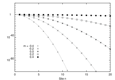
Figure 1: $P(n)$ at zero temperature.

We would like to remark that the Toeplitz determinant (18) appears in relation to the level spacing distribution of the random matrix theory [21]. More precisely, the function ${A_{2}(\alpha)}$ for Dyson’s circular ensemble of ${n\times n}$ unitary matrices, is identical to eq. (18) with the correspondence ${\alpha=k_{\textrm{F}}}$. Here ${A_{2}(\alpha)}$ means the probability that an interval (of the unit circle) of length ${2\alpha}$ contains no eigenvalues. The function ${A_{2}(\alpha)}$ has been studied profoundly in the context of the random matrix theory. Then we can translate all the results obtained for ${A_{2}(\alpha)}$ to ${P(n)}$. For example, it is recently shown that ${A_{2}(\alpha)}$ satisfies an integrable non-linear differential equation, which is equivalent to Painlevé VI equation [22, 23]. Hence our ${P(n)}$ also satisfies the Painlevé VI equation [23].

3 Numerical Simulation by DMRG Method

In this section, we perform numerical simulation so as to confirm the validity of the asymptotic form (29). We employed the density-matrix renormalization group (DMRG) here [28, 29].The method has an advantage in that it allows us to treat large system sizes. Our algorithm here is standard, and its detail would be found in literatures; we refer the readers to ref. 30. Hence, below, we will outline some technical points that are relevant to our simulation precision: We implemented the infinite-system method, which is adequate to study the ground-state properties in thermodynamic limit. We have repeated hundreds of renormalizations. At each renormalization, we remained, at most, two-hundred relevant states (bases) for a block; namely, in conventional terminology, we set $m=200$. The density-matrix eigenvalue $\{w_{\alpha}\}$ of each remained base indicates its significance (weight). We found $w_{\alpha}>10^{-10}$. That is, weights of discarded states are no more than $w_{\alpha}\sim 10^{-10}$.

However, there are some subtleties in the DMRG calculation when ${S=1/2}$ as in our present case. The number of spins consisting each block increases by one after another through each renormalization. The problem is that the structure of the Hilbert space changes significantly according to the situations whether block contains even number of spins or odd number of spins. (Note that for ${S=1}$, such difficulty does not arise.) Therefore simulation data alternate in turn through renormalizations, even though we repeat hundreds of renormalizations. In this respect, the translational symmetry is broken intrinsically in the scheme. In other words, edge effect remains through renormalizations. In fact, as for ${P(2)}$, for instance, the digit of order ${10^{-3}}$ alternates. We coped with the difficulty by averaging the data over two successive renormalizations. Then we could achieve the precision of ${10^{-4}}$ for ${P(2)}$. The precision of data would be improved further if we use a certain careful extrapolation. However, in the following, we shall show that our data reproduces the analytical results rather satisfactorily.

In Fig. 2, we plot the data for ${P(n)}$ obtained by the DMRG simulation. The dotted lines represent the asymptotic functions (29). For the positive magnetization ${m=0,0.2,0.4}$, we also list the explicit numerical data in Table 1–3. We find our numerical data by DMRG agree well with the analytical ones in §2.

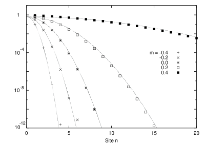
Figure 2: Numerical calculation of $P(n)$ by DMRG.

Table 1: ${P(n)}$ for ${\langle S_{j}^{z}\rangle=0}$

${n}$	DMRG	exact values
1	${0.500}$	${0.5}$
2	${1.486\times 10^{-1}}$	${1.487\times 10^{-1}}$
3	${2.367\times 10^{-2}}$	${2.368\times 10^{-2}}$
4	${1.940\times 10^{-3}}$	${1.945\times 10^{-3}}$
5	${8.096\times 10^{-5}}$	${8.126\times 10^{-5}}$
6	${1.699\times 10^{-6}}$	${1.715\times 10^{-6}}$
7	${1.795\times 10^{-8}}$	${1.823\times 10^{-8}}$
8	${9.559\times 10^{-11}}$	${9.740\times 10^{-11}}$
9	${4.578\times 10^{-13}}$	${2.612\times 10^{-13}}$
10	${2.442\times 10^{-14}}$	${3.514\times 10^{-14}}$

Table 2: ${P(n)}$ for ${\langle S_{j}^{z}\rangle=0.2}$

$n$	DMRG	exact values
1	${0.699}$	${0.7}$
2	${4.219\times 10^{-1}}$	${4.237\times 10^{-1}}$
3	${2.123\times 10^{-2}}$	${2.140\times 10^{-2}}$
4	${8.717\times 10^{-2}}$	${8.840\times 10^{-2}}$
5	${2.890\times 10^{-2}}$	${2.950\times 10^{-2}}$
6	${7.673\times 10^{-3}}$	${7.907\times 10^{-3}}$
7	${1.628\times 10^{-3}}$	${1.695\times 10^{-3}}$
8	${2.750\times 10^{-4}}$	${2.902\times 10^{-4}}$
9	${3.713\times 10^{-5}}$	${3.960\times 10^{-5}}$
10	${4.004\times 10^{-6}}$	${4.304\times 10^{-6}}$

Table 3: ${P(n)}$ for ${\langle S_{j}^{z}\rangle=0.4}$

$n$	DMRG	exact values
1	${0.899}$	${0.9}$
2	${7.984\times 10^{-1}}$	${8.003\times 10^{-1}}$
3	${6.993\times 10^{-1}}$	${7.019\times 10^{-1}}$
4	${6.028\times 10^{-1}}$	${6.061\times 10^{-1}}$
5	${5.103\times 10^{-1}}$	${5.146\times 10^{-1}}$
6	${4.238\times 10^{-1}}$	${4.290\times 10^{-1}}$
7	${3.455\times 10^{-1}}$	${3.508\times 10^{-1}}$
8	${2.758\times 10^{-1}}$	${2.811\times 10^{-1}}$
9	${2.161\times 10^{-1}}$	${2.206\times 10^{-1}}$
10	${1.655\times 10^{-1}}$	${1.695\times 10^{-1}}$

We see that for very small $P(n)<10^{-12}$, simulation data start to deviate widely from the analytical ones. This may be simply due to the numerical round-off error; note that (double precision) real number is stored as sixteen digits in computer and the data of very small ${P(n)}$ are not reliable in principle. For large $h(\sim 0.4)$, $P(n)$ decays slowly and our data yield results reliable even for very large distances. Actually, from Table 3, we see that the deviation is less than few percents even for ${n=10}$.

From the numerical data of ${P(n)}$ for small ${n}$, we can estimate a plausible asymptotic form,

$$P(n)\simeq{\rm const}\times a^{-n^{2}}\ n^{\alpha}.$$ (34)

In fact, by fitting successive three data for ${P(n)}$ in the form (34), we get the approximate values for ${{\rm const},a}$ and ${\alpha}$. We show an example in Table 4, where each parameter is obtained from ${P(k),P(k+1)}$ and ${P(k+2)}$.

Table 4: Estimation of the fitting parameters by DMRG: ${\langle S_{j}^{z}\rangle=0}$

${k}$	${a}$	const	${\alpha}$
1	${1.415}$	${0.707}$	${-0.247}$
2	${1.415}$	${0.709}$	${-0.251}$
3	${1.414}$	${0.719}$	${-0.271}$
4	${1.416}$	${0.673}$	${-0.204}$
5	${1.415}$	${0.723}$	${-0.265}$

The exact parameters in the asymptotic function (29) are

$$a=1.414,\ \ {\rm const}=0.703,\ \ \alpha=-0.25.$$ (35)

Thus we could perfectly estimate the speed of Gaussian decay, ${a}$. We also got reasonable approximate values for the prefactor and the exponent ${\alpha}$. From these results, we can insist that the DMRG method provides a powerful means to study the EFP at zero temperature for the 1D spin systems.

4 EFP at Finite Temperature

At finite temperature $(T>0)$, the EFP is defined by

$$P(n)=\langle\prod^{n}_{j=1}(S^{z}_{j}+\frac{1}{2})\rangle_{T}\equiv\frac{{\rm Tr}(\textrm{e}^{-\mathcal{H}/T}\prod^{n}_{j=1}(S^{z}_{j}+\frac{1}{2}))}{{\rm Tr}(\textrm{e}^{-\mathcal{H}/T})}.$$ (36)

For the isotropic ${XY}$ model, we can represent eq. (36) in terms of a Toeplitz determinant by use of the finite temperature version of Wick’s theorem (Bloch-de Dominicis theorem) as follows.

$$P(n) =\det\left[\langle c_{l}c_{m}^{\dagger}\rangle_{T}\right]_{l,m=1}^{n}$$

$$=\det\left[\frac{1}{2\pi}\int_{0}^{2\pi}\textrm{e}^{\textrm{i}(l-m)q}\rho(q)\textrm{d}q\right]_{l,m=1}^{n},$$ (37)

where

$$\rho(q) =\frac{1}{1+\textrm{e}^{-\varepsilon(q)/T}}=1-\frac{1}{1+\textrm{e}^{\varepsilon(q)/T}},$$

$$\varepsilon(q) =2h-J\cos q.$$ (38)

Note that ${1/(1+\textrm{e}^{\varepsilon(q)/T})}$ is nothing but the Fermi distribution function. Compared with the zero temperature case, we can see that the integration range in each matrix element is replaced as

$$\int_{k_{\textrm{F}}}^{2\pi-k_{\textrm{F}}}\textrm{d}q\longrightarrow\int_{0}^{2\pi}\rho(q)\textrm{d}q.$$ (39)

However, the asymptotic behavior of eq. (37) is quite different from eq. (18) . In fact, this time we can apply Szegö’s theorem to the Toeplitz determinant like (37) (see Chapter 10 in ref. 31). The theorem tells us

$$\ln P(n)=n\rho_{0}+\sum^{\infty}_{k=1}k\rho_{k}\rho_{-k}+o(1),$$ (40)

where

$$\ln\rho(q)=\sum^{\infty}_{k=-\infty}\rho_{k}\textrm{e}^{\textrm{i}kq}.$$ (41)

In particular, we have

$$\rho_{0}=-{\frac{1}{2\pi}}\int_{0}^{2\pi}\ln(1+{\rm e}^{-\varepsilon(q)/T}){\rm d}q,$$ (42)

Now recall that the free energy per site for the isotropic ${XY}$ model is given by [10, 11]

$$f(T,h)=-h-\frac{T}{2\pi}\int_{0}^{2\pi}\ln(1+{\rm e}^{-\varepsilon(q)/T}){\rm}{\rm d}q.$$ (43)

Then we can conclude that $P(n)$ decays exponentially at finite temperature as

$$P(n)\simeq c(T,h)\exp\left(-\frac{n}{\xi}\right).$$ (44)

where the inverse of the correlation length ${\xi^{-1}}$ and the prefactor $c(T,h)$ are given by

$$\xi^{-1} =-\frac{f(T,h)+h}{T}$$

$$=\frac{1}{2\pi}\int_{0}^{2\pi}\ln\left[1+\exp\left(\frac{J\cos q-2h}{T}\right)\right]\textrm{d}q,$$ (45)

$$c(T,h) =\exp\left(\sum^{\infty}_{k=1}k\rho_{k}\rho_{-k}\right),$$ (46)

respectively. Note a formula

$$\sum^{\infty}_{k=1}k\rho_{k}\rho_{-k}=\frac{1}{8}\int_{0}^{2\pi}\frac{{\rm d}q}{2\pi}\int_{0}^{2\pi}\frac{{\rm d}\tilde{q}}{2\pi}\left(\frac{\ln\rho(q)-\ln\rho(\tilde{q})}{\sin\frac{1}{2}(q-\tilde{q})}\right)^{2},$$ (47)

which can be found on page 112 of ref. 32. It is useful for numerical evaluation of ${c(T,h)}$ (46).

At finite temperature, it is known that the correlation functions such as ${\langle S_{r}^{x}S_{0}^{x}\rangle}$ and ${\langle\langle S_{r}^{z}S_{0}^{z}\rangle\rangle}$ also decay exponentially. The correlation lengths of these correlation functions have been calculated analytically in refs. 15 and 33–35 as

$$\xi_{xx}^{-1} =\frac{1}{2\pi}\int_{0}^{2\pi}\textrm{d}q\ln\left(\coth\left|\frac{J\cos q-2h}{2T}\right|\right),$$ (48)

$$\xi_{zz}^{-1} =\sinh^{-1}\left(\frac{\pi T-2ih}{J}\right)+\sinh^{-1}\left(\frac{\pi T+2ih}{J}\right).$$ (49)

In Fig. 3 and Fig. 4, we show some plots of ${P(n)}$ calculated from eq. (37) for ${T=0.05}$ and ${T=1}$. The dotted lines are the asymptotic functions (44).

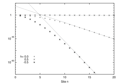
Figure 3: $P(n)$ at a low temperature : ${J=1,T=0.05}$.

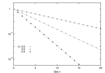
Figure 4: $P(n)$ at a high temperature : ${J=1,T=1}$.

We observe the asymptotic behaviors of ${P(n)}$ are actually described by eq. (44). Particularly in the high temperature case (${T=1}$), even ${P(n)}$ for small ${n}$ are well fitted by eq. (44). At low temperature (${T=0.05}$), ${P(n)}$ deviates from eq. (44) for small ${n}$. At this region, ${P(n)}$ may behave more like Gaussian as in the zero temperature case.

It is known that, when ${|h|<h_{\textrm{c}}}$, the low temperature expansion of the free-energy (43) is given by [11, 36],

$$f(T,h)=e-\frac{\pi T^{2}}{6v_{\rm s}}+O(T^{3}),$$ (50)

where ${e}$ is the ground state energy (16) and ${v_{\rm s}}$ is the velocity of a low energy excitation

$$v_{\rm s}=J\cos^{-1}\left(2h/J\right).$$ (51)

From eq. (50), we can obtain the low temperature expansion of ${\xi^{-1}}$ as

$$\xi^{-1} =\frac{1}{\pi T}\left\{J\sin\left[\cos^{-1}\left(2h/J\right)\right]-2h\cos^{-1}\left(2h/J\right)\right\}$$

$$\ \ \ \ +\frac{\pi T}{6J\cos^{-1}(2h/J)}+O(T^{2}).$$ (52)

Thus we find the inverse of the correlation length ${\xi^{-1}}$ diverges when ${T\rightarrow 0}$ as long as ${|h|<h_{\rm c}}$. That is, the correlation length ${\xi}$ approaches to zero in the low temperature limit, which signals a crossover of the exponential decay to a stronger (Gaussian) decay in §2 and §3. This is in a remarkable contrast to the low temperature behaviors of ${\xi_{xx}}$ (48) and ${\xi_{zz}}$ (49). They behave as ${\sim 1/T}$ in the low temperature limit, which results from a crossover to a weaker (algebraic) decay.

When the magnetic field is critical, i.e., ${h=\pm h_{\textrm{c}}}$  ${(h_{\textrm{c}}=J/2)}$, the low temperature expansion of the free-energy takes a differnt form [36],

$$f(T,h)=-h_{\textrm{c}}-\frac{1}{\sqrt{2\pi J}}\zeta\left(\frac{3}{2}\right)\left(1-\frac{1}{\sqrt{2}}\right)T^{3/2}+O(T^{2}).$$ (53)

Accordingly, the low temperature behavior of ${\xi^{-1}}$ at ${h=\pm h_{\textrm{c}}}$ is given by

$$\xi^{-1}=\left\{\begin{array}[]{l}\displaystyle\frac{1}{\sqrt{2\pi J}}\zeta\left(\frac{3}{2}\right)\left(1-\frac{1}{\sqrt{2}}\right)\sqrt{T}+O(T),\ \ \ \ \ \ \ \ \ \ \ \ \mbox{(for ${h=h_{\textrm{c}}}$)}\\[8.61108pt] \displaystyle\frac{2h_{\textrm{c}}}{T}+\frac{1}{\sqrt{2\pi J}}\zeta\left(\frac{3}{2}\right)\left(1-\frac{1}{\sqrt{2}}\right)\sqrt{T}+O(T),\ \ \ \ \mbox{(for ${h=-h_{\textrm{c}}}$)}\end{array}\right.$$ (54)

respectively. Thus we find particularly that ${\xi^{-1}}$ goes to zero as ${\sim\sqrt{T}}$ when ${h=h_{\textrm{c}}}$.

In Fig. 5, we plot the temperature dependences of ${\xi^{-1}}$. We observe the low temperature behaviors of ${\xi^{-1}}$ are actually described by eqs. (52) and (54).

Figure 5: Temperature dependence of ${\xi^{-1}}$ : ${J=1}$.

We also plot the prefactor ${c(T,h)}$ in Fig. 6. When ${h<h_{\textrm{c}}}$, the prefactor ${c(T,h)}$ diverges in the low temperature limit.

Figure 6: Temperature dependence of the prefactor ${c(T,h)}$ : ${J=1}$.

In the high temperature limit (${T\rightarrow\infty}$), we have

$$P(n)\rightarrow\left(\frac{1}{2}\right)^{n},$$ (55)

since

$$\xi^{-1}\rightarrow\ln(2),\ \ c(T,h)\rightarrow 1.$$ (56)

Alternatively, we can regard the magnetic field $h$ as a function of the temperature and fix the magnetization

$$m\equiv\langle S_{j}^{z}\rangle_{T}=\frac{1}{2}-\frac{1}{2\pi}\int_{0}^{2\pi}\textrm{d}q\frac{1}{1+\textrm{e}^{\varepsilon(q)/T}}.$$ (57)

In this case, since

$$\ln\rho(q)\rightarrow\frac{1}{1+\textrm{e}^{-2h/T}},\ \ \ \ \ \ \ \ m\rightarrow\frac{1}{2}-\frac{1}{1+\textrm{e}^{2h/T}},$$ (58)

we have

$$P(n)\rightarrow\left(\frac{1}{2}+m\right)^{n}=P(1)^{n},$$ (59)

as ${T\rightarrow\infty}$.

5 Numerical Simulation by QMC Method

In this section, we perform numerical simulations in order to confirm the analytical theory for ${P(n)}$ at finite temperatures described in the previous section. Here we employ the quantum Monte-Carlo (QMC) method [37]. For finite-temperature calculations, the QMC method is particularly of use. In fact, recently, there have been proposed a number of substantial improvements: In ref. 38, an algorithm involving infinite Trotter-decomposition number is presented; that is, the continuous-time algorithm. Employing this algorithm, the authors had demonstrated that the simulation result is completely free from the Trotter-decomposition error. In addition, with the use of global update algorithm postulated in refs. 39–41, the auto-correlation time is reduced to considerable extent so that we can avoid wasting Monte-Carlo steps (the so-called critical slowing down). Hence, Monte-Carlo simulation combined with these techniques would be promising for studying long-range form of $P(n)$ precisely.

We treated systems with size $N=128$, and imposed the periodic boundary condition. We performed five-million Monte-Carlo steps initiated by 0.5 million steps for reaching thermal equilibrium. ${P(n)}$ is measured and averaged over the five-million Monte-Carlo steps. The results for ${T=1}$ are plotted in Fig. 7. We see that the data are governed by the analytical asymptotic function postulated in §4 (shown by the dotted lines). We have performed the simulations for several other temperatures and magnetic fields. The obtained data exhibit good coincidence with the analytical ones unless the temperature is exceedingly low ${(T\leq 0.1)}$. In this way we could confirm the validity of the asymptotic formula (44) numerically at least for moderate temperatures. Unfortunately when the temperature is very low, the QMC simulation does not work very efficiently so that we could not reproduce the data such as at ${T=0.05}$ yet.

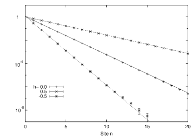
Figure 7: $P(n)$ calculated by QMC method : ${J=1,T=1}$.

6 Summary and Discussion

In this paper we have studied ${P(n)}$ for the isotropic ${XY}$ model in detail. Especially we have obtained the expression of ${P(n)}$ in terms of Toeplitz determinant. On the basis of the expression, we could calculate the exact values of ${P(n)}$ for small ${n}$ and also get the asymptotic expression as ${n\rightarrow\infty}$.

At zero temperature, Widom’s theorem for Toeplitz determinant gives us the complete asymptotic function directly. It agrees and completes the previous known results on the asymptotics of ${P(n)}$. The asymptotic form of ${P(n)}$ is given by

$$P(n)\sim a^{-n^{2}}\ n^{\alpha},$$ (60)

with

$$a=1.4142,\ \ \ \ \alpha=-0.25,$$ (61)

for zero magnetic field. For small ${n}$, we have also calculated ${P(n)}$ by means of the DMRG method. In general, DMRG is not so efficient to investigate system at criticality such as eq. (3), because any correlation evaluated with the method, in principle, decays exponentially at large distances [42]. However, we have found that as for $P(n)$, which decays like a Gaussian, the method yields precise result as well as correct asymptotic form. We could also estimate the speed of Gaussian decay ${a}$, etc., numerically. The method will be applied to other models in the forthcoming papers.

We could obtain ${P(n)}$ in terms of Toeplitz determinant also at finite temperature. This time from Szegö’s theorem, we have shown analytically that ${P(n)}$ decays exponentially as ${n\rightarrow\infty}$,

$$P(n)\sim\exp{\frac{(f+h)n}{T}}.$$ (62)

We have confirmed this formula independently by means of the QMC method.

It is Boos and Korepin [8] who first obtained the asymptotic formula (62) for any ${\Delta}$ when ${h=0}$. They derived the formula from an observation of the definition of the thermodynamics, which can be generalized to the finite ${h}$ case straightforwardly [43]. In the forthcoming papers, we will plan to confirm (62) for other models by use of the QMC method. It may be also possible to discuss ${P(n)}$ at finite temperature from the point of view of the quantum transfer matrix method [33, 34, 35, 44, 45, 46, 47, 48, 49].

Appendix A Equivalence of eq. (21) and eq. (18)

Here we will show (23), i.e.,

$$\frac{1}{n!}\int_{k_{\textrm{F}}}^{2\pi-k_{\textrm{F}}}\frac{\textrm{d}q_{1}}{2\pi}\cdots\int_{k_{\textrm{F}}}^{2\pi-k_{\textrm{F}}}\frac{\textrm{d}q_{n}}{2\pi}\det\bigg{[}\sum_{j=0}^{n-1}\textrm{e}^{\textrm{i}(q_{l}-q_{m})j}\bigg{]}_{l,m=1}^{n},$$ (63)

is transformed to the Toeplitz determinant (18). Actually from

$$\det\Bigg{[}\sum_{j=0}^{n-1}\textrm{e}^{\textrm{i}(q_{l}-q_{m})j}\Bigg{]}_{l,m=1}^{n} =\det\left[{\rm e}^{\textrm{i}q_{l}j}\right]\det\left[{\rm e}^{-\textrm{i}q_{m}k}\right]$$

$$=\det\left[\sum_{l=1}^{n}\textrm{e}^{\textrm{i}(j-k)q_{l}}\right]_{j,k=0}^{n-1},$$ (64)

we can see (63) is equal to

$$\int_{k_{\textrm{F}}}^{2\pi-k_{\textrm{F}}}\frac{\textrm{d}q_{1}}{2\pi}\cdots\int_{k_{\textrm{F}}}^{2\pi-k_{\textrm{F}}}\frac{\textrm{d}q_{n}}{2\pi}\det\left[\textrm{e}^{\textrm{i}(j-k)q_{k}}\right]_{j,k=0}^{n-1}=\det\bigg{[}\int_{k_{\textrm{F}}}^{2\pi-k_{\textrm{F}}}\frac{\textrm{d}q}{2\pi}\textrm{e}^{\textrm{i}(j-k)q}\bigg{]}_{j,k=0}^{n-1}.$$ (65)

The last expression is identical to the Toeplitz determinant (18).

Appendix B Equivalence of eq. (25) and eq. (18)

We will show the multiple integral formula (25) is reduced to the Toeplitz determinant (18). Here we assume ${k_{\rm F}\geq\dfrac{\pi}{2}}$ for simplicity.

From the relation

$$\sinh(x-\dfrac{\pi}{2}\textrm{i})=-\textrm{i}\cosh x,$$ (66)

the integral formula (25) is written as

$$P(n) =(-\textrm{i})^{\frac{n(n-1)}{2}}2^{\frac{n(n+1)}{2}}\int_{-\Lambda}^{\Lambda}\frac{\textrm{d}{\lambda_{1}}}{2\pi}\cdots\int_{-\Lambda}^{\Lambda}\frac{\textrm{d}{\lambda_{n}}}{2\pi}$$

$$\ \ \ \ \times\prod_{a>b}2\sinh(\lambda_{a}-\lambda_{b})\prod_{j=1}^{n}\frac{\sinh^{j-1}(\lambda_{j}-\frac{\pi}{4}\textrm{i})\sinh^{n-j}(\lambda_{j}+\frac{\pi}{4}\textrm{i})}{\cosh^{n}2\lambda_{j}}.$$ (67)

Furthermore by using the relations

$$\prod_{a>b}2\sinh(\lambda_{a}-\lambda_{b}) =\prod_{a>b}\left(\textrm{e}^{\lambda_{a}-\lambda_{b}}-\textrm{e}^{\lambda_{b}-\lambda_{a}}\right)$$

$$=\det\left[\textrm{e}^{(2k-n-1)\lambda_{j}}\right]_{j,k=1}^{n},$$ (68)

and

$$\cosh 2\lambda_{j}=2\sinh\left(\lambda_{j}-\frac{\pi}{4}\textrm{i}\right)\sinh\left(\lambda_{j}+\frac{\pi}{4}\textrm{i}\right),$$ (69)

we can find that eq. (67) is represented by the determinant,

$$P(n)=(-\textrm{i})^{\frac{n(n-1)}{2}}2^{\frac{n(n+1)}{2}}\det[I_{jk}]_{j,k=1}^{n}$$ (70)

where

$$I_{jk}=\int_{-\Lambda}^{\Lambda}\frac{{\rm d}\lambda}{2\pi}\frac{2\textrm{e}^{2k\lambda}}{(\textrm{e}^{2\lambda}-\textrm{i})^{n-j-1}({\rm e}^{2\lambda}+\textrm{i})^{j}}.$$ (71)

Now we introduce a change of integration variable from ${\lambda}$ to ${x}$ defined by

$$\textrm{e}^{2\lambda}=-\textrm{i}\frac{\textrm{e}^{\textrm{i}x}-\textrm{i}}{\textrm{e}^{\textrm{i}x}+\textrm{i}}.$$ (72)

Then after some simple calculations, one can find the determinant representation (67) becomes

$$P(n)={(-2\textrm{i})}^{\frac{n(1-n)}{2}}\det[\tilde{I}_{jk}]_{j,k=1}^{n},$$ (73)

where

$$\tilde{I}_{jk}=\int_{k_{\rm F}}^{2\pi-k_{\rm F}}\frac{{\rm d}x}{2\pi}({\rm e}^{\textrm{i}x}+\textrm{i})^{n-k}({\rm e}^{\textrm{i}x}-\textrm{i})^{k-1}\textrm{e}^{\textrm{i}(j-n)x}.$$ (74)

Recall that the relation between ${\Lambda}$ and ${k_{\textrm{F}}}$ is given in eq. (27),

$$\textrm{e}^{-2\Lambda}=-\textrm{i}\frac{\textrm{e}^{\textrm{i}k_{\textrm{F}}}-\textrm{i}}{\textrm{e}^{\textrm{i}k_{\textrm{F}}}+\textrm{i}}.$$ (75)

Below we will show eq. (73) is identical to eq. (18). First we subtract the ${(n-1)}$-th column from the ${n}$-th column. Then the integrand of the ${n}$-th column can be replaced as

$$(\textrm{e}^{\textrm{i}x}-\textrm{i})^{n-1}\textrm{e}^{\textrm{i}(j-n)x}\rightarrow-2i(\textrm{e}^{\textrm{i}x}-\textrm{i})^{n-2}{\rm e}^{\textrm{i}(j-n)x}.$$ (76)

Similarly, we can subtract the ${(k-1)}$-th column from the ${k}$-th column subsequently until ${k=2}$. This procedure allows us to replace of the matrix elements for ${k\geq 2}$ as ,

$$\tilde{I}_{jk}\rightarrow-2\textrm{i}\int_{k_{\textrm{F}}}^{2\pi-k_{\textrm{F}}}\frac{\textrm{d}x}{2\pi}(\textrm{e}^{\textrm{i}x}+\textrm{i})^{n-k}(\textrm{e}^{\textrm{i}x}-\textrm{i})^{k-2}\textrm{e}^{\textrm{i}(j-n)x}.$$ (77)

The above transformation yields a factor ${(-2\textrm{i})^{n-1}}$, which cancels parts of the prefactor (73).

Next we apply the same transformation to the ${n}$-th column again and subsequently to the ${k}$-th column down to ${k=3}$. This procedure reduces the order of the factor $(\textrm{e}^{\textrm{i}x}-\textrm{i})$ in the integrand by 1 and at the same time generates a factor ${(-2\textrm{i})^{n-2}}$. Repeating the similar procedure, we finally arrive at

$$P(n)=\det\left[\int_{k_{\textrm{F}}}^{2\pi-k_{\textrm{F}}}\frac{\textrm{d}x}{2\pi}(\textrm{e}^{\textrm{i}x}+\textrm{i})^{n-k}\textrm{e}^{\textrm{i}(j-n)x}\right]_{j,k=1}^{n}.$$ (78)

Expanding ${(\textrm{e}^{\textrm{i}x}+\textrm{i})^{n-k}}$ with respect to ${\textrm{e}^{\textrm{i}x}}$, we can further simplify eq. (78) as

$$P(n) =\det\left[\int_{k_{\textrm{F}}}^{2\pi-k_{\textrm{F}}}\frac{\textrm{d}x}{2\pi}\textrm{e}^{\textrm{i}(n-k)x}\textrm{e}^{\textrm{i}(j-n)x}\right]_{j,k=1}^{n},$$

$$=\det\left[\int_{k_{\textrm{F}}}^{2\pi-k_{\textrm{F}}}\frac{\textrm{d}x}{2\pi}\textrm{e}^{\textrm{i}(j-k)x}\right]_{j,k=1}^{n}.$$ (79)

The last expression is nothing but the Toeplitz determinant (18).

References

- [1] V. E. Korepin, A. G. Izergin and N.M. Bogoliubov: Quantum Inverse Scattering Method and Correlation Functions (Cambridge University Press, Cambridge, 1993).
- [2] M. Jimbo and T. Miwa: Algebraic analysis of solvable lattice models (AMS, 1995).
- [3] V. E. Korepin, A. G. Izergin, F. H. L. Essler, D. B. Uglov: Phys. Lett. A 190 (1994) 182.
- [4] F. H. L. Essler, H. Frahm, A. G. Izergin and V. E. Korepin: Commun. Math. Phys. 174 (1995) 191.
- [5] F. H. L. Essler, H. Frahm, A. R. Its, V. E. Korepin: Nucl Phys B 446 (1995) 448.
- [6] N. Kitanine, J. M. Maillet, V. Terras: Nucl. Phys. B 567 (2000) 554.
- [7] A. V. Razmov and Yu. G. Stroganov: cond-mat/0012141, cond-mat/0102247.
- [8] H. E. Boos and V. E. Korepin: hep-th/0104088, hep-th/0105144.
- [9] M. Takahashi: Thermodynamics of One-Dimensional Solvable Models (Cambridge University Press, Cambridge, 1999).
- [10] E. H. Lieb, T. Schultz and D. Mattis: A. Phys. (N.Y.) 16 (1961) 417.
- [11] S. Katsura: Phys. Rev. 127 (1962) 1508.
- [12] T. Niemeijer: Physica 36 (1967) 377.
- [13] B. M. McCoy: Phys. Rev. 173 (1968) 531.
- [14] S. Katsura, T. Horiguchi and M. Suzuki: Physica 46 (1970) 67.
- [15] E. Barouch and B. M. McCoy: Phys. Rev. A 3 (1971) 786, 2137.
- [16] H. G. Vaidya and C. A. Tracy: Physica. 92A (1978) 1.
- [17] T. Tonegawa: Solid State Commun. 40 (1981) 983.
- [18] F. Colomo, A. G. Izergin, V. E. Korepin and V. Tognetti: Phys. Lett. A 169 (1992) 243.
- [19] A. R. Its, A. G. Izergin, V. E. Korepin and N. A. Slavnov: Phys. Rev. Lett. 70 (1993) 1704.
- [20] J. Stolze, A. Nöppert and G. Müller: Phys. Rev. B 52 (1995) 4319.
- [21] M. L. Mehta: Random Matrices, Second Edition, (Academic Press, 1991).
- [22] C. A. Tracy and H. Widom: Comm. Math. Phys. 163 (1994) 33.
- [23] P. A. Deift, A. R. Its and X. Zhou: Ann. Math. 146 (1997) 149.
- [24] P. Deift: Orthogonal Polynomials and Random Matrices: Riemann-Hilbert Approach (AMS, 2000).
- [25] M. Jimbo and T. Miwa: J. Phys. A 29 (1996) 2923.
- [26] Y. Fujii: J. Phys. Soc. Jpn. 69 (2000) 3143.
- [27] H. Widom: Indiana Univ. Math. J. 21 (1971) 277.
- [28] S. R. White: Phys. Rev. Lett. 69, (1992) 2863.
- [29] S. R. White: Phys. Rev. B 48, (1993) 10345.
- [30] Density-Matrix Renormalization — A New Numerical Method in Physics, ed. I. Peschel, X. Wang, M. Kaulke and K. Hallberg (Springer-Verlag, Berlin, Heidelberg, 1999).
- [31] T. T. Wu and B. M. McCoy: The two-dimensional Ising model (Harvard University Press, Cambride, 1973).
- [32] M. L. Mehta: Matrix Theory (Editions de Physique, Orsay, France, 1989).
- [33] M. Inoue and M. Suzuki: Prog. Theor. Phys. 79 (1988) 645.
- [34] M. Takahashi: Phys. Rev. B 44, (1991) 12382.
- [35] A. Kuniba, A. Sakai and J. Suzuki: Nucl. Phys. B 525, (1998) 597.
- [36] M. Takahashi: Prog. Theor. Phys. 50 (1973) 1519.
- [37] M. Suzuki: Prog. Theor. Phys. 56 (1976) 1454.
- [38] B. B. Beard and U.-J. Wiese: Phys. Rev. Lett. 77 (1996) 5130.
- [39] H. G. Evertz, G. Lana and M. Marcu: Phys. Rev. Lett. 70 (1993) 875.
- [40] U.-J. Wiese and H.-P. Ying: Z. Phys. B 93 (1994) 147.
- [41] N. Kawashima and J. E. Gubernatis: Phys. Rev. Lett. 73, (1994) 1295.
- [42] S. Östlund and S. Rommer: Phys. Rev. Lett. 75 (1995) 3537.
- [43] V. E. Korepin: private communication.
- [44] M. Suzuki and M. Inoue: Prog. Theor. Phys. 78 (1987) 787.
- [45] T. Koma: Prog. Theor. Phys. 78 (1987) 1213.
- [46] T. Koma: Prog. Theor. Phys. 81 (1989) 783.
- [47] J. Suzuki, Y. Akutsu and M. Wadati: J. Phys. Soc. Jpn. 59 (1990) 2667.
- [48] M. Takahashi: Phys. Rev. B 43 (1991) 5788.
- [49] A. Klümper: Z. Phys. B 91 (1993) 507.