Didier Sornette${}^{\mbox{\ref{ess},\ref{lpec}}}$ and Kayo Ide${}^{\mbox{\ref{das}}}$

Institute of Geophysics and Planetary Physics

University of California, Los Angeles

Los Angeles, CA 90095-1567

1. Also at the Department of Earth and Space Sciences, UCLA

2. Also at the Laboratoire de Physique de la Matière Condensée, CNRS UMR 6622 and Université de Nice-Sophia Antipolis, 06108 Nice Cedex 2, France

3. Also at the Department of Atmospheric Sciences, UCLA

Abstract

We present a simple two-dimensional dynamical system reaching a singularity in finite time decorated by accelerating oscillations due to the interplay between nonlinear positive feedback and reversal in the inertia. This provides a fundamental equation for the dynamics of (1) stock market prices in the presence of nonlinear trend-followers and nonlinear value investors, (2) the world human population with a competition between a population-dependent growth rate and a nonlinear dependence on a finite carrying capacity and (3) the failure of a material subject to a time-varying stress with a competition between positive geometrical feedback on the damage variable and nonlinear healing. The rich fractal scaling properties of the dynamics are traced back to the self-similar spiral structure in phase space unfolding around an unstable spiral point at the origin.

Singularities play an important role in the physics of phase transitions as well as in signatures of positive feedbacks in dynamical systems, with examples in the Euler equations of inviscid fluids [1], in vortex collapse of systems of point vortices, in the equations of General Relativity coupled to a mass field leading to the formation of black holes [2], in models of micro-organisms aggregating to form fruiting bodies [3], in models of material failure [4], of earthquakes [5] and of stock market crashes [6].

The continuous scale invariance usually associated with a singularity can be partially broken into a weaker symmetry, called discrete scale invariance (DSI), according to which the self-similarity holds only for integer powers of a specific factor $\lambda$ [7]. The hallmark of this DSI is the transformation of the power law into an oscillatory singularity, with log-periodic oscillations decorating the overall power law acceleration towards the singularity. Such log-periodic power laws have been documented for many systems such as with a built-in geometrical hierarchy, as the result of a cascade of ultra-violet instabilities in growth processes and rupture, in deterministic dynamical systems, in response functions of spin systems with quenched disorder, in spinodal decomposition of binary mixtures in uniform shear flow, etc. (see [7, 8] and references therein).

Here, we introduce a general dynamical mechanism for a finite-time singularity with self-similar oscillatory behavior, based on the interplay between nonlinear positive feedback and reversal in the inertia:

$${dy_{1}\over dt} = y_{2}~{},$$ (1)

$${dy_{2}\over dt} = y_{2}|y_{2}|^{m-1}-\gamma y_{1}|y_{1}|^{n-1}~{}.$$ (2)

This model is motivated by and derived from the dynamics of stock market prices, of the world human population and of material failure as we shall see below (see [9] for detailed derivations). Our analysis of (1, 2) offers a fundamental understanding of the observed interplay between accelerating growth and accelerating (log-periodic) oscillations previously documented in speculative bubbles preceding large crashes [6, 14], the world human population [17, 16], and time-to-failure analysis of material rupture [4] (and references therein).

Stock market price dynamics: the heterogeneous behavior of agents has recently been shown to be a crucial ingredient to account for the complexity of financial time series (see [10] and references therein). Typically, “value investors” track the fundamental price $p_{f}$ of a given stock placing investment orders of (algebraic) size $\Omega_{\rm value}(t)$ while “technical analysts” use trend following strategies to place investment orders of size $\Omega_{\rm tech}(t)$. The balance between supply and demand determines the price variation from $p(t)$ to $p(t+\delta t)$ over the time interval $\delta t$ according to $\ln p(t+\delta t)-\ln p(t)={1\over L}[\Omega_{\rm value}(t)+\Omega_{\rm tech}(t)]$ [11] where $L>0$ is a market depth. We postulate the nonlinear dependence $\Omega_{\rm value}(t)=-c~{}\ln[p(t)/p_{f}]~{}|\ln[p(t)/p_{f}]|^{n-1}$, where $n>1$ and $c>0$ is a constant. The case $n=1$ retrieves an ingredient of previous models [11, 12]. According to textbook economics, $p_{f}$ is determined by the discounted expected future dividends whose estimation is very sensitive to the forecast of their growth rate and of the interest rate, leading to large uncertainties in $p_{f}$. As a consequence, a trader trying to track fundamental value has no incentive to react when she feels that the deviation is small since this deviation is more or less within the noise. Only when the departure of price from fundamental value becomes relatively large will the trader act. The exponent $n>1$ precisely accounts for this effect. The second class of investors follow strategies that are positively related to past price moves. This can be captured by the following contribution to the order size: $\Omega_{\rm tech}(t)=a_{1}[\ln p(t)-\ln p(t-\delta t)]+a_{2}[\ln p(t)-\ln p(t-\delta t)]|\ln p(t)-\ln p(t-\delta t)|^{m-1}$ with $a_{1}>0$ and $a_{2}>0$. The choice $m>1$ means that trend-following strategies tend to under-react for small price changes and over-react for large ones. Posing $y_{1}(t)=\ln[p(t)/p_{f}]$, we expand the equation of balance between supply and demand as a Taylor series in powers of $\delta t$ and get

$$(\delta t)^{2}{d^{2}x\over dt^{2}}=-\left[1-{a_{1}\over L}\right]~{}\delta t~{}{dx\over dt}+{a_{2}(\delta t)^{m}\over L}{dx\over dt}|{dx\over dt}|^{m-1}-{c\over L}x(t)|x(t)|^{n-1}~{}+~{}{\cal O}[(\delta t)^{3}]~{},$$ (3)

where ${\cal O}[(\delta t)^{3}]$ represents a term of the order of $(\delta t)^{3}$. This equation is a generalization of the model of Pandey and Stauffer [13], by allowing nonlinear positive feedback $m>1$ of the trend-following strategies. The theory becomes critical when the “mass” term vanishes, i.e., when $a_{1}=L$. Rescaling $t$ and $y_{1}$ by $\alpha$ and posing $y_{2}=dy_{1}/dt$ and $\gamma=\alpha^{-(n+1)}c/L(\delta t)^{2}$ where $\alpha\equiv a_{2}(\delta t)^{m-2}/L$, we obtain (1,2).

Population dynamics: the logistic equation corrects Malthus’ exponential growth model by assuming that the population $p(t)$ cannot growth beyond the earth carrying capacity $K$: ${dp\over dt}=\sigma_{0}p(t)\left[K-p(t)\right]$ where $\sigma_{0}$ controls the amplitude of the nonlinear saturation term (see [15] and references therein). However, it is now understood that $K$ is not a constant but increases with $p(t)$ due to technological progress such as the use of tools and fire, the development of agriculture, the use of fossil fuels, fertilizers etc. as well an expansion into new habitats and the removal of limiting factors by the development of vaccines, pesticides, antibiotics. If $K(t)$ grows faster than $p(t)$, then $p(t)$ explodes to infinity after a finite time creating a singularity due to the corresponding growth of the growth rate $\sigma\equiv d\ln p/dt$, leading to ${d\sigma\over dt}\propto\sigma^{2}$ [16]. We now generalize it by assuming a nonlinear saturation: ${d\sigma\over dt}=\alpha\sigma|\sigma|^{m-1}-\gamma\ln(p/K_{\infty})|\ln(p/K_{\infty})|^{n-1}$ where $\alpha$ and $\gamma>0$ measure the effect of feedback and reversal. Apart from the absolute value, the first term in the r.h.s. is the previous nonlinear growth of the growth rate. The novel second term favors a restoration of the population $p(t)$ to the asymptotic carrying capacity $K_{\infty}$. The effective cumulative growth rate $\ln(p/K_{\infty})$ is the natural variable to describe the attraction to $K_{\infty})$. The nonlinear restoring exponent $n>1$ captures the many nonlinear (often quasi-threshold) feedback mechanisms acting on population dynamics. Defining variables $(y_{1},y_{2})=(\alpha\ln(p/K_{\infty}),\sigma)$ and rescaling $t$ by $\alpha$ lead to (1,2).

Rupture of materials with competing damage and healing: a standard model of damage rupture [18] consists in a rod subjected to uniaxial tension by a constant applied axial force $P$. The undamaged cross section $A(t)$ of the rod is assumed to be a function of time but is independent of the axial coordinate. The considered viscous deformation is assumed to be isochoric: $A_{0}L_{0}=A(t)L(t)=$ constant at all times, where $L(t)$ is the length of the rod. The creep strain rate ${d\epsilon_{c}\over dt}={1\over L}{dL\over dt}=-{1\over A}{dA\over dt}$ is assumed to follow Norton’s law: ${d\epsilon_{c}\over dt}=C\sigma^{\mu}$ where $\sigma=P/A$ is the rod cross section with $C>0$ and $\mu>0$ Eliminating $d\epsilon_{c}/dt$ leads to $A^{\mu-1}dA/dt=-CP^{\mu}$, and hence ${d\sigma\over dt}=C\sigma^{\mu+1}$. Physically, this results from a geometrical feedback of the undamaged area on the stress and vice-versa.

We generalize this model by adding healing as well as a strain-dependent loading: ${d\sigma\over dt}=\alpha\sigma|\sigma|^{m-1}-\gamma\epsilon_{c}|\epsilon_{c}|^{n-1}$. The first term in the right-hand-side is identical to previous geometrical positive feedback for $m=\mu-1$. We relax this correspondence and allow $m>1$ to be arbitrary. The addition of the second term introduces the physical ingredient that damage can be reversible. Large deformations can enhance healing which increases the undamage area and thus decrease the effective stress within the material. The model is completed by using again Norton’s law but with exponent $m^{\prime}$: ${d\epsilon_{c}\over dt}=C\sigma^{m^{\prime}}$. Incorporating the constant $C$ in a redefinition of time $Ct\to t$ (with suitable redefinitions of the coefficients $\alpha/C\to\alpha$ and $\gamma/C\to\gamma$), taking $m^{\prime}=1$ and posing $(y_{1},y_{2})=(\epsilon_{c},\sigma)$, we retrieve (1,2).

Analysis of the dynamical system (1,2) for $n>1$ and $m>1$ with $\gamma\geq 0$: When only the reversal term is present (i.e., the term $y_{2}|y_{2}|^{m-1}$ is absent), (1,2) describe a non-linear oscillator with conserved Hamiltonian $H({\bf y};n,\gamma)\equiv{\gamma\over n+1}(y_{1}^{2})^{{n+1\over 2}}+{1\over 2}y_{2}^{2}$. Any trajectory is periodic along a constant $H$ with period

$$T(H;n,\gamma)=C(n)~{}\gamma^{-1\over n+1}~{}H^{{1-n\over 2(n+1)}}~{},$$ (4)

where $C(n)$ is a positive number that can be explicitly calculated [9].

When only the positive feedback is present (i.e., $\gamma=0$), (1,2) leads to a finite-time singularity. The solution ${\bf y}(t;{\bf y}_{0},t_{0})$ with initial condition ${\bf y}_{0}=(y_{10},y_{20})$ at time $t_{0}$ can be explicitly written as:

$$y_{1}(t;{\bf y}_{0},t_{0})-y_{10} = {\rm sign}[y_{20}]\frac{(m-1)^{{m-2\over m-1}}}{2-m}~{}[(t_{c}(y_{20})-t)^{{m-2\over m-1}}-(t_{c}(y_{20})-t_{0})^{{m-2\over m-1}}]~{}~{}\mbox{for $m\neq 2$};$$ (5)

$$~{}{\rm or}~{} {\rm sign}[y_{20}]~{}\log\left({t_{c}-t_{0}\over t_{c}(y_{20})-t}\right)~{}~{}\mbox{for $m=2$},$$ (6)

$$y_{2}(t;{\bf y}_{0},t_{0}) = {\rm sign}[y_{20}]~{}(m-1)^{-{1\over m-1}}~{}(t_{c}(y_{20})-t)^{-{1\over m-1}}~{},$$ (7)

where the critical time interval $t_{c}(y_{20})-t_{0}=\frac{1}{m-1}|y_{20}|^{1-m}$ depends only on $y_{20}$. As $t\to t_{c}(y_{20})$, $y_{2}$ becomes either $+\infty$ or $-\infty$ depending on the sign of $y_{20}$ for any $m>1$. For $1<m\leq 2$, it is easy to show that $|y_{1}|$ also becomes infinity as $t\to t_{c}(y_{20})$. In contrast, for $m>2$, $y_{1}$ remains finite. We thus think that $m>2$ is the relevant physical regime for the financial, population and rupture problems discussed above. From here on, our analysis focuses on $n>1$ and $m>2$.

Putting the nonlinear oscillation and positive feedback terms together, the dynamics of (1,2) is characterized in figure 1. The two special intertwined trajectories along $b^{+}$ (solid line) and $b^{-}$ (dashed line) connect the origin $(0,0)$ to $(+\infty,+\infty)$ and $(-\infty,-\infty)$, respectively, and hence divide the phase space ${\bf y}\equiv(y_{1},y_{2})$ into two distinct basins $B^{+}$ and $B^{-}$. The basin $B^{+}$ (resp. $B^{-}$) corresponds to a finite-time singularity ${\bf y}_{c}({\bf y}_{0})$ with $y_{2c}({\bf y}_{0})=+\infty$ (resp. $y_{2c}({\bf y}_{0})=-\infty$) but finite $y_{1c}({\bf y}_{0})$ at the critical time $t_{c}({\bf y}_{0})$.

Starting from ${\bf y}_{0}$ in $B^{+}$ close to the origin at $t_{0}$, a trajectory ${\bf y}(t;{\bf y}_{0},t_{0})$ spirals out with clockwise rotation and we count a turn each time it crosses the $y_{1}$-axis, i.e., $y_{1}$ changes its direction of motion ($dy_{1}/dt=0$). Deep in the spiral structure, ${\bf y}(t;{\bf y}_{0},t_{0})$ follows approximately the orbit of constant Hamiltonian $H$ defined by the nonlinear oscillator but fails to close on itself because $H$ is no longer conserved due to the positive feedback:

$${d\over dt}H({\bf y};n,m,\gamma)=|y_{2}|^{m+1}\geq 0~{}.$$ (8)

This slowly growing nonlinear oscillator defines the first dynamical regime.

Any trajectory starting in the first dynamical regime must eventually cross-over to the second one associated with a route to the singularity without any further oscillation. The second dynamical regime occurs $y_{2}$ diverges (and therefore $dy_{2}/dt$ also diverges) while $y_{1}$ remains finite on the approach to $t_{c}({\bf y}_{0})$. As a consequence, the reversal term $\gamma y_{1}|y_{1}|^{n-1}$ in $dy_{2}/dt$ (2) becomes negligible close to $t_{c}({\bf y}_{0})$ and (7) is the asymptotic solution of (1,2). Figure 2 shows a typical time series of a ${\bf y}(t;{\bf y}_{0},t_{0})$ starting from ${\bf y}_{0}$ near the origin.

In the basin $B^{+}$, the transition from the first to second dynamical regime occurs at the exit segment $\triangle e^{(+1,-0)}$ on the positive $y_{1}$-axis (figure 1) whose right and left end-points according to the forward direction of the flow are defined by the boundaries $b^{+}$ and $b^{-}$, respectively. In forward time, $\triangle e^{(+1,-0)}$ fans out rapidly over $y_{1}\in(-\infty,\infty)$ as it reaches a singularity with $y_{2}\to+\infty$ in the second dynamical regime. Note that $|y_{1}|$ can reach $\infty$ if and only if ${\bf y}_{0}$ is at an end point of $\triangle e^{(+1,-0)}$, i.e., on either $b^{+}$ or $b^{-}$. Similar results hold for the exit segment $\triangle e^{(-1,+0)}$ in $B^{-}$ but with $y_{2}\to-\infty$. In backward time, $\triangle e^{(+1,-0)}$ and $\triangle e^{(-1,+0)}$ swirl into the origin while making countable infinite many turns. These backward swirls of the exit segments completely define the first dynamical regime.

The first dynamical regime exhibits remarkable scaling properties that we quantify by the dependence on the initial condition ${\bf y}_{0}=(y_{10},0)$ on the $y_{1}$-axis of the following quantities: the number ($N_{turn})$ of turns before reaching the singularity, the exit time ($t_{e}$) to reach the exit segment into the second dynamical regime, the time interval ($\Delta t_{e}$) and the increment ($\Delta y_{1}$) in the amplitude of $y_{1}$ over one turn. Figure 3 shows log-log plots of the scaling properties measured at the $k$-th backward intersection of $b^{+}$ with the $y_{1}$-axis starting from $k=0$ at the out-most intersection (the left end-point of $\triangle e^{(-1,+0)}$ in figure 1). In order to get accurate and reliable estimations of these dependences and of the exponents defined below, we have integrated the dynamical equations using a fifth-order Runge-Kutta integration scheme with adjustable time step.

The log-log dependences shown in figure 3 qualify power laws defined by

$$N_{\rm turn} \sim y_{10}^{-a}~{},~{}~{}~{}~{}~{}~{}~{}~{}{\rm where}~{}a>0~{},$$ (9)

$$t_{e} \sim y_{10}^{-b}~{},~{}~{}~{}~{}~{}~{}~{}~{}{\rm where}~{}b>0~{},$$ (10)

$$\Delta y_{10} \sim y_{10}^{c}~{},~{}~{}~{}~{}~{}~{}~{}~{}{\rm where}~{}c>0~{},$$ (11)

$$\Delta t_{e} \sim y_{10}^{-d}~{},~{}~{}~{}~{}~{}~{}~{}~{}{\rm where}~{}d>0~{}.$$ (12)

Eliminating $y_{10}$ between (10) and (12) gives $\Delta t_{e}\sim t_{e}^{d\over b}$. Since $\Delta t_{e}$ is nothing but the difference $\Delta t_{e}=t_{e}(N_{\rm turn}+1)-t_{e}(N_{\rm turn})$, this gives the discrete difference equation ${t_{e}(N_{\rm turn}+\Delta N_{\rm turn})-t_{e}(N_{\rm turn})\over\Delta N_{\rm turn}}\propto t_{e}^{d\over b}$, where $\Delta N_{\rm turn}=N_{\rm turn}+1-N_{\rm turn}=1$. This provides a discrete difference representation of the derivative $dt_{e}/dN_{\rm turn}$ which can be integrated formally to give $N_{\rm turn}\sim t_{e}^{1-{d\over b}}$, which is valid for $d<b$. Comparing with the relation between $N_{\rm turn}$ and $t_{e}$ obtained by eliminating $y_{10}$ between (9) and (10), i.e., $N_{\rm turn}\sim t_{e}^{a\over b}$, we get the scaling relation

$$a=b-d~{}.$$ (13)

Since $a>0$, the condition $d<b$ is automatically verified.

Similarly, $\Delta y_{10}=y_{10}(N_{\rm turn}+1)-y_{10}(N_{\rm turn})\propto y_{10}^{c}$ according to definition (11). This gives the differential equation $dy_{10}/dN_{\rm turn}\sim y_{10}^{c}$, whose solution is $N_{\rm turn}\sim 1/y_{10}^{c-1}$, valid for $c>1$. Comparing with the definition (9), we get the second scaling relation

$$a=c-1~{}.$$ (14)

Since $a>0$, the condition $c>1$ is automatically satisfied.

Deep in the spiral structure depicted in figure 1, in the presence of the positive feedback term, one rotation around the origin is not exactly closed but the failure to close, which is very small especially near the origin, is quantified by $\Delta y_{10}$ shown in figure 2 which follows (11). We approximate the time $\Delta t_{e}$ needed to make one full (almost closed) rotation by the period $T(H)$ without the positive feedback term. This is essentially an adiabatic approximation in which the Hamiltonian $H$ and the period $T(H)$ are assumed to vary sufficiently slowly so that the local period of rotation follows adiabatically the variation of the Hamiltonian $H$. Putting together (4) and the fact that the amplitude of $y_{10}$ is proportional to $H^{1\over n+1}$, we get $\Delta t_{e}\sim|y_{10}|^{1-n\over 2}$, which, by comparison with (12), gives

$$d={n-1\over 2}~{}.$$ (15)

The last equation is provided by $dT/dt$, expressed as $dT/dt=(dT/dH)\times(dH/dt)$, where $dT/dH$ is obtained by differentiating (4) and $dH/dt$ is given by (8). Estimating $dT/dH$ from (4) is consistent with the above approximation in which a full rotation along the spiral takes the same time as the corresponding closed orbit in absence of the positive feedback term. Expressing $dH/dt$ using (8) involves another approximation, which is similar in spirit to a mean-field approximation corresponding to average out the effect of the positive feedback term over one full rotation. In so doing, we average out the subtle positive and negative interferences between the reversion and positive feedback terms. We replace $dT/dt$ by $d\Delta t_{e}/dt_{e}$ and obtain ${d\Delta t_{e}\over dt_{e}}\sim H^{-{3n+1\over 2(n+1)}}~{}|y_{2}|^{m+1}\sim\Delta t_{e}^{3n+1\over n-1}~{}|y_{10}|^{(n+1)(m+1)\over 2}$, where the dependence in $\Delta t_{e}$ is derived by replacing $H$ by its dependence as a function of $T$ (by inverting $T(H)$) and by identifying $T$ and $\Delta t_{c}$. We have also used $|y_{2}|\sim|y_{10}|^{n+1\over 2}$. Taking the derivative of $\Delta t_{e}\sim t_{e}^{d\over b}$ with respect to $t_{e}$ provides another estimation of ${d\Delta t_{e}\over dt_{e}}$, and replacing $\Delta t_{e}$ in the above equation by its dependence as a function of $y_{10}$ as defined by (12) gives finally:

$$a={1\over 2}(n+1)(m+1)-{1\over 2}(3n+1)~{}.$$ (16)

We find a perfect agreement between the theoretical predictions (13), (14), (15), (16) for the exponents $a,b,c,d$ defined by (9)-(12) with an estimation obtained from the direct numerical integration of the dynamical equations [9]. We have also verified the independence of the exponents $a,b,c,d$ with respect to the amplitude $\gamma$ of the reversal term.

In the oscillatory regime, the growth of the amplitude of $y_{1}(t)$ follows a power law similar to (7). We obtain it by combining some of the previous scaling laws (9-12). Indeed, taking the ratio of (11) and (12) yields $\Delta y_{1}/\Delta t_{e}\sim y_{1}^{c+d}$. Since $\Delta y_{1}$ corresponds to the growth of the local amplitude $A_{y_{1}}$ of the oscillations of $y_{1}(t)$ due to the positive feedback term over one turn of the spiral in phase space, this turn lasting $\Delta t_{e}$, we identify this scaling law with the equation for the growth rate of the amplitude $A_{y_{1}}$ of $y_{1}$ in this oscillatory regime: ${dA_{y_{1}}\over dt}\sim A_{y_{1}}^{c+d}$ whose solution is $A_{y_{1}}(t)={B\over(t^{*}-t)^{1/b}}$, where $B$ is another amplitude. This prediction is verified accurately from our direct numerical integration of the equations of motion [9]. We have used the scaling relations (13) and (14) leading to $c+d-1=b$. The time $t^{*}$ is a constant of integration such that $B/(t^{*})^{1\over b}=A_{y_{1}}(t_{0})$, which can be interpreted as an apparent or “ghost” critical time. $t^{*}$ has no reason to be equal to $t_{e}$, in particular since the extrapolation of $A_{y_{1}}(t)={B\over(t^{*}-t)^{1/b}}$ too close to $t^{*}$ would predict a divergence of $y_{1}(t)$. The dynamical origin of the difference between $t^{*}$ and $t_{c}$ comes from the fact that $t^{*}$ is determined by the oscillatory regime while $t_{c}$ is the sum of two contributions, one from the oscillatory regime and the other from the singular regime.

Combining (12) with this solution for $A_{y_{1}}(t)$ gives the time dependence of the local period $\Delta t_{e}$ of the oscillation in the oscillatory regime as $\Delta t_{e}=t_{k+1}-t_{k}\sim(t^{*}-t_{k})^{d\over b}$, where $k$ is the turn index previously used. This result generalizes the log-periodic oscillation associated with discrete scale invariance (DSI) characterized by $t_{k+1}-t_{k}\sim 1/\lambda^{k}$ (where $\lambda>1$ is a preferred scaling ratio of DSI), which is recovered in the limit $d/b\to 1^{-}$ (corresponding to ($n\to\infty,m\to 2$). The dynamical system (1,2) provides a mechanism for generalized log-periodic oscillations with, in addition, a finite number of them due to the cross-over to the non-oscillatory regime. We shall report elsewhere on tests of this theory on financial and rupture data.

Acknowledgments: This work was partially supported by ONR N00014-99-1-0020 (KI) and by NSF-DMR99-71475 and the James S. Mc Donnell Foundation 21st century scientist award/studying complex system (DS).

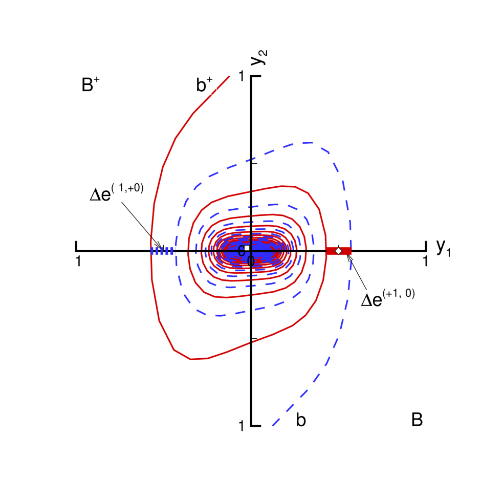
FIG. 1.: Geometry of the boundaries $b^{+}$ and $b^{-}$ as well as the basins $B^{+}$ and $B^{-}$ for $(n,m)=(3,2.5)$ and $\gamma=10$ in phase space: the exit segments $\triangle e^{(+1,-0)}\in B^{+}$ and $\triangle e^{(-1,+0)}\in B^{-}$ are thick solid and dashed lines respectively on the $y_{1}$-axis; the squares and diamonds are the initial condition and exit point of the trajectory in Figure 2.

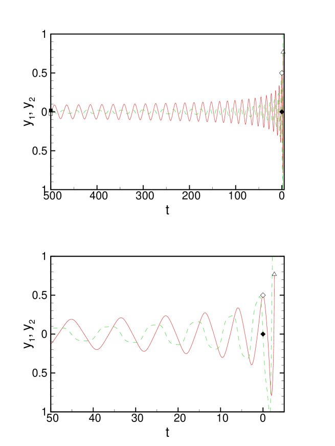
FIG. 2.: A trajectory in $B^{+}$ starting from initial condition $(-2.32878\times 10^{-2},1.71083\times 10^{-2})$ at $t=-500$, going through the exit point $(0.5,0)$ at $t=0$, to the critical point $(0.768899,+\infty)$ at $t_{c}=2.67284$: Solid and dashed lines correspond to $y_{1}$ and $y_{2}$, respectively; square, diamond and triangle are the initial condition, the point in the exit segment $\triangle e^{(+1,-0)}$, and the critical point along the trajectory with open and filled symbols corresponding to $y_{1}$ and $y_{2}$.

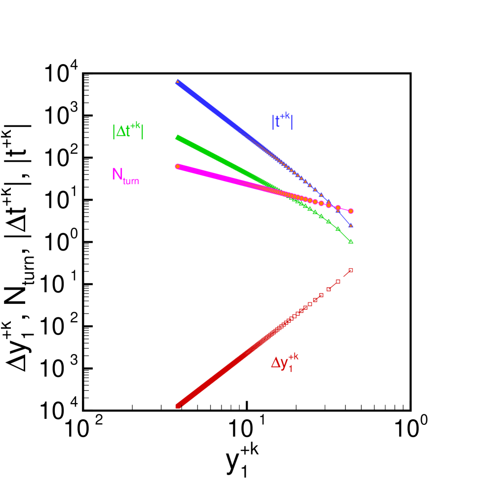
FIG. 3.: Scaling laws associated with the self-similar properties of the nonlinear oscillatory regime as a function of initial conditions at turn points for $(n,m)=(3,2.5)$ and $\gamma=10$.

REFERENCES

- [1] Pumir A. and Siggia E.D., Phys. Rev. A 45, R5351-5354 (1992).
- [2] Choptuik M.W., Prog. Theor. Phys. Suppl. 136, 353 (1999).
- [3] Rascle M. and Ziti C., J. Math. Biol. 33, 388 (1995).
- [4] Johansen, A. and D. Sornette, Eur. Phys. J. B 18, 163 (2000).
- [5] Johansen A, Saleur, H., Sornette, D., Eur. Phys. J. B 15, 551 (2000).
- [6] Johansen, A., Sornette, D. and Ledoit, O., J. of Risk 1, 5 (1999).
- [7] Sornette, D., Phys. Rep. 297, 239 (1998).
- [8] Sornette, D., Critical Phenomena in Natural Sciences (Springer Series in Synergetics, Heidelberg, 2000).
- [9] Ide, K. and Sornette, D., preprint (2001).
- [10] Lux, T. and M. Marchesi, Nature 297, 498 (1999).
- [11] Farmer, J.D., preprint adap-org/9812005.
- [12] Bouchaud, J.-P. and R. Cont, Eur. Phys. J. B 6, 543 (1998).
- [13] Pandey, R. B., and Stauffer, D., Int. J. Theor. Appl. Fin. 3, 479 (2000).
- [14] Johansen, A. and Sornette, D., Eur. Phys. J. B 17, 319 (2000).
- [15] Cohen, J.E., Science 269, 341 (1995).
- [16] Johansen, A. and D. Sornette, Physica A 294, 465 (2001).
- [17] Kapitza, S.P., Uspekhi Fizichskikh Nauk 166, 63 (1996).
- [18] Krajcinovic, D., Damage mechanics (North-Holland, Elsevier, Amsterdam, 1996).