Interface Fluctuations, Burgers Equations, and Coarsening under Shear

Abstract

We consider the interplay of thermal fluctuations and shear on the surface of the domains in various systems coarsening under an imposed shear flow. These include systems with nonconserved and conserved dynamics, and a conserved order parameter advected by a fluid whose velocity field satisfies the Navier-Stokes equation. In each case the equation of motion for the interface height reduces to an anisotropic Burgers equation. The scaling exponents that describe the growth and coarsening of the interface are calculated exactly in any dimension in the case of conserved and nonconserved dynamics. For a fluid-advected conserved order parameter we determine the exponents, but we are unable to build a consistent perturbative expansion to support their validity.

PACS numbers: 05.70.Ln, 05.40.+j, 02.50.-r, 81.10.Aj

I Introduction

This paper deals with the influence of shear on interfacial fluctuations in phase-ordering or phase-separating systems. The primary motivation is the need to understand the influence of thermal fluctuations on coarsening under shear. Thermal fluctuations are not normally thought to be important for coarsening systems, as the dynamics is controlled by a “strong coupling”, i.e. zero-temperature, fixed point and temperature is formally an irrelevant perturbation [1]. Under an externally imposed shear flow, however, the growing domains become stretched in the flow direction [2, 3, 4, 5, 6, 7, 8] and there is evidence, especially in two spatial dimensions, that growth in the transverse direction is strongly suppressed [5, 6, 7, 8]. This raises the possibility that thermal roughening of the interface might destroy the coarsening state. On the other hand, the thermal roughening is itself suppressed by the shear flow, so the question of the survival of the coarsening regime to late times rests on a delicate balance between these two effects.

A second motivation for this study emerges from the mathematical description of the interfacial fluctuations, which takes the form an anisotropic Burgers equation [9, 10]. The structure of the equation, and the form of the noise correlator, are such that, in a renormalization group (RG) analysis, some parameters of the theory are not perturbatively renormalized. As a result, certain combinations of scaling exponents can be determined exactly. Remarkably, the number of such combinations is in every case equal to the number of unknown exponents, so that all scaling exponents can be determined exactly for any spatial dimensionality $d$.

The structure of the interface equation is very simple. If $h({\bf x},t)$ is the interfacial height relative to the mean height, where ${\bf x}$ is a $(d-1)$-dimensional vector specifying position in the plane parallel to the (mean) interface, and $t$ is the time, the equation takes the simple form

$$\partial_{t}h+\gamma h\partial_{x}h={\cal L}\,h+\eta({\bf x},t)\ ,$$ (1)

where $\gamma$ is the shear rate, and we have taken the shear flow to be in the $x$ direction. The linear operator $\cal{L}$ is diagonal in Fourier space, and its eigenvalues $\lambda({\bf k})$ have the limiting small-$k$ form

$$\lambda({\bf k})\sim|{\bf k}|^{1+\mu},\ \ \ \ |{\bf k}|\to 0\ .$$ (2)

In equation (1) we have retained only the leading-order nonlinearity, which is associated with the shear. In this limit, the noise correlator has the same form as in the zero-shear case, namely (in Fourier space) $\langle\eta({\bf k},t)\eta({\bf k},t^{\prime})\rangle\sim|{\bf k}|^{\mu-1}\delta({\bf k}+{\bf k}^{\prime})\delta(t-t^{\prime})$, where this particular form follows, via the fluctuation-dissipation theorem, from the zero-shear stationary state, $P[h({\bf x})]\propto\exp[-{\rm const}\,\int d^{d}x(\nabla h)^{2}]$. The parameter $\mu$ specifies the particular dynamical model under consideration. Particular cases of physical relevance are $\mu=1$ (a nonconserved order parameter, or ‘model A’ in the classification of Halperin and Hohenberg [11]), $\mu=2$ (a conserved order parameter obeying the Cahn-Hilliard equation, or ‘model B’), and $\mu=0$ (a conserved order parameter coupled to hydrodynamic flow in the viscous regime, or ‘model H’).

The derivation and RG analysis of equation (1) will form the main part of this work. Since the system is anisotropic due to the shear, we write ${\bf x}=(x,{\bf x}_{\bot})$, where $x$ is the coordinate along the flow direction, and ${\bf x}_{\bot}$ is a $(d-2)$-dimensional vector perpendicular to the flow. There are, in general, three scaling exponents, $\chi$, $\zeta$ and $z$, defined by the condition that the simultaneous scale transformations $x\to bx$, ${\bf x}_{\bot}\to b^{\zeta}{\bf x}_{\bot}$, $h\to b^{\chi}h$, and $t\to b^{z}t$ leave the interfacial dynamics scale invariant. All three will be determined exactly for all physical values of $\mu$ and for all $d$.

The remainder of the paper will consist of a more detailed discussion of the physical motivation for these calculations, and the analysis and interpretation of the results. The interface equations are derived in section II for models A, B, and H. Section III contains the RG analysis, while in section IV we discuss the implications of our results for coarsening systems under shear. Section V concludes with a summary of our results.

II The Interface Equation

In each case we will start from the relevant Ginzburg-Landau equation for the order parameter $\phi({\bf r},t)$, and derive the interface equation by projecting the full equation of motion onto the interface. We assume a coarse-grained free-energy functional of the Ginzburg-Landau form,

$$F[\phi]=\int d^{d}r\left[\frac{1}{2}(\nabla\phi)^{2}+V(\phi)\right]\ ,$$ (3)

where $V(\phi)$ is a symmetric double-well potential with minima at $\phi=\pm 1$, representing the two equilibrium phases.

For pedagogical purposes we begin with the simplest case of the time-dependent Ginzburg-Landau equation (or ‘model A’) which describes phase-ordering in a system with a nonconserved scalar order parameter, i.e. Ising-like systems such as a twisted-nematic liquid crystal.

A Model A

We will consider a uniform shear flow in the $x$-direction, with the velocity gradient in the $y$-direction, ${\bf v}=\gamma y{\bf e_{x}}$, where $\gamma$ is the shear strength. The dynamics of the the system are governed by the Langevin equation

$$\frac{\partial\phi}{\partial t}+\gamma y\frac{\partial\phi}{\partial x} = -\frac{\delta F}{\delta\phi}+\xi({\bf r},t)$$ (4)

$$= \nabla^{2}\phi-V^{\prime}(\phi)+\xi({\bf r},t)\ ,$$ (5)

where the second term on the left-hand side is just ${\bf v}\cdot\nabla\phi$, and represents the advection of the order parameter by the shear flow. In equation (5), a kinetic coefficient has been absorbed into the timescale, $V^{\prime}(\phi)\equiv dV/d\phi$, and $\xi({\bf r},t)$ is Gaussian white noise with mean zero and correlator

$$\langle\xi({\bf r},t)\xi({\bf r}^{\prime},t^{\prime})\rangle=2D\delta({\bf r}-{\bf r}^{\prime})\delta(t-t^{\prime}),$$ (6)

where the noise strength $D$ is proportional to the temperature.

We now construct an equation for an interface, parallel to the flow direction and normal to the velocity gradient, separating the equilibrium phases. We are interested in the limit where the interface is almost planar, such that $(\nabla h)^{2}$ is typically small, i.e. we are going to systematically neglect terms which are smaller by powers of $(\nabla h)^{2}$ than the terms we retain. In this limit, the order parameter profile is well represented by the simple form

$$\phi({\bf r},t)=f[y-h({\bf x},t)]\ ,$$ (7)

where we have written ${\bf r}=({\bf x},y)$. The function $f(u)$ is essentially a step function, with a width given by the interfacial width, $\xi_{0}$. Its derivative, $f^{\prime}(u)$, is therefore a smeared delta function, which peaks on the interface and has width $\xi_{0}$. It will be used below as a projector onto the interface.

Substituting equation (7) into equation (5) gives, with $u=y-h$,

$$(\partial_{t}h)f^{\prime}(u) = -\gamma(u+h)(\partial_{x}h)f^{\prime}(u)-[1+(\nabla h)^{2}]f^{\prime\prime}(u)$$ (10)

$$+(\nabla^{2}h)f^{\prime}(u)-V^{\prime}(f)$$

$$+\xi[{\bf x},u+h({\bf x},t),t]\ .$$

Finally we multiply through by $f^{\prime}(u)$ and integrate over $u$. Formally we take the integral from $-\infty$ to $\infty$, but in practice the integral is concentrated in the neighborhood of $u=0$. Since $f^{\prime\prime}(u)f^{\prime}(u)$ and $V^{\prime}(f)f^{\prime}(u)$ are perfect derivatives, these terms drop out. Also the term involving $u[f^{\prime}(u)]^{2}$ vanishes by symmetry under the integral. The final result, therefore, is

$$\partial_{t}h+\gamma h\partial_{x}h=\nabla^{2}h+\eta({\bf x},t).$$ (11)

The noise term is given by

$$\eta({\bf x},t)=-(1/\sigma)\int du\,f^{\prime}(u)\xi[{\bf x},u+h({\bf x},t),t]\ ,$$ (12)

where $\sigma=\int du\,[f^{\prime}(u)]^{2}$ is the surface tension. Clearly the mean of $\eta$ is zero, while use of equation (6) gives its correlator as

$$\langle\eta({\bf x},t)\eta({\bf x^{\prime}},t^{\prime})\rangle=(2D/\sigma)\delta({\bf x}-{\bf x}^{\prime})\delta(t-t^{\prime})\ .$$ (13)

In the zero-shear limit, $\gamma=0$, equation (11) reduces to the Edwards-Wilkinson model [12], and has a simple interpretation. The interfacial free energy functional, to lowest order in $(\nabla h)^{2}$, is $F_{int}=(1/2)\int d^{d-1}x\,(\nabla h)^{2}$. The dynamics (11) corresponds to the Langevin equation $\partial_{t}h=-\delta F_{int}/\delta h+\eta$. The noise strength $2D/\sigma$ in (13) guarantees the correct stationary distribution, $P[h]\propto\exp(-\sigma F[h]/D)$.

Before moving on to model B, it is worth noting that for the case of zero shear and zero noise the equation reduces to simple relaxation. In Fourier space, one has $\partial\tilde{h}({\bf k},t)=-k^{2}\tilde{h}({\bf k},t)$, i.e. fluctuations on a length scale $L\sim 1/k$ relax on a timescale $\tau(L)\sim L^{2}$. For a coarsening system containing many interfaces, this relation gives the timescale, $L^{2}$, for a feature at scale $L$ to relax away, and suggests the relation $L(t)\sim t^{1/2}$ for the coarsening length scale, or ‘domain scale’ in a phase-ordering system. This approach to determining coarsening exponents from interfacial relaxation rates has been used before [13, 14], and the predictions agree with the results obtained from other methods [1]. Indeed, the result is more general [15]. In any system where coarsening proceeds by relaxation of extended defect structures (domain walls, vortex lines, etc.) the dynamical exponent $z$, in the relation $L(t)\sim t^{1/z}$ for the coarsening dynamics, is the same as that obtained from the relaxation rate, $\lambda({\bf k})\sim|{\bf k}|^{z}$, of a single defect with a sinusoidal modulation at wavevector ${\bf k}$. The same general structure will be apparent in the study of models B and H.

B Model B

For conserved dynamics, the time-dependent Ginzburg-Landau equation is replaced by the Cahn-Hilliard-Cook equation (i.e. the noisy Cahn-Hilliard equation) which, in the presence of a uniform shear flow, reads

$$\frac{\partial\phi}{\partial t}+\gamma y\frac{\partial\phi}{\partial x} = \nabla^{2}\frac{\delta F}{\delta\phi}+\xi({\bf r},t)$$ (14)

$$= -\nabla^{2}[\nabla^{2}\phi-V^{\prime}(\phi)]+\xi({\bf r},t)\ ,$$ (15)

where a transport coefficient has been absorbed into the timescale. The noise correlator is

$$\langle\xi({\bf r},t)\xi({\bf r}^{\prime},t^{\prime})\rangle=-2D\,\nabla^{2}\delta({\bf r}-{\bf r}^{\prime})\delta(t-t^{\prime})\ .$$ (16)

As a prelude to further analysis it is convenient to first operate on both sides of the equation with the inverse of the Laplacian operator (whose meaning will become clear below). Making the same long-wavelength approximation (7) as in the treatment of model A gives

$$(-\nabla^{2})^{-1}(\partial_{t}h+\gamma(u+h)\partial_{x}h)f^{\prime}(u)\hskip 71.13188pt$$ (17)

$$=-[1+(\nabla h)^{2}]f^{\prime\prime}(u)+(\nabla^{2}h)f^{\prime}(u)-V^{\prime}(f)$$ (18)

$$+(-\nabla^{2})^{-1}\xi[{\bf x},u+h({\bf x},t),t]\ .\hskip 48.36958pt$$ (19)

Multiplying through by $f^{\prime}(u)$, and integrating over $u$ as before, gives

$$\int duf^{\prime}(u)(-\nabla^{2})^{-1}f^{\prime}(u)[\partial_{t}h+\gamma(u+h)\partial_{x}h]$$ (20)

$$=\sigma\nabla^{2}h+\bar{\eta}({\bf x},t)\ ,$$ (21)

where the noise is given by

$$\bar{\eta}({\bf x},t)=-\int du\,f^{\prime}(u)(-\nabla^{2})^{-1}\xi[{\bf x},u+h({\bf x},t),t]\ .$$ (22)

The meaning of the operator $(-\nabla^{2})^{-1}$ is as follows. In Fourier space one has $(-\nabla^{2})^{-1}\to(k^{2}+q^{2})^{-1}$, where $({\bf k},q)$ is the vector conjugate to $({\bf x},y)$. Defining, for a general function $F$, $G({\bf x},y)=(-\nabla^{2})^{-1}F({\bf x},y)$, its Fourier transform, in the $(d-1)$-dimensional subspace spanned by ${\bf x}$, is given by

$$\tilde{G}({\bf k},y)=\frac{1}{2|{\bf k}|}\int_{-\infty}^{\infty}dy^{\prime}\,\exp(-|{\bf k}|\,|y-y^{\prime}|)\,\tilde{F}({\bf k},y^{\prime})\ .$$ (23)

We now use this result to evaluate the left side of equation (21). The leading order non-linearity (in $h$) is given by the shear term, so elsewhere in equation (21) we neglect the distinction between $u$ and $y=u+h$. It can be shown that the leading-order terms omitted in this approach are of order $h(\partial_{x}h)^{2}$. Denoting, for brevity, the Fourier transform with respect to ${\bf x}$ by a subscript ${\bf k}$, the Fourier transform of the left-side of (21) becomes

$$\frac{1}{2|{\bf k}|}\int du\int dv\,\exp(-|{\bf k}|\,|u-v|)f^{\prime}(u)f^{\prime}(v)$$ (24)

$$\times\left[\partial_{t}h_{\bf k}+i\gamma k_{x}\left(v+\frac{1}{2}[h^{2}]_{\bf k}\right)\right].$$ (25)

Recalling that $f^{\prime}(u)$ acts like a delta function at $u=0$ (of strength 2, which is the discontinuity of the order parameter across the interface) equation (21) simplifies to

$$\partial_{t}h_{\bf k}+\frac{i}{2}\gamma k_{x}[h^{2}]_{\bf k}=-\frac{\sigma}{2}|{\bf k}|^{3}\,h_{\bf k}+\frac{1}{2}|{\bf k}|\,\bar{\eta}_{\bf k}(t)\ .$$ (26)

Consider once more the case of zero shear and zero noise. Then equation (26) represents simple relaxation, with fluctuations on length scale $L\sim 1/k$ relaxing at a rate $k^{3}$, i.e.  as $k^{z}$ with $z=3$. This is again consistent with the known coarsening growth law, $L(t)\sim t^{1/3}$, for model B [1].

The form of the noise correlator can be extracted from equation (22). Using the same simplifications as before yields, in Fourier space,

$$\langle\bar{\eta}_{\bf k}(t)\bar{\eta}_{-{\bf k}^{\prime}}(t^{\prime})\rangle=\frac{4D}{|{\bf k}|}\,\delta_{{\bf k},{\bf k}^{\prime}}\,\delta(t-t^{\prime})\ .$$ (27)

Equation (26) has, in real space, precisely the form of equation (1), where the operator $\cal{L}$ has the small-$|{\bf k}|$ spectrum $\lambda({\bf k})\sim|{\bf k}|^{3}$, i.e. it has the form (2) with $\mu=2$. Defining $\eta_{\bf k}(t)=\frac{1}{2}|{\bf k}|\bar{\eta}_{\bf k}(t)$, one recovers equation (1) exactly, with noise correlator

$$\langle\eta_{\bf k}(t)\eta_{-{\bf k}^{\prime}}(t^{\prime})\rangle=D|{\bf k}|\,\delta_{{\bf k},{\bf k}^{\prime}}\,\delta(t-t^{\prime})\ .$$ (28)

For model A, equation (11) also has the form (1), but with $\mu=1$ in (2). This suggests that both models be viewed as members of a more general class, defined by equations (1) and (2) with $\mu$ general. As discussed in the Introduction, the requirement that the equilibrium distribution $P[h]\propto\exp[-\frac{\sigma}{2}\sum_{\bf k}k^{2}h_{\bf k}h_{-{\bf k}}]$ be recovered for $\gamma=0$ forces the noise correlator to have the form $\langle\eta_{\bf k}(t)\eta_{-{\bf k}^{\prime}}(t^{\prime})\rangle\sim|{\bf k}|^{\mu-1}\,\delta_{{\bf k},{\bf k}^{\prime}}\,\delta(t-t^{\prime})$. Our results (13) and (28), for models A and B respectively, satisfy this requirement.

C Model H

The general results relating the form of the spectrum (2) of the operator $\cal{L}$ in (1) to the exponent $z$ for coarsening ($L(t)\sim t^{1/z}$), and the form of the noise to the requirement of recovering the correct equilibrium state in zero shear, suggests a simple form for the equation of motion for an interface in a phase-separating binary fluid in the ‘viscous hydrodynamic’ regime. This is the regime described by ‘model H’ of the Hohenberg-Halperin scheme [11]. In this regime, it is known that coarsening proceeds linearly in time, $L(t)\sim t$, corresponding to $z=1$ [16]. This suggests that the interfacial relaxation spectrum is given by $\lambda({\bf k})\sim|{\bf k}|$ for ${\bf k}\to 0$, i.e. $\mu=0$ in (2), a result which has been confirmed by Shinozaki [14]. This in turn suggests that the interfacial noise correlator should have the small ${\bf k}$ form corresponding to $\mu=0$, namely $\langle\eta_{\bf k}(t)\eta_{-{\bf k}^{\prime}}(t^{\prime})\rangle=D|{\bf k}|^{-1}\delta_{{\bf k},{\bf k}^{\prime}}\delta(t-t^{\prime})$.

We now show that these expectations, based on general considerations, are indeed borne out in practice. In the absence of thermal noise, the equation of motion for the order parameter field takes the form

$$\frac{\partial\phi}{\partial t}+{\bf v}\cdot\nabla\phi=\Gamma\nabla^{2}\mu\$$ (29)

where $\mu=\delta F/\delta\phi$ is the chemical potential and $\Gamma$ is a transport coefficient. The velocity, ${\bf v}$, of the fluid, assumed incompressible, satisfies the Navier-Stokes equation

$$\rho\left(\frac{\partial{\bf v}}{\partial t}+({\bf v}\cdot\nabla){\bf v}\right)=\eta\nabla^{2}{\bf v}-\nabla p-\phi\nabla\mu\ ,$$ (30)

where $\rho$ and $\eta$ are the density and viscosity of the fluid respectively, and $p$ is the pressure. The final term in (30) contains the feedback between the order parameter and the fluid velocity.

The coarsening dynamics of this system is known to exhibit three regimes [16, 17]: (i) an early time ‘diffusive’ regime, where the hydrodynamics is irrelevant (the fluid velocity is much smaller than the typical interface velocity) and the model reverts to model B, with coarsening scale $L(t)\sim t^{1/3}$; (ii) an intermediate time ‘viscous hydrodynamic’ regime, where the ‘inertial terms’ on the left side of equation (30) can be neglected, with $L(t)\sim t$; (iii) a late time ‘inertial hydrodynamic’ regime where the inertial terms dominate the viscous term, $\eta\nabla^{2}v$, and $L(t)\sim t^{2/3}$.

Here we focus on the viscous hydrodynamic regime, where we can set the left side of (30) to zero. This defines model H [11, 1]. For simplicity, we will ignore the imposed shear flow in the first instance. The pressure can be eliminated by using the incompressibility condition, $\nabla\cdot{\bf v}=0$, to express the velocity in terms of $\phi\nabla\mu$. Putting the result into (29), and adding a noise term gives the final equation for model H. Since we are interested in the regime where diffusion is negligible, we drop the term $\Gamma\nabla^{2}\mu$ to obtain

$$\frac{\partial\phi}{\partial t}=-\int{\bf dr}^{\prime}\,\partial_{a}\phi({\bf r})\,T_{ab}({\bf r}-{\bf r}^{\prime})\,\partial_{b}\phi({\bf r}^{\prime})\,\mu({\bf r}^{\prime})+\xi({\bf r},t)\ ,$$ (31)

where $\mu=\delta F/\delta\phi=V^{\prime}(\phi)-\nabla^{2}\phi$, and $T_{ab}$ is the Oseen tensor, with Fourier transform

$$T_{ab}({\bf k})=\frac{1}{\eta k^{2}}\,\left(\delta_{ab}-\frac{k_{a}k_{b}}{k^{2}}\right)\ .$$ (32)

In equation (31), repeated indices are summed over. The form of the noise correlator is dictated by the fluctuation-dissipation theorem:

$$\langle\xi({\bf r},t)\xi({\bf r}^{\prime},t^{\prime})\rangle = 2D\,\partial_{a}\phi({\bf r})\,T_{ab}({\bf r}-{\bf r}^{\prime})\,\partial_{b}\phi({\bf r}^{\prime})$$ (34)

$$\times\mu({\bf r}^{\prime})\delta(t-t^{\prime})\ ,$$

where $D$ is the temperature.

To determine the interface equation we insert the form (7) into (31) to obtain, analogous to (10)

$$(\partial_{t}h)f^{\prime}(u) = \int{\bf dr}^{\prime}\,\partial_{a}\phi({\bf r})\,T_{ab}({\bf r}-{\bf r}^{\prime})\,\partial_{b}\phi({\bf r}^{\prime})$$ (38)

$$\times\left\{(\nabla^{2}h)f^{\prime}(v)+V^{\prime}[f(v)]\right.$$

$$\left.-[1+(\nabla h)^{2}]f^{\prime\prime}(v)\right\}$$

$$-\xi({\bf x},u+h({\bf x},t),t)\ ,$$

where $u=y-h({\bf x},t)$ and $v=y^{\prime}-h({\bf x^{\prime}},t)$. It is important to note that the Oseen tensor in real space is only defined for $d>2$. Therefore, all the following equations for model H are only valid for $d>2$.

As in models A and B, the leading term for small $h$ comes from the $\nabla^{2}h$ term in the braces. To linear order, therefore, we can use a ‘flat interface approximation’ in the terms outside the braces. This means we can write $\nabla\phi({\bf r)}=f^{\prime}(u){\bf e}_{y}$, $\nabla\phi({\bf r}^{\prime})=f^{\prime}(v){\bf e}_{y}$, where ${\bf e}_{y}$ is a unit vector in the $y$ direction, and $T_{yy}$ becomes the only relevant element of the Oseen tensor. Multiplying both sides of (38) by $f^{\prime}(u)$, and integrating over $u$, yields, to leading order in $h$,

$$\partial_{t}h({\bf x})=\sigma\int{\bf dx}^{\prime}\,T_{yy}({\bf x}-{\bf x}^{\prime},0)\,\nabla^{2}h({\bf x}^{\prime})+{\rm noise}\ ,$$ (39)

where the integral is over the $(d-1)$-dimensional plane of the mean interface. Fourier transforming this result, using (32), gives

$$\frac{\partial h_{\bf k}}{\partial t}=-\frac{\sigma|{\bf k}|}{4\eta}\,h_{\bf k}+\eta_{\bf k}(t)\ ,$$ (40)

where ${\bf k}$ is now a $(d-1)$-dimensional vector, and we recall that $d>2$. The noise correlator can by evaluated by exploiting the ‘flat interface’ limit, valid to leading (zeroth) order in $h$. The result is

$$\langle\eta_{\bf k}(t)\eta_{-{\bf k}^{\prime}}(t^{\prime})\rangle=\frac{D}{2\eta|{\bf k}|}\,\delta_{{\bf k},{\bf k}^{\prime}}\,\delta(t-t^{\prime})\ .$$ (41)

Equations (40) and (41) have precisely the forms anticipated earlier on general grounds. We note that, in the absence of thermal noise, our approach is very similar to that of Shinozaki [14].

Finally, we have to impose the shear flow. To do this we write ${\bf v}=\gamma y{\bf e}_{x}+{\bf u}$, where ${\bf u}$ is the deviation from the mean shear flow and should vanish far from the interface. Inserting this form for ${\bf v}$ in both (29) and (30), with the left side of (30) set to zero appropriate to the viscous regime, we find that the shear term drops out of both the Navier-Stokes equation and the incompressibility condition. We conclude that ${\bf u}$ plays exactly the same role in the sheared case as ${\bf v}$ plays in the unsheared case, and that the effect of the imposed shear is to add a term $\gamma y\partial_{x}\phi$ to the left side of (31), just as in models A and B, and therefore a term $(i/2)\gamma k_{x}[h^{2}]_{\bf k}$ to the left side of (40), which then becomes

$$\frac{\partial h_{\bf k}}{\partial t}+\frac{i}{2}\gamma k_{x}[h^{2}]_{\bf k}=-\frac{\sigma|{\bf k}|}{4\eta}\,h_{\bf k}+\eta_{\bf k}(t)\ .$$ (42)

III Renormalization Group Analysis

The starting point of the RG analysis is equation (1). Since, however, the system is anisotropic we expect difference scaling properties in the directions parallel and perpendicular to the shear. Under coarse graining, anisotropies will develop in the linear terms in the equation. Additionally, from the structure of the non-linear (shear) term it is clear that terms analytic in $k_{x}^{2}$ will be generated in the response function self-energy and the renormalized noise. Anticipating this, we generalize equation (1) to (in Fourier space):

$$\partial_{t}h_{\bf k}+\frac{i}{2}\gamma k_{x}(h^{2})_{\bf k}=-(\lambda|{\bf k}|^{1+\mu}+\nu_{x}k_{x}^{2})h_{\bf k}+\eta_{\bf k}(t)\ .$$ (43)

The noise correlator takes the form

$$\langle\eta_{\bf k}(t)\eta_{-{\bf k}^{\prime}}(t^{\prime})\rangle=(D|{\bf k}|^{\mu-1}+D_{x}k_{x}^{2})\,\delta_{{\bf k},{\bf k}^{\prime}}\,\delta(t-t^{\prime})\ .$$ (44)

We apply a momentum-shell RG in which, for convenience, we impose an ultraviolet momentum cut-off, $\Lambda$, in the $x$-direction only. The RG transformation consists of three steps: (i) eliminating modes with $\Lambda/b<|k_{x}|<\Lambda$ (hard modes); (ii) rescaling the length scales, $x$ and $\bf x_{\bot}$, the field variable, $h$, and the time, $t$; (iii) looking for fixed points of the equation of motion at which the theory is invariant under (i) and (ii). As usual, the elimination of modes will be executed perturbatively near the critical dimension, $d_{c}$, of the theory. We will show that $d_{c}$ is given by $d_{c}=(9+\mu)/2$ for $\mu\geq 1$, while for $\mu<1$ we will see that the situation is less clear.

The scale transformation takes the form

$$x=bx^{\prime},\ \ {\bf x}_{\bot}=b^{\zeta}{\bf x}_{\bot}^{\prime},\ \ h=b^{\chi}h^{\prime},\ \ t=b^{z}t^{\prime}\ .$$ (45)

To make further progress it is necessary to know whether $\zeta\leq 1$ or $\zeta>1$. Since the shear term tends to enhance the interfacial coarsening in the $x$-direction, we expect to find $\zeta<1$ whenever the shear is relevant, though $\zeta=1$ is possible for $d>d_{c}$, where the shear rate $\gamma$ is formally an irrelevant variable. We will further argue that $\zeta>1$ is unphysical, and will accordingly restrict consideration to $\zeta\leq 1$ in the following. We will find, however, that the nature of the theory for $d>d_{c}$ differs according to whether $\mu\geq 1$ or $\mu<1$. We will therefore consider these two regimes separately. The former regime includes models A ($\mu=1$) and B ($\mu=2$), while the latter includes model H ($\mu=0$). A brief discussion, in the present context, of the case $\mu=1$ can be found in [18]. This special case had also been discussed earlier in the (physically very different) context of a sandpile model [19].

A The case $\mu\geq 1$

A value of $\zeta$ less than unity implies anisotropic scaling. Furthermore, in such cases the transverse part, ${\bf k}_{\bot}$, of ${\bf k}$ dominates over $k_{x}$ in the terms involving powers of $|{\bf k}|$, both in the equation of motion and the noise correlator, which then take the following forms:

$$\partial_{t}h_{\bf k}+\frac{i}{2}\gamma k_{x}(h^{2})_{\bf k}=-(\lambda|{\bf k}_{\bot}|^{1+\mu}+\nu_{x}k_{x}^{2})h_{\bf k}+\eta_{\bf k}(t)\ .\\$$ (46)

$$\langle\eta_{\bf k}(t)\eta_{-{\bf k}^{\prime}}(t^{\prime})\rangle=(D|{\bf k}_{\bot}|^{\mu-1}+D_{x}k_{x}^{2})\,\delta_{{\bf k},{\bf k}^{\prime}}\,\delta(t-t^{\prime})\ .$$ (47)

Note that for $\mu=1$ the term $\lambda k_{x}^{2}$ coming from $\lambda|{\bf k}|^{2}$ can be absorbed into the $\nu_{x}k_{x}^{2}$ term, while the term $D|{\bf k}|^{\mu-1}$ becomes a constant. So the case $\mu=1$ is covered by the general structure of equations (46) and (47).

Applying the transformation (45) to equation (46) then yields rescaled values for the parameters in the equation and the noise correlator:

$$\gamma^{\prime} = b^{\chi+z-1}\,\gamma$$ (48)

$$\lambda^{\prime} = b^{z-(1+\mu)\zeta}\,\lambda$$ (49)

$$\nu_{x}^{\prime} = b^{z-2}\,\nu_{x}+\cdots$$ (50)

$$D^{\prime} = b^{z-2\chi-1-(\mu-1)\zeta-(d-2)\zeta}\,D$$ (51)

$$D_{x}^{\prime} = b^{z-2\chi-3-(d-2)\zeta}\,D_{x}+\cdots,$$ (52)

where the ellipses indicate that the parameters $\nu$ and $D_{x}$ acquire perturbative corrections due to the coarse-graining step of the RG procedure. By contrast, the parameters $\gamma$, $\lambda$ and $D$ acquire no perturbative corrections – equations (48), (49) and (51) are exact. The absence of perturbative corrections to $\gamma$ follows from the invariance of the general equation of motion, (1), under the transformation $h\to h+h_{0}$, $x\to x+\gamma h_{0}t$, which is the analog for our system of the usual Galilean invariance of Burgers equations (see, for example, [10]). The absence of corrections to (49) and (51) follows from the fact that the vertex $\gamma$ carries a factor $k_{x}$. As a result, all perturbative contributions to the response function self-energy and the noise correlator carry factors of $k_{x}^{2}$.

Let us first examine the linear theory ($\gamma=0$) to identify the critical dimension $d_{c}$. In the linear theory, there are no perturbative corrections, and equations (49)–(52) all hold exactly. From (49)–(51) we obtain

$$z_{0}=2\ ,\ \ \zeta_{0}=\frac{2}{1+\mu}\ ,\ \ \chi_{0}=\frac{7-\mu-2d}{2(1+\mu)}\ ,$$ (53)

where the subscripts indicate that these are the results of the free theory. Inserting these exponents into equation (52) gives $D_{x}^{\prime}=b^{-4/(1+\mu)}D_{x}$, indicating that $D_{x}$ flows to zero at this fixed point.

Equation (48) determines the relevance, at the trivial fixed point, of the shear rate $\gamma$. From (53) we obtain $\chi_{0}+z_{0}-1=(9+\mu-2d)/[2(1+\mu)]$. Hence $\gamma$ is relevant for $d<d_{c}$, where

$$d_{c}=(9+\mu)/2\ ,\ \ \ \mu\geq 1\ .$$ (54)

For $d<d_{c}$, we expect a new fixed point to appears at which $\gamma$, $\lambda$ and $D$ are all non-zero. Equations (48), (49) and (51) give the corresponding exponents exactly:

$$z=\frac{3(1+\mu)}{6+2\mu-d}\ ,\ \ \zeta=\frac{3}{6+2\mu-d}\ ,\ \ \chi=\frac{3-\mu-d}{6+2\mu-d}\ .$$ (55)

We recall that in order for our calculation to be consistent we must have $\zeta\leq 1$, such that $|\bf k|\sim|\bf k_{\perp}|$. From relations (53) and (55) we see that this condition requires $\mu\geq 1$, consistent with the case we are currently analyzing.

Exponents (55) are correct only if the fixed point values of the parameters $\gamma$, $\lambda$ and $D$ are all non-zero, otherwise their scaling dimensions cannot be set equal to zero. To check this fact we perform a one-loop RG calculation to compute the perturbative corrections to $\nu_{x}$. In general, integration over the hard modes gives the following equation for the renormalized propagator $G^{<}({\bf k},\omega)$ (see Fig.1):

$$G^{<}({\bf k},\omega)=G({\bf k},\omega)+G({\bf k},\omega)\,\Sigma({\bf k},\omega)\,G^{<}({\bf k},\omega)\ ,$$ (56)

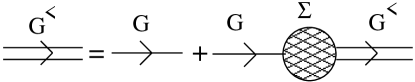
FIG. 1.: Dyson equation for the propagator in terms of the bare propagator (single lines) and the self-energy (hatched circle).

where the bare propagator is given by

$$G({\bf k},\omega)^{-1}=-i\omega+\nu_{x}k_{x}^{2}+\lambda|{\bf k}_{\perp}|^{1+\mu}\ ,$$ (57)

and the self-energy $\Sigma({\bf k},\omega)$ must be calculated perturbatively in $\gamma$. From the relation,

$$G^{<}({\bf k},\omega)^{-1}=G({\bf k},\omega)^{-1}-\Sigma({\bf k},\omega)\ ,$$ (58)

we clearly see that the perturbative corrections to $\nu_{x}$ come from terms of order $k_{x}^{2}$ in $\Sigma({\bf k},\omega)$. Setting $b=e^{l}$, with $l$ infinitesimal, equations (50) and (58) yield,

$$\frac{d\nu_{x}}{dl}=\nu_{x}\left[(z-2)-\lim_{{\bf k}\to 0}\,\frac{1}{\nu_{x}\,k_{x}^{2}\,l}\,\Sigma({\bf k},0)\right]\ .$$ (59)

The standard one-loop diagram for the self-energy is shown in Figure 2 (see, for example, [10]).

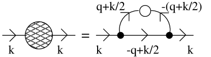
FIG. 2.: One-loop contribution to the self-energy. The internal lines also carry frequency labels (not shown).

Full circles represent $\gamma$-vertices, open circles represent contractions of the noise, $\langle\eta_{\bf k}\eta_{-\bf k}\rangle\sim D$, and arrows are bare propagators. The leading term of the self-energy in the limit $({\bf k},\omega)\to 0$ is given by

$$\Sigma({\bf k},0)=-\gamma^{2}D\int_{\Omega,q^{>}}k_{x}\left(\frac{k_{x}}{2}-q_{x}\right)\left|G\left(\frac{{\bf k}}{2}+{\bf q},\Omega\right)\right|^{2}G\left(\frac{{\bf k}}{2}-{\bf q},\Omega\right)\left|\frac{{\bf k}_{\perp}}{2}+{\bf q}_{\perp}\right|=\\ -\frac{2(6+2\mu-d)}{\mu+5-d}\,U\ \nu_{x}\,k_{x}^{2}\,l$$ (60)

$$U=\frac{S_{d-2}}{8(\mu+1)(2\pi)^{d-2}}\,\Gamma\left(\frac{d+\mu-3}{\mu+1}\right)\Gamma\left(\frac{6+2\mu-d}{\mu+1}\right)\,\gamma^{2}D\,\lambda^{\frac{3-d-\mu}{\mu+1}}\,\nu_{x}^{-\frac{6+2\mu-d}{\mu+1}}\ .$$ (61)

In the expression above $\Gamma(u)$ is the gamma function and $S_{d-2}$ is the surface area of the unit sphere in $d-2$ dimensions. The notation $(\Omega,q^{>})$ means that we integrate with the measure $d\Omega\,dq_{x}\,d{\bf q}_{\perp}/(2\pi)^{d-1}$, within the outer shell $\Lambda e^{-l}<|q_{x}|<\Lambda$. Due to the anisotropic nature of the non-linearity, there is no need to introduce a cut-off for ${\bf q}_{\perp}$. Furthermore, we have taken $\Lambda=1$ without loss of generality.

Putting together equations (59), (60) and (61), and using the scaling dimensions of the parameters $\gamma,\lambda$ and $D$, we finally obtain the RG flow equation for the effective coupling constant $U$,

$$\frac{dU}{dl}=\frac{9+\mu-2d}{\mu+1}\,U-\frac{2(6+2\mu-d)^{2}}{(\mu+1)(\mu+5-d)}\,U^{2}\ .$$ (62)

Consistent with our previous determination of the critical dimension, we see that the linear term in the flow equation changes sign for $d=d_{c}=(9+\mu)/2$. Moreover, the quadratic term is negative, implying that for any $d<d_{c}$ there is a non-zero stable fixed point $U^{\star}=O(\epsilon)$, with $\epsilon=d_{c}-d$. The RG perturbative expansion is thus well behaved and the fixed point values of $\gamma,\lambda$ and $D$ for $d<d_{c}$ are finite. The exponents (55) are therefore correct. On the other hand, for $d>d_{c}$ the only stable fixed point is $U^{\star}=0$, corresponding to an irrelevant non-linearity and thus giving the ‘free’ exponents of (53).

B The case $\mu<1$

For $\mu<1$, equation (53) gives $\zeta>1$ for the free theory, violating the assumption $\zeta<1$ under which (53) was derived. This suggests we look for a solution with $\zeta\geq 1$. In this case, $k_{x}$ will dominate over (or be the same order as) ${\bf k}_{\bot}$ in $|{\bf k}|$. The recursion relations for $\lambda$, $\nu_{x}$ and $D$ become

$$\lambda^{\prime} = b^{z-(1+\mu)}\,\lambda$$ (63)

$$\nu_{x}^{\prime} = b^{z-2}\,\nu_{x}+\cdots$$ (64)

$$D^{\prime} = b^{z-2\chi-1-(\mu-1)-(d-2)\zeta}\,D$$ (65)

instead of (49)–(51). At the fixed point of the free theory ($\gamma=0$), equation (63) gives $z=1+\mu$, so that (64) becomes $\nu_{x}^{\prime}=b^{\mu-1}\nu_{x}$, i.e. $\nu_{x}$ is driven to zero, since $\mu<1$. The theory with $\nu_{x}=0=\gamma$ is completely isotropic, so $\zeta=1$. Inserting $z=1+\mu$ and $\zeta=1$ in (65) gives $\chi=(3-d)/2$. Summarising, the exponents of the free theory for $\mu<1$ are

$$z_{0}=1+\mu\ ,\ \ \zeta_{0}=1\ ,\ \ \chi_{0}=(3-d)/2\ ,$$ (66)

which coincides with (53) in the limit $\mu\to 1$.

The relevance of $\gamma$ is again determined by equation (48). From (66), the combination $\chi+z-1$ is given, for the free theory, by $\chi_{0}+z_{0}-1=(3+2\mu-d)/2$. Hence, for $\mu<1$, $\gamma$ is relevant below the new critical dimension

$$d_{c}^{\prime}=3+2\mu\ ,\ \ \ \mu<1\ .$$ (67)

Note that $d_{c}^{\prime}$ differs from the critical dimension $d_{c}$ found for the case $\mu\geq 1$ in (54), namely $d_{c}^{\prime}<d_{c}$. On the other hand they coincide in the limit $\mu\to 1$.

For $d<d_{c}^{\prime}$, from (55) one again obtains $\zeta<1$ and therefore it is tempting to conclude that these are the correct exponents even for the $\mu<1$ case, provided that $d<d_{c}^{\prime}$. As a further consistency check, one may note that these exponents reproduce the ones of the free theory given by (66) for $d\to d_{c}^{\prime}$. Unfortunately, the situation is not as simple as this. If we perform a one-loop perturbative expansion below $d_{c}^{\prime}$, we formally get the same flow equation (62), since $\zeta<1$ in this regime. However, as we have seen, the fixed point of this equation is of order $\epsilon=d_{c}-d$, which is not small for $d\sim d_{c}^{\prime}$. In other words, because of the gap between $d_{c}^{\prime}$ and $d_{c}$, the one-loop expansion in the form stated above is not under control in the regime $\mu<1$. We were not able to find a perturbatively consistent solution in this phase. As a consequence, we can only conjecture that the exponents we have found for $\mu<1$ are correct, since they lack a substantial perturbative support.

Finally, let us note that although one can formally find a solution with $\zeta>1$, all the terms involving ${\bf k}_{\bot}$ drop out at this fixed point, and the equation becomes essentially one-dimensional, which is unphysical. We therefore reject this possibility.

C The case $d=2$

Some of the results derived above only hold for $d>2$. This is because the idea that ${\bf k}_{\bot}$ dominates $k_{x}$ in $|{\bf k}|$ is clearly inapplicable in $d=2$, since there is only $k_{x}$. Similarly, the exponent $\zeta$ can no longer be defined, so there are just two independent exponents, $z$ and $\chi$. The equation of motion and noise correlator are given by (46) and (47) respectively, but with $|{\bf k}|$ replaced by $|k_{x}|$. We recall that model H ($\mu=0$) is ill-defined for $d=2$.

The RG recursion relations for $d=2$ become,

$$\gamma^{\prime} = b^{\chi+z-1}\,\gamma$$ (68)

$$\lambda^{\prime} = b^{z-\mu-1}\,\lambda$$ (69)

$$\nu_{x}^{\prime} = b^{z-2}\,\nu_{x}+\cdots$$ (70)

$$D^{\prime} = b^{z-2\chi-\mu}\,D$$ (71)

$$D_{x}^{\prime} = b^{z-2\chi-3}\,D_{x}+\cdots,$$ (72)

Equations (68), (69) and (71) are exact, and therefore it seems that we have three equations for just two unknown exponents, $\chi$ and $z$. This apparent paradox is solved if one of the parameters is zero at the fixed point, since in this case the corresponding equation is trivially satisfied without setting the scaling dimension to zero, The shear rate $\gamma$ is certainly relevant, since $d=2$ is below the critical dimension. If we assume $D\to 0$, using equations (68) and (69) we get $\chi+z=1$ and $z=\mu+1$, giving $\chi=-\mu$. This would imply a positive scaling dimension for $D$, which is inconsistent with $D\to 0$. Thus, we must assume $\lambda\to 0$, and find from equations (68) and (71), $\chi+z=1$ and $z-2\chi=\mu$ at the fixed point, giving

$$z=(2+\mu)/3\ ,\ \ \ \chi=(1-\mu)/3$$ (73)

in $d=2$. Inserting these results into (69) gives $\lambda^{\prime}=b^{-(1+2\mu)/3}\lambda$, so $\lambda$ flows to zero in $d=2$, as assumed, for all $\mu>-1/2$.

IV stability of the domains

The calculations of the previous sections are important to assess the stability of the highly stretched domains in a coarsening system under shear. We recall that we are considering a shear velocity profile with flow in the $x$ direction and gradient in the $y$ direction. We denote by $\bf x_{\perp}$ all the directions orthogonal to both $x$ and $y$ for $d\geq 3$. The effect of the shear is to stretch the coarsening domains, such that there are two different length scales, $L_{\parallel}$, along the $x$ direction, and $L_{\perp}$ in all the orthogonal directions. The transverse size of the domains, $L_{\perp}$, is in general much smaller than longitudinal one, $L_{\parallel}$ [2, 3]. What we have to check is whether the size $\Delta$ of the height fluctuation is larger than $L_{\perp}$, inducing a breaking of the domains, or whether $\Delta<L_{\perp}$, meaning that the domains are stable under thermal fluctuations.

In the long-time limit, the main orientation of the domains will be almost completely parallel to the shear flow, and therefore height fluctuations in the surface of the domains grow in a direction orthogonal to $x$. In $d=2$, this implies that the only relevant fluctuations are in the $y$, that is $h$, direction. On the other hand, for $d=3$, there are also fluctuations growing in the $\bf x_{\perp}$ direction, which are not described by equation (1). These two cases will therefore be treated separately.

A The case $d=2$

In two dimensions the height fluctuations of the surface are given by the fluctuations of the field $h$. Thus, as a consequence of the scaling relation $h(x,t)=b^{\chi}h^{\prime}(x^{\prime},t^{\prime})$ (see Eq. (45)), the height fluctuation $\Delta$ grows as

$$\Delta\sim h\sim t^{\chi/z}F(t/L_{\parallel}^{z})\ ,$$ (74)

where the scaling function $F$ goes to a constant for small argument and $F(s)\sim s^{-\chi/z}$ for $s\to\infty$. This means that if $t^{1/z}\ll L_{\parallel}$ the surface grows like $\Delta\sim t^{\chi/z}$, whereas if $t^{1/z}\gg L_{\parallel}$, we have $\Delta\sim L_{\parallel}^{\chi}$. We can incorporate both limits in the form

$$\Delta\sim\min\left(t^{\chi/z},L_{\parallel}^{\chi}\right)\ .$$ (75)

In two dimensions we need only consider models A ($\mu=1$) and B ($\mu=2$).

1 Model A

In this case the critical dimension is $d_{c}=5$, so for $d=2$ the shear is relevant. From the former sections we have $\chi=0$ and $z=1$. Equation (75) therefore implies that, whatever value $L_{\parallel}$ takes, the height fluctuation $\Delta$ will be of order unity. In [6] it has been shown that for model A the transverse domain size is $L_{\perp}\sim O(1)$. This is an analytical result obtained in the context of the Ohta-Jasnow-Kawasaki approximation. This gives,

$$\Delta\sim L_{\perp}\quad\quad(d=2\ ,\quad\quad{\rm Model\ A})\ .$$ (76)

We conclude that model A in two dimensions is a marginal case, and we cannot exclude the possibility that thermal fluctuations may in this case break the domains, giving rise to a stationary state.

2 Model B

For model B we have $d_{c}=11/5>2$, and the exponents are $\chi=-1/3$, $z=4/3$. Also in this case, therefore, we do not need to know the coarsening exponent for $L_{\parallel}$, since from relation (75) it is clear that a negative value of $\chi$ implies a saturation of $\Delta$ to a constant value:

$$\Delta\sim O(1)\quad\quad(d=2\ ,\quad\quad{\rm Model\ B})\ .$$ (77)

This result opens up two different scenarios, according to the the growth law for $L_{\perp}$. If $L_{\perp}\sim t^{1/3}$, as argued in [4] by means of numerical experiments and RG arguments, then $\Delta\ll L_{\perp}$ and the domains must be stable against thermal fluctuations. If, however, $L_{\perp}\sim O(1)$, as suggested by some recent numerical simulations [8], then, as in model A, we cannot exclude the possibility that a breaking of the domains by thermal fluctuations occurs. Our result shows that a $L_{\perp}\sim t^{1/3}$ growth law and a thermally induced stretching and breaking mechanism are not compatible. Conversely, if a thermally-induced breaking of the domains is clearly observed in numerical experiments, this strongly suggests that the relation $L_{\perp}\sim O(1)$ holds.

B The case $d=3$

In three dimensions the situation is more complicated. First, as in $d=2$, there are height fluctuations in the $y$ direction, $\Delta_{y}\sim h$, described by equation (1). Secondly, there are fluctuations in the $x_{\perp}$ direction, $\Delta_{\perp}$, which can also become larger than $L_{\perp}$, and that are not described by equation (1). Thus, before assessing the stability of the domains for $d=3$ we must formulate an equation for the description of these latter fluctuations. Fortunately, this will turn out to be a linear equation, such that no perturbative RG analysis is necessary.

In order to describe surface fluctuations which grow in the $x_{\perp}$ direction we have to introduce a new height field $h_{\perp}$ which satisfies the equation,

$$\partial_{t}h_{\perp}+\gamma y\partial_{x}h_{\perp}={\cal L}h_{\perp}+\eta\ ,$$ (78)

to be compared with (1). The operator $\cal L$ is still given at low momenta by ${\cal L}\sim\lambda|{\bf k}|^{1+\mu}$. Equation (78) is linear, and therefore we can work out the exponents exactly by means of simple scaling. By setting,

$$x=bx^{\prime},\ \ y=b^{\zeta}y^{\prime},\ \ h_{\perp}=b^{\chi}h_{\perp}^{\prime},\ \ t=b^{z}t^{\prime}\ ,$$ (79)

and imposing scale invariance of equation (78), we obtain (with the usual hypothesis $\zeta<1$),

$$\gamma^{\prime} = b^{z-1+\zeta}\,\gamma$$ (80)

$$\lambda^{\prime} = b^{z-\zeta(\mu+1)}\lambda$$ (81)

$$D^{\prime} = b^{z-2\chi-\zeta\mu-1}D\ ,$$ (82)

and setting to zero the scaling dimensions of all three parameters gives

$$z=\frac{\mu+1}{\mu+2},\ \ \zeta=\frac{1}{\mu+2},\ \ \chi=-\frac{\mu+1}{2(\mu+2)}\ .$$ (83)

Note that $\zeta$ is smaller than one, consistent with our assumption. We see that $\chi$ is negative for all the three interesting values of $\mu$ ($\mu=0,1,2$), meaning that height fluctuations along the $x_{\perp}$ direction are always finite, $\Delta_{\perp}\sim O(1)$.

We have to assess now the physical importance of $\Delta_{y}$ in the context of domain coarsening. From the usual scaling relations we get,

$$\Delta_{y}\sim h\sim t^{\chi/z}F(t/L_{\parallel}^{z},\ t/L_{\perp}^{z/\zeta})\ .$$ (84)

In general, evaluating the magnitude of $\Delta_{y}$ from this relation is quite subtle, as we need to compare the interfacial coarsening and equilibrium regimes in both the parallel and perpendicular directions. However, as we discuss below, in all cases of physical interest we have $\chi\leq 0$, implying that the interfacial fluctuations saturate.

1 Model A

In the case $\mu=1$ and $d=3$, Eq. (55), with $\mu=1$, gives $\chi=-1/5$, and therefore $\Delta_{y}\sim O(1)$. For model A it was been found in [6] that $L_{\perp}\sim t^{1/2}$, giving

$$\Delta_{y}\ll L_{\perp}\quad\quad(d=3\ ,\quad\quad{\rm Model\ A})\ .$$ (85)

In model A, domains are therefore stable against thermal fluctuations.

2 Model B

In this case also the exponent $\chi$ is negative: Eq. (55) with $\mu=2$ gives $\chi=-2/7$, and $z=9/7$, yielding

$$\Delta_{y}\sim O(1)\quad\quad(d=3\ ,\quad\quad{\rm Model\ B})\ .$$ (86)

Even though no analytical results or numerical simulations studies are available at the present time for model B in $d=3$, we certainly expect $L_{\perp}$ to grow with time in this case, and therefore the domains to be stable.

3 Model H

For $\mu<1$, as we have seen, we have a different critical dimension, given by Eq. (67), which is exactly three for $\mu=0$. This implies, using either (66) or (55), that $\chi=0$ and $z=1$. Once again, this is the marginal case, with

$$\Delta_{y}\sim O(1)\quad\quad(d=3,\quad\quad{\rm Model\ H})\ .$$ (87)

V Summary

Interfacial fluctuations have been investigated in systems subjected to an external shear flow. Interfacial dynamics appropriate to systems with non-conserved scalar order parameter (“model A”), conserved scalar order parameter (“model B”), and conserved scalar order parameter coupled to hydrodynamic flow (“model H”) have been studied. In each case the interfacial dynamics is described by a similar equation, of the form (1), where $h$ is the local height of the interface and in which the eigenvalue spectrum of the linear operator $\cal{L}$ has the form (2). The models differ principally in the numerical value of the exponent $\mu$, which is given by 1,2 and 0 for models $A$, $B$ and $H$ respectively.

The interface equations have the form of anisotropic noisy Burgers equations. In each case, exact renormalization group (RG) arguments determine the exponents $z$, $\zeta$, and $\chi$ that characterise the coarsening, anisotropy, and roughening of the interface respectively. In all cases, $\chi\leq 0$, implying that the thermally induced interfacial width approaches a finite limit at infinite time. A consequence of this result is that the domain structure of a coarsening system under shear is stable against (sufficiently weak) thermal fluctuations.

The general framework revealed by the exact RG relations was supported by explicit one-loop calculations for $\mu\geq 1$. For $\mu<1$, however, no one-loop equations consistent with the expected critical dimension, $d_{c}^{\prime}=3+2\mu$, could be derived. Whether this is just a technical difficulty, or signals some important physical difference between the regimes $\mu\geq 1$ and $\mu<1$, merits further investigation.

ACKNOWLEDGEMENTS

AC thanks Antti Kupiainen for a useful discussion. This work was supported by EPSRC grant GR/L97698 (AJB and AC), and by Fundação para a Ciência e a Tecnologia grant BD/21760/99 (RDMT).

REFERENCES

- [1] A.J. Bray, Adv. Phys. 43, 357 (1994), and references therein.
- [2] T. Hashimoto, K. Matsuzaka, E. Moses, and A. Onuki, Phys. Rev. Lett. 74, 126 (1995); J. Läuger, C. Laubner, and W. Gronski, Phys. Rev. Lett. 75, 3576 (1995).
- [3] T. Ohta, H. Nozaki, and M. Doi, J. Chem. Phys. 93, 2664 (1991); Y. N. Wu, H. Skrdla, T. Lookman, and S. Y. Chen, Physica A 239 (1-3), 428 (1997); A. J. Wagner and J. M. Yeomans, Phys. Rev. E 59, 4366 (1999); F. Corberi, G. Gonnella, and A. Lamura, Phys. Rev. Lett. 81, 3852 (1998); Phys. Rev. E 62, 6621 (2000); ibid. 8064 (2000); N. P. Rapapa and A. J. Bray, Phys. Rev. Lett. 83, 3856 (1999).
- [4] F. Corberi, G. Gonnella, and A. Lamura, Phys. Rev. Lett. 83, 4057 (1999).
- [5] P. Padilla and S. Toxvaerd, J. Chem. Phys. 106, 2342 (1997).
- [6] A. J. Bray and A. Cavagna, J. Phys. A 33, L305 (2000); A. Cavagna, A. J. Bray, and R. D. M. Travasso, Phys. Rev. E 62, 4702 (2000).
- [7] Z. Y. Shou and A. Chakrabarti, Phys. Rev. E, 61, R2200 (2000).
- [8] L. Berthier, Phys. Rev. E 63, 051503 (2001).
- [9] J. M. Burgers, The nonlinear Diffusion Equation (Reidel, Boston, 1974).
- [10] D. Forster, D. R. Nelson, and M. J. Stephen, Phys. Rev. A 16, 732 (1977).
- [11] P.C. Hohenberg, and B.I. Halperin, Rev. Mod. Phys. 49, 435 (1977).
- [12] S. F. Edwards and D. R. Wilkinson, Proc. R. Soc. London, Ser. A 381, 17 (1982).
- [13] J. S. Langer and L. A. Turski, Acta. Metall. 25, 1113 (1977); D. Jasnow and R. K. P. Zia, Phys. Rev. A 36, 2243 (1987); A. Shinozaki and Y. Oono, Phys. Rev. E 47, 804 (1993).
- [14] A. Shinozaki, Phys. Rev. E 48, 1984 (1993).
- [15] A. J. Bray, Phys. Rev. E 58, 1508 (1998).
- [16] E. D. Siggia, Phys. Rev. A 20, 595 (1979).
- [17] H. Furukawa, Phys. Rev. A 31, 1103 (1985).
- [18] A. J. Bray, A. Cavagna, and R. D. M. Travasso, Phys. Rev. E, in press.
- [19] T. Hwa and M. Kardar, Phys. Rev. A 45, 7002 (1992). See also V. Becker and H. K. Janssen, Phys. Rev. E 50, 1114 (1994).