Abstract

We present a simple two-dimensional dynamical system where two nonlinear terms, exerting respectively positive feedback and reversal, compete to create a singularity in finite time decorated by accelerating oscillations. The power law singularity results from the increasing growth rate. The oscillations result from the restoring mechanism. As a function of the order of the nonlinearity of the growth rate and of the restoring term, a rich variety of behavior is documented analytically and numerically. The dynamical behavior is traced back fundamentally to the self-similar spiral structure of trajectories in phase space unfolding around an unstable spiral point at the origin. The interplay between the restoring mechanism and the nonlinear growth rate leads to approximately log-periodic oscillations with remarkable scaling properties. Three domains of applications are discussed: (1) the stock market with a competition between nonlinear trend-followers and nonlinear value investors; (2) the world human population with a competition between a population-dependent growth rate and a nonlinear dependence on a finite carrying capacity; (3) the failure of a material subjected to a time-varying stress with a competition between positive geometrical feedback on the damage variable and nonlinear healing.

1 Introduction

The mathematics of singularities is applied routinely in the physics of phase transitions to describe for instance the transformations from ice to water or from a magnet to a demagnetized state when raising the temperature, as well as in many other condensed matter systems. Such singularities characterize so-called critical phenomena. In these problems, physical observables such as susceptibilities, specific heat, etc., exhibit a singularity as the control parameter (temperature, strength of the interaction) approaches a critical value.

Other classes of singularities occur in dynamical systems and are spontaneously reached in finite time. Spontaneous singularities in ordinary (ODE) and partial differential equations (PDE) are quite common and have been found in many well-established models of natural systems, either at special points in space such as in the Euler equations of inviscid fluids [45, 4], in the surface curvature on the free surface of a conducting fluid in an electric field [59], in vortex collapse of systems of point vortices, in the equations of General Relativity coupled to a mass field leading to the formation of black holes [11], in models of micro-organisms aggregating to form fruiting bodies [46], or in the more prosaic rotating coin (Euler’s disk) [42]. Some more complex examples are models of rupture and material failure [25, 29], earthquakes [32] and stock market crashes [31, 28].

The normal form of a finite-time singularity is the equation

$${dp\over dt}=p^{m}~{},~{}~{}~{}~{}~{}~{}~{}{\rm with}~{}m>1~{},$$ (1)

whose solution is

$$p(t)=p(0)~{}\left({t_{c}-t\over t_{c}}\right)^{-1/(m-1)}~{},$$ (2)

where the critical time $t_{c}=(m-1)/[p(0)]^{m-1}$ is determined by the initial condition $p(0)$. The singularity results from the fact that the instantaneous growth rate $d\ln p/dt=p^{m-1}$ is increasing with $p$ and thus with time. This can be visualized by studying the doubling time, defined at the time interval $\Delta t$ necessary for $p(t)$ to double, i.e., $p(t+\Delta t)=2p(t)$. When the growth rate of $p$ increases as a power law of $p$, the doubling time decreases fast and the sequence of doubling time intervals shrinks to zero sufficiently fast so that its sum is a convergent geometrical series. The variable thus undergoes an infinite number of doubling operations in a finite time, which the essence of a finite-time singularity.

The power law solution (2) possesses the symmetry of “scale invariance”, namely a reduction $t_{c}-t\to(t_{c}-t)/\lambda$ of the distance $t_{c}-t$ from the singularity at $t_{c}$ by an arbitrary factor $\lambda$ changes $p(t)$ to $\lambda^{1/(m-1)}~{}p(t)$, i.e., keeps the same form of the solution up to a global rescaling.

This continuous scale invariance can be partially broken into a weaker symmetry, called discrete scale invariance, according to which the self-similarity holds only for integer powers of a specific factor $\lambda$ [49]. The hallmark of this discrete scale invariance is that the power law (2) transforms into an oscillatory singularity, with log-periodic oscillations decorating the overall power law acceleration. Such log-periodic power laws have been documented for many systems such as with a built-in geometrical hierarchy, in programming and number theory, for Newcomb-Benford law of first digits and in the arithmetic system, in diffusion in anisotropic quenched random lattices, as the result of a cascade of ultra-violet instabilities in growth processes and rupture, in deterministic dynamical systems (cascades of sub-harmonic bifurcations in the transition to chaos, two-coupled anharmonic oscillators, near-separatrix Hamiltonian chaotic dynamics, kicked charged particle moving in a double-well potential giving a physical realization of Mandelbrot and Julia sets, chaotic scattering), in extension of percolation theory (so-called “animals”), in response functions of spin systems with quenched disorder, in freely decaying 2D-turbulence, in the gravitational collapse and black hole formation, in spinodal decomposition of binary mixtures in uniform shear flow, etc. (see [49, 51] and references therein).

The novel interesting feature is the presence of a discrete hierarchy of length and/or time scales in an otherwise scale-invariant system. The presence of these scales may provide insight into the underlying mechanisms. While there is a good general framework for the description of discrete scale invariant systems using renormalization group theory [49], a general understanding of the possible physical mechanisms at its origin is still lacking. In particular, dynamically generated discrete scale invariance is the most important problem, as it might provide understanding in the origins of the ubiquitous existence of hierarchies and cascades in natural and social systems.

Here, we introduce and study a simple two-dimensional nonlinear dynamical system with the minimal ingredients ensuring that it exhibits both a finite-time singularity (and its associated scale invariance) and oscillatory behavior. The scale invariance is thus partially broken by the existence of dynamically generated length scales associated with the oscillations. We start from (1) and enrich it by the minimal ingredient to obtain what we believe is the simplest “normal form” of an oscillatory finite-time singularity. While the singularity emerges from the nonlinear growth law with positive feedback, the hierarchy of length scales results from a nonlinear negative feedback. The competition between the positive and negative nonlinear feedbacks create an approximate self-similar oscillatory structures, which can be understood from a spiral dynamics in phase space around a central unstable fixed point. Physically, the self-similar oscillations result from the dependence of the local frequency of the nonlinear oscillator on the amplitude. This will be shown in phase space to result from the special role played by the origin which is the unstable fixed point around which the spiral structures of trajectories are organized.

This spiral structure of the dynamics around the central unstable fixed point bears a superficial resemblance to the the Shilnikov’s mechanism for chaos [22]. However, both their dynamics and their behaviors are unrelated. Shilnikov’s systems are characterized by trajectories in phase space spiraling towards the hyperbolic point along the stable manifold and then blowing-up exponentially along the unstable manifold of the hyperbolic point, until they are reinjected again along the stable manifold. In our system, trajectories in phase space spiral out slowly at first and then accelerate until a singular point in finite-time is reached due to a faster-than-exponential acceleration. Our system has thus a finite lifetime while Shilnikov’s systems are globally statistically stationary.

Our work is somewhat more related to that of several authors who emphasized the possible role of spiral structures in singular flows as a mechanism to promote the transfer of energy from large scales to small scales [4, 58, 24]. Kiehn [34] has emphasized that vortex sheet evolution, governed by an integral form of the Biot-Savart law (known as the Rott-Birchoff equation) leads to the production of discontinuities in finite time. Asymptotic spiral type solutions in the vicinity of the singularity have been investigated both analytically and numerically (see [34] and references therein). Szydlowski et al. [54] have analyzed a nonlinear second-order ordinary differential equation, called the Kaldor-Kalecki business model in which capital stock changes are caused by past investment decisions. Their study emphasizes the negative feedback connected with the lag-delay effect and thus lacks the positive feedback trend effect discussed here. Canessa [6, 7] has also a nonlinear second-order differential equation for the price but again the emphasis is on the nonlinear feedback rather than on the possibility of explosive phases coupled with the oscillatory behavior.

Let us also mention another mechanism for log-periodicity: scale invariant equations which present an instability at finite wavevector decreasing with the field amplitude may generate naturally a discretely scale-invariant spectrum of internal scales [50].

We first motivate the normal form studied here for an oscillatory finite-time singularity by three physical examples, namely the time evolution of a stock market price described in section 2, the dynamics of human population described in section 3 and the coupled evolution of a damage variable and the average stress leading to material rupture given in section 4. We then present in section 5 an analysis of the effect of each of the two components (the nonlinear amplification and the nonlinear reversal term) of the dynamics taken separately. Section 6 describes in a rather heuristic way the fundamental characteristics of the overall dynamics obtained when combining both terms. Section 7 provides a detailed dynamical system approach giving a complete characterization of the dynamics in phase space and precise predictions on the exponents of the scaling laws which are tested by numerical simulations. Section 8 concludes.

2 Stock market price dynamics

The importance of the interplay of two classes of investors, so-called fundamental value investors and technical analysists (or trend followers), has been stressed by several recent works [40, 16] to be essential in order to retrieve the important stylized facts of stock market price statistics. We build on this insight and construct a simple model of price dynamics, whose innovation is to put emphasis on the fundamental nonlinear behavior of both classes of agents.

2.1 Nonlinear value and trend-following strategies

The variation of price of an asset on the stock market is controlled by supply and demand, in other words by the net order size $\Omega$ through a market impact function [15]. Assuming that the ratio ${\tilde{p}}/p$ of the price ${\tilde{p}}$ at which the orders are executed over the previous quoted price $p$ is solely a function of $\Omega$ and using the condition that it is impossible to make profits by repeatedly trading through a close circuit (i.e. by buying and selling with final net position equal to zero), Farmer [15] has shown that the logarithm of the price is given by the following equation written in discrete form

$$\ln p(t+1)-\ln p(t)={\Omega(t)\over L}~{}.$$ (3)

The so-called “market depth” $L$ is the typical number of outstanding stocks traded per unit time and thus normalizes the impact of a given order size $\Omega(t)$ on the log-price variations. The net order size $\Omega$ summed over all traders is changing as a function of time so as to reflect the information flow in the market and the evolution of the traders’ opinions and moods. A zero net order size $\Omega=0$ corresponds to exact balance between supply and demand. Various derivations have established a connection between the price variation or the variation of the logarithm of the price to factors that control the net order size itself [15, 5, 44]. Two basic ingredients of $\Omega(t)$ are thought to be important in determining the price dynamics: reversal to the fundamental value ($\Omega_{\rm fund}(t)$) and trend following ($\Omega_{\rm trend}(t)$). Other factors, such as risk aversion, may also play an important role.

We propose to describe the reversal to estimated fundamental value by the contribution

$$\Omega_{\rm fund}(t)=-c~{}[\ln p(t)-\ln p_{f}]~{}|\ln p(t)-\ln p_{f}|^{n-1}~{},$$ (4)

to the order size, where $p_{f}$ is the estimated fundamental value and $n>0$ is an exponent quantifying the nonlinear nature of reversion to $p_{f}$. The strength of the reversion is measured by the coefficient $c>0$, which reflects that the net order is negative (resp. positive) if the price is above (resp. below) $p_{f}$. The nonlinear power law $[\ln p(t)-\ln p_{f}]~{}|\ln p(t)-\ln p_{f}|^{n-1}$ of order $n$ is chosen as the simplest function capturing the following effect. In principle, the fundamental value $p_{f}$ is determined by the discounted expected future dividends and is thus dependent upon the forecast of their growth rate and of the risk-less interest rate, both variables being very difficult to predict. The fundamental value is thus extremely difficult to quantify with high precision and is often estimated within relatively large bounds [41, 10, 38, 8]: all of the methods of determining intrinsic value rely on assumptions that can turn out to be far off the mark. For instance, several academic studies have disputed the premise that a portfolio of sound, cheaply bought stocks will, over time, outperform a portfolio selected by any other method (see for instance [37]). As a consequence, a trader trying to track fundamental value has no incentive to react when she feels that the deviation is small since this deviation is more or less within the noise. Only when the departure of price from fundamental value becomes relatively large will the trader act. The relationship (4) with an exponent $n>1$ precisely accounts for this effect: when $n$ is significantly larger than $1$, $|x|^{n}$ remains small for $|x|<1$ and shoots up rapidly only when it becomes larger than $1$, mimicking a smoothed threshold behavior. The nonlinear dependence of $\Omega_{\rm fund}(t)$ on $\ln[p(t)/p_{f}]=\ln p(t)-\ln p_{f}$ shown in (4) is the first novel element of our model. Usually, modelers reduce this term to the linear case $n=1$ while, as we shall show, generalizing to larger values $n>1$ will be a crucial feature of the price dynamics. In economic language, the exponent $n=d\ln\Omega_{\rm fund}/d\ln\left(\ln[p(t)/p_{f}]\right)$ is called the “elasticity” or “sensitivity” of the order size $\Omega_{\rm fund}$ with respect to the (normalized) l0g-price $\ln[p(t)/p_{f}]$.

A related “sensitivity”, that of the money demand to interest rate, has has been recently documented to be larger than $1$, similarly to our proposal of taking $n>1$ in (4). Using a survey of roughly 2,700 households, Mulligan and Sala-i-Martin [43] estimated the interest elasticity of money demand (the sensitivity or log-derivative of money demand to interest rate) to be very small at low interest rates. This is due to the fact that few people decide to invest in interest-producing assets when rates are low, due to “shopping” costs. In contrast, for large interest rates or for those who own a significant bank account, the interest elasticity of money demand is significant. This is a clear-cut example of a threshold-like behavior characterized by a strong nonlinear response. This can be captured by $e\equiv d\ln M/d\ln r=(r/r_{\rm infl})^{n}$ with $n>1$ such that the elasticity $e$ of money demand $M$ is negligible when the interest $r$ is not significantly larger than the inflation rate $r_{\rm infl}$ and becomes large otherwise.

Trend following (in various elaborated forms) was (and probably is still) one of the major strategy used by so-called technical analysts (see [1] for a review and references therein). More generally, it results naturally when investment strategies are positively related to past price moves. Trend following can be captured by the following expression of the order size

$$\Omega_{\rm trend}(t)=a_{1}[\ln p(t)-\ln p(t-1)]+a_{2}[\ln p(t)-\ln p(t-1)]|\ln p(t)-\ln p(t-1)|^{m-1}~{}.$$ (5)

This expression corresponds to driving the price up if the preceding move was up ($a_{1}>0$ and $a_{2}>0$). The linear case $(a_{1}>0,a_{2}=0)$ is usually chosen by modelers. Here, we generalize this model by adding the contribution proportional to $a_{2}>0$ from considerations similar to those leading to the nonlinear expression (4) for the reversal term with an exponent $n>1$. We argue that the dependence of the order size at time $t$ resulting from trend-following strategies is a nonlinear function with exponent $m>1$ of the price change at previous time steps. Indeed, a small price change from time $t-1$ to time $t$ may not be perceived as a significant and strong market signal. Since many of the investment strategies are nonlinear, it is natural to consider an average trend-following order size which increases in an accelerated manner as the price change increases in amplitude. Usually, trend-followers increase the size of their order faster than just proportionally to the last trend. This is reminiscent of the argument [1] that traders’s psychology is sensitive to a change of trend (acceleration or deceleration) and not simply to the trend (velocity). The fact that trend-following strategies have an impact on price proportional to the price change over the previous period raised to the power $m>1$ means that trend-following strategies are not linear when averaged over all of them: they tend to under-react for small price changes and over-react for large ones. The second term with coefficient $a_{2}$ captures this phenomenology.

2.2 Nonlinear dynamical equation for stock market prices

Introducing the notation

$$x(t)=\ln[p(t)/p_{f}]~{},$$ (6)

and the time scale $\delta t$ corresponding to one time step, and putting all the contributions (4) and (5) into (3), with $\Omega(t)=\Omega_{\rm fund}(t)+\Omega_{\rm trend}(t)$, we get

$$x(t+\delta t)-x(t)={1\over L}\left(a_{1}~{}[x(t)-x(t-\delta t)]+a_{2}[x(t)-x(t-\delta t)]|x(t)-x(t-\delta t)|^{m-1}-c~{}x(t)|x(t)|^{n-1}\right)~{}.$$ (7)

Expanding (7) as a Taylor series in powers of $\delta t$, we get

$$(\delta t)^{2}{d^{2}x\over dt^{2}}=-\left[1-{a_{1}\over L}\right]~{}\delta t~{}{dx\over dt}+{a_{2}(\delta t)^{m}\over L}{dx\over dt}|{dx\over dt}|^{m-1}-{c\over L}x(t)|x(t)|^{n-1}~{}+~{}{\cal O}[(\delta t)^{3}]~{},$$ (8)

where ${\cal O}[(\delta t)^{3}]$ represents a term of the order of $(\delta t)^{3}$. Note the existence of the second order derivative, which results from the fact that the price variation from present to tomorrow is based on analysis of price change between yesterday and present. Hence the existence of the three time lags leading to inertia. A special case of expression (7) with a linear trend-following term $(a_{2}=0)$ and a linear reversal term $(n=1)$ has been studied in [5, 15], with the addition of a risk-aversion term and a noise term to account for all the other effects not accounted for by the two terms (4) and (5). We shall neglect risk-aversion as well as any other term and focus only on the reversal and trend-following terms previously discussed to explore the resulting price behaviors. Grassia has also studied a similar linear second-order differential equation derived from market delay, positive feedback and including a mechanism for quenching runaway markets [19]. Thurner [55] considers a three-dimensional system of three ordinary differential equations coupling price, “friction” and a state variable controlling friction, which can be mapped onto a third-order ordinary differential equation. The nonlinearity is on the friction term and not on the trend term which is again assumed linear.

Expression (7) is inspired by the continuous mean-field limit of the model of Pandey and Stauffer [44], defined by starting from the percolation model of market price dynamics [14, 12, 53] and developed to account for the dynamics of the Nikkei and Russian market recessions [26, 27]. The generalization assumes that trend-following and reversal to fundamental values are two forces that influence the probability that a trader buys or sells the market. In addition, Pandey and Stauffer [44] consider as we do here that the dependence of the probability to enter the market is a nonlinear function with exponent $n>1$ of the deviation between market price and fundamental price. However, they do not consider the possibility that $m>1$ and stick to the linear trend-following case. We shall see that the analytical control offered by our continuous formulation allows us to get a clear understanding of the different dynamical phases.

Among the four terms of equation (8), the first term of the right-hand-side of (8) is the least interesting. For $a_{1}<L$, it corresponds to a damping term which becomes negligible compared to the second term in the terminal phase of the growth close to the singularity when $|dx/dt|$ becomes very large. For $a_{1}>L$, it corresponds to a negative viscosity but the instability it provides is again subdominant for $m>1$. The main ingredients here are the interplay between the inertia provided by the second derivative in the left-hand-side, the destabilizing nonlinear trend-following term with coefficient $a_{2}>0$ and the nonlinear reversal term. In order to simplify the notation and to simplify the analysis of the different regimes, we shall neglect the first term of the right-hand-side of (8), which amounts to take the special value $a_{1}=L$. In a field theoretical sense, our theory is tuned right at the “critical point” with a vanishing “mass” term.

Equation (8) can be viewed in two ways. It can be seen as a convenient short-hand notation for the intrinsically discrete equation (7), keeping the time step $\delta t$ small but finite. In this interpretation, we pose

$$\alpha = a_{2}(\delta t)^{m-2}/L~{},$$ (9)

$$\gamma = c/L(\delta t)^{2}~{},$$ (10)

which depend explicitely on $\delta t$, to get

$${d^{2}x\over dt^{2}}=\alpha{dx\over dt}|{dx\over dt}|^{m-1}-\gamma x(t)|x(t)|^{n-1}~{}.$$ (11)

A second interpretation is to genuinely take the continuous limit $\delta t\to 0$ with the constraints $a_{2}/L\sim(\delta t)^{2-m}$ and $c/L\sim(\delta t)^{2}$. This allow us to define the now $\delta t$-independent coefficients $\alpha$ and $\gamma$ according to (9) and (11) and obtain the truly continuous equation (11). This equation can also be written as

$${dy_{1}\over dt} = y_{2}~{},$$ (12)

$${dy_{2}\over dt} = \alpha y_{2}|y_{2}|^{m-1}-\gamma y_{1}|y_{1}|^{n-1}~{}.$$ (13)

This is the system we are going to study for $m>1$ and $n>1$. For further discussions, we call the term proportional to $\alpha$ (resp. $\gamma$) the trend or positive feedback term (resp. the reversal term). The richness of behaviors documented below results from the competition between these two terms.

In defining the generalized dynamics (12,13) for the market price, we aim at a fundamental dynamical understanding of the observed interplay between accelerating growth and accelerating (log-periodic) oscillations, that have been documented in speculative bubbles preceding large crashes [31, 27, 28].

We shall show below that the origin $(y_{1}=0,y_{2}=0)$ plays a special role as the unstable fixed point around which spiral structures of trajectories are organized in phase space $(y_{1},y_{2})$. It is particularly interesting that this point plays a special role since $y_{1}=0$ means that the observed price is equal to the fundamental price. If, in addition, $y_{2}=0$, there is no trend, i.e., the market “does not know” which direction to take. The fact that this is the point of instability around which the price trajectories organize themselves provides a fundamental understanding of the cause of the complexity of market price time series based on the instability of the fundamental price “equilibrium”.

3 Population dynamics

As a standard model of population growth, Malthus’ model assumes that the size of a population increases by a fixed growth rate $\sigma$ independently of the size of the population and thus gives an exponential growth:

$${dp\over dt}=\sigma p(t)~{}.$$ (14)

The logistic equation attempts to correct for the resulting unbounded exponential growth by assuming a finite carrying capacity $K(t)$ such that the population instead evolves according to

$${dp\over dt}=\sigma_{0}p(t)\left[K(t)-p(t)\right]~{},$$ (15)

where $\sigma_{0}$ controls the amplitude of the nonlinear saturation term. Applying this model to the human population on earth, Cohen and others (see [13] and references therein) have put forward idealized models taking into account interaction between the human population $p(t)$ and the corresponding carrying capacity $K(t)$ by assuming that $K(t)$ increases with $p(t)$ due to technological progress such as the use of tools and fire, the development of agriculture, the use of fossil fuels, fertilizers etc. as well an expansion into new habitats and the removal of limiting factors by the development of vaccines, pesticides, antibiotics, etc. If $K(t)$ grows faster than $p(t)$, then $p(t)$ explodes to infinity after a finite time creating a singularity [30]. In this case, the limiting factor $-p(t)$ can be dropped out and, assuming a simple power law relationship $K(t)\propto[p(t)]^{\delta}$ with $\delta>1$, (15) can be written as (14) with an accelerating growth rate $\sigma$ replacing $\sigma_{0}$:

$$\sigma=\sigma_{0}[p(t)]^{\delta}~{}.$$ (16)

The generic consequence of a power law acceleration in the growth rate is the appearance of singularities in finite time:

$$p(t)=p(0)\left({t_{c}-t\over t_{c}}\right)^{-{1\over\delta}},~{}~{}~{}~{}\mbox{for $t$ close to $t_{c}$}~{},$$ (17)

where $t_{c}$ is determined by the constant of integration, i.e., the initial condition $p(0)$ as $t_{c}=[p(0)]^{-\delta}/\delta\sigma_{0}$. Equation (16) is said to have a “spontaneous” or “movable” singularity at the critical time $t_{c}$ [3],

Note that, using (17), (16) can be written

$${d\sigma\over dt}\propto\sigma^{2}~{},$$ (18)

showing that the finite-time singularity of the population $p(t)$ is the result of the finite-time singularity of its growth rate, resulting from the quadratic growth equation (18).

We now generalize (18) as

$${d\sigma\over dt}=\alpha\sigma|\sigma|^{m-1}-\gamma\ln(p/K_{\infty})|\ln(p/K_{\infty})|^{n-1}~{}$$ (19)

for the following reasons. Apart from the absolute value, the first term in the r.h.s. of (19) is the same as (18) with $m=2$. In addition, we allow the instantaneous growth rate $\sigma$ to be negative and thus its growth has to be signed. The novel second term in the r.h.s. of (19) takes into account a saturation or restoring effect such that by itself this term attracts the population $p(t)$ to an asymptotic constant carrying capidity $K_{\infty}$. Using the logarithm of the ratio $p/K_{\infty}$ is the natural choice for the dynamics of a growth rate since $\ln(p/K_{\infty})$ is nothing but the effective cumulative growth rate. For $n=1$, $-\gamma\ln(p/K_{\infty})|\ln(p/K_{\infty})|^{n-1}=-\gamma\ln(p/K_{\infty})$ corresponds to a linear (in $\ln(p/K_{\infty})$) restoring term. A choice $n>1$ captures the following effect: the restoring term is very weak when $p$ departs weakly from $K$ and then becomes rather suddenly stronger when this deviation increases. This nonlinear feedback effect is intended to capture the many nonlinear (often quasi-threshold) feedback mechanisms acting on population dynamics. In the limit $n\to+\infty$, the reversal term acts as a threshold. Note that the absolute values can be removed when the exponents $m$ and $n$ are odd.

Expression (19) generalizes (15) by putting together a faster-than-exponential growth and an attraction to finite value. In contrast, (15) puts together an exponential growth and an attraction to a finite value.

Let us introduce the change of variable

$$y_{1} = \ln(p/K_{\infty})~{},$$ (20)

$$y_{2} = \sigma~{}.$$ (21)

The equations (14,19) then retrieve (12) and (13). For further discussions, we shall refer to the term proportional to $\alpha$ (resp. $\beta$) as the positive feedback or acceleration term (resp. the reversal term).

In defining the generalized dynamics (12) and (13) with (20) for the population, we aim at a fundamental dynamical understanding of the observed interplay between accelerating growth and accelerating (log-periodic) oscillations, that have been documented in [33, 56, 23, 30].

4 Rupture of materials with competing damage and healing

Consider the problem of so-called creep or damage rupture [35] in which a rod is subjected to uniaxial tension by a constant applied axial force $P$. The intact cross section $A(t)$ of the rod is assumed to be a function of time. The physical picture is to envision myriads of microcracks damaging progressively the rod and decreasing its effective intact cross section that can sustain stress. The problem is simplified by assuming that $A(t)$ is independent of the axial coordinate, which eliminates necking as a possible mode of failure. The considered viscous deformation is assumed to be isochoric, i.e., the rod volume remains constant during the process. This provides a geometric relation between the rod cross-sectional area and length $A_{0}L_{0}=A(t)L(t)=$ constant, which holds for all times.

The rate of creep strain $\epsilon_{c}$ can be defined as a function of geometry as

$${d\epsilon_{c}\over dt}={1\over L}{dL\over dt}=-{1\over A}{dA\over dt}~{},$$ (22)

showing that

$$\epsilon_{c}(t)=\ln{L(t)\over L_{0}}=-\ln{A(t)\over A_{0}}~{},$$ (23)

where $L_{0}=L(t_{0})$ and $A_{0}=A(t_{0})$ correspond to the underformed state $\epsilon_{c}(t_{0})=0$ at time $t_{0}$.

The rate of change of the creep strain $\epsilon_{c}(t)$ is assumed to follow the rheological Norton’s law, i.e.,

$${d\epsilon_{c}\over dt}=C\sigma^{\mu}~{},~{}~{}~{}~{}{\rm with}~{}\mu>0~{},$$ (24)

where the stress

$$\sigma=P/A$$ (25)

is the ratio of the applied force over the cross section of the rod. Eliminating $d\epsilon_{c}/dt$ between (22) and (24) and using (25) leads to $A^{\mu-1}dA/dt=-CP^{\mu}$, i.e., $A(t)=A(0)\left({t_{c}-t\over t_{c}}\right)^{1/\mu}$, where the critical failure time is given by $t_{c}=[A(0)/P]^{\mu}/(\mu C)$. The rod cross section thus vanishes in a finite time $t_{c}$ and as a consequence the stress diverges as the time $t$ goes to the critical time $t_{c}$ as

$$\sigma=P/A={P\over A(0)}\left({t_{c}-t\over t_{c}}\right)^{-{1\over\mu}}~{}.$$ (26)

Physically, the constant force is applied to a thinner cross section, thus enhancing the stress, which in turn accelerate the creep strain rate, which translates into an acceleration of the decrease of the rod cross section and so on. In other words, the finite-time singularity results from the positive feedback of the increasing stress on the thinner cross section and vice-versa. This finite-time singularity for the stress can be reformulated as a self-contained equation expressed only in terms of the stress:

$${d\sigma\over dt}=C\sigma^{\mu+1}~{}.$$ (27)

Let us now generalize this model by allowing not only creep deformations leading to damage but also recovery or healing as well as a strain-dependent loading. We thus propose to modify the expression (27) into

$${d\sigma\over dt}=\alpha\sigma|\sigma|^{m-1}-\gamma\epsilon_{c}|\epsilon_{c}|^{n-1}~{},$$ (28)

The first term in the right-hand-side of (28) is similar to (27) by redefining $\mu+1$ as $m$, and captures the accelerated growth of the stress leading to a finite-time singularity. It embodies the positive geometrical feedback of a reduced intact area on the effective stress applied to whole system. The addition of the second term in the right-hand-side of (28) implies a modification of Norton’s law which is no more specified by the exponent $\mu$ or $m$ and introduces the novel physical ingredient that damage can be reversible. For convenience, we choose a specific power law dependence $-\gamma\epsilon_{c}|\epsilon_{c}|^{n-1}$ to capture the healing mechanism. This term alone tends to decrease the effective stress and describes a recovery of the material since a reduction of the effective stress is associated with an increase of carrying area of the intact material. Alternatively, we can interpret (28) as defining the loading, which becomes strain-dependent: a larger strain implies less room for additional stress increase, as for instance occurs in mechanical apparatus in the laboratory which are often limited to small deformations and relax the applied stress beyond a given strain. The mechanism is also attractive for describing the tectonic loading of faults which is occurring with mixed stress and strain rates, rather than a pure imposed stress or strain rate.

Bringing the system out of equilibrium and then releasing it, the equation (28) describes how the system can either recover an equilibrium or rupture in finite-time due to accumulating creep and damage in its dynamical attempt to come back to equilibrium. The novel second term in the r.h.s. of (28) takes into account a healing process or work-hardening, such that large creep deformations hinder and may even reverse the stress increase. By itself, this term attracts the cross section $A(t)$ back to the equilibrium value $A_{0}$. Since the cross-sectional area $A(t)$ can be alternatively interpreted as the surface of intact material able to carry the stress, healing increases the area of intact material and thus decreases the effective stress.

We close the model by assuming again Norton’s law but with an exponent $\mu^{\prime}$ different from $\mu$:

$${d\epsilon_{c}\over dt}=C\sigma^{\mu^{\prime}}~{}.$$ (29)

Incorporating the constant $C$ in a redefinition of time $Ct\to t$ (with suitable redefinitions of the coefficients $\alpha/C\to\alpha$ and $\gamma/C\to\gamma$) and posing

$$y_{1} = \epsilon_{c}=-\ln{A(t)\over A_{0}}~{},$$ (30)

$$y_{2} = \sigma~{},$$ (31)

we retrieve the dynamical system (12) and (13) for the special choice $\mu^{\prime}=1$, which we shall restrict to in the sequel. We are going to study this system in the regime where $m>1$ and $n>1$. The first condition $m>1$ ensures the existence of a finite-time singularity describing a positive feedback between the stress increase and the cross section decrease. The second condition $n>1$ ensures that the healing process is only active for large deformations: the larger $n$ is, the more threshold-like is this effect with respect to the amplitude of the creep strain.

In defining the generalized dynamics (12,13) with (30) for the rupture dynamics, we aim at a fundamental dynamical understanding of the observed interplay between accelerating growth and accelerating (log-periodic) oscillations, that have been documented in time-to-failure analysis of material rupture [52, 57, 2, 36, 48, 47, 17, 20, 21, 25, 29].

5 Individual components of the dynamics

The system (12,13) can also be written as (11), which we rewrite here for convenience, with uniform notation:

$${d^{2}y_{1}\over dt^{2}}=-\gamma y_{1}|y_{1}|^{n-1}+\alpha{dy_{1}\over dt}|{dy_{1}\over dt}|^{m-1}~{}.$$ (32)

This autonomous expression has the following interpretation. The left-hand side (l.h.s.) is the inertia for the variable $y_{1}$. The right-hand side (r.h.s.) has two elements. The first element in the r.h.s. describes a restoring force for $\gamma>0$ which will be the case studied here. Coupled with inertia, this leads generally to an oscillatory behavior. The second element is a positive trend which can lead to singular behavior for $\alpha>0$ and $m>1$.

Our strategy is first to study these two components coupled to the inertia as separate sub-dynamical systems. The interplay between these two components will then help deepen our understanding of the overall dynamics.

Each sub-dynamical system can be reduced to a normalized model where one single (resp. pair of) orbit(s) give(s) a template dynamics of the entire sub-dynamical system. Because the system is autonomous, we describe two complementary approaches to describe its dynamics: (1) phase portrait using orbits graphed in the phase space ${\bf y}=(y_{1},y_{2})$; (2) time evolution of trajectories ${\bf y}(t;{\bf y}_{0},t_{0})$ with initial condition ${\bf y}_{0}$ at time $t_{0}$.

5.1 The restoring term: oscillations

We first consider the restoring term and examine the nature of the corresponding oscillations. Motivated by sections 2, 3 and 4 describing the application to various physical processes, we focus on the relevant case $\gamma>0$ and $n>1$.

5.1.1 Model

Keeping only the first term in the r.h.s. of (32) gives:

$${d^{2}y_{1}\over dt^{2}}=-\gamma~{}y_{1}|y_{1}|^{n-1}~{}.$$ (33)

This system can be written as a one-degree-of-freedom Hamiltonian system

$${d\over dt}\left(\begin{array}[]{l}y_{1}\\ y_{2}\end{array}\right)=\left(\begin{array}[]{cl}&{\partial\over\partial y_{2}}\\ -&{\partial\over\partial y_{1}}\end{array}\right)H({\bf y};n,\gamma)~{}=\left(\begin{array}[]{cl}y_{2}\\ -\gamma y_{1}|y_{1}|^{n-1}\end{array}\right)~{},$$ (40)

where

$$H({\bf y};n,\gamma)\equiv{\gamma\over n+1}(y_{1}^{2})^{{n+1\over 2}}+{1\over 2}y_{2}^{2}~{}.$$ (41)

An orbit of (40) in the ${\bf y}$ phase space for fixed $(n,\gamma)$ can be given as a graph of constant $H({\bf y};n,\gamma)$. In other words, a trajectory ${\bf y}(t;{\bf y}_{0},t_{0})$ going through ${\bf y}_{0}$ follows contours of constant $H({\bf y}_{0};n,\gamma)$ in time.

5.1.2 Template dynamics in the normalized model

We now describe the template dynamics using a normalized model. We define the following normalized variables denoted by hat $\hat{\{\cdot\}}$:

$$\left(\begin{array}[]{l}y_{1}\\ y_{2}\\ t\end{array}\right)=\left(\begin{array}[]{llc}\gamma^{{-1\over n+1}}&H^{{1\over n+1}}&\hat{y}_{1}\\ &H^{{1\over 2}}&\hat{y}_{2}\\ \gamma^{{-1\over n+1}}&H^{{1-n\over 2(n+1)}}{}&\hat{t}\end{array}\right)~{}~{}.$$ (48)

Then all $H({\bf y};n,\gamma)$-contours in the original ${\bf y}$ phase space collapse onto a single closed curve in the normalized $\hat{{\bf y}}$ phase space. The case $H=0$ at ${\bf y}=0$, which is an elliptic fixed point, is excluded from this analysis. The closed curve corresponds to the normalized orbit defined by:

$$1 = {1\over n+1}(\hat{y}_{1}^{2})^{{n+1\over 2}}+{1\over 2}\hat{y}_{2}^{2}~{}.$$ (49)

Therefore, the range of oscillation for the variable $\hat{y}_{1}$ and its velocity $\hat{y}_{2}=\frac{d}{d\hat{t}}y_{1}$ is:

$$\hat{y}_{1}\in[-(n+1)^{{1\over n+1}},(n+1)^{{1\over n+1}}]~{},~{}~{}~{}\hat{y}_{2}\in[-\sqrt{2},\sqrt{2}]~{},$$ (50)

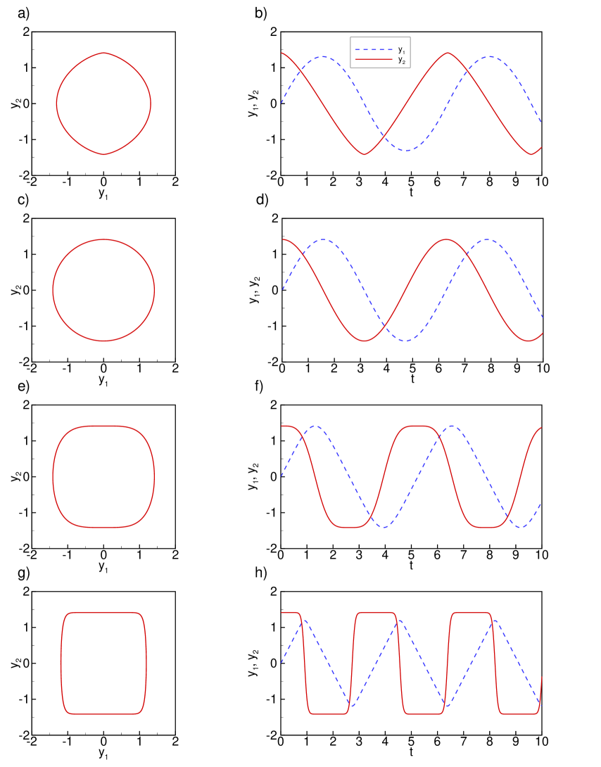
Figure 1: Normalized model for the oscillatory term: phase space (left panels) and time series (right panels) for a,b) $n=0.5$; c,d) $n=1$; e,f) $n=3$; and g,h) $n=15$. The continuous (resp. dashed) line is $y_{2}$ (resp. $y_{1}$).

as shown in the left panels of Figure 1. The original dynamics in ${\bf y}$ can be recovered using (48).

The closed orbit in phase space represents an oscillatory dynamics for any fixed $n>0$. For $n=1$, the curve given by (49) is a perfect circle with radius $\sqrt{2}$ corresponding to a linear harmonic oscillator (Figure 1c). For $n\neq 1$, the closed curve is a nonlinear generalization of the circle. As $n$ increases above $1$, $(\hat{y}_{1}^{2})^{n+1\over 2}$ becomes small for $|\hat{y}_{1}|<1$. From the condition (49), it follows that $|\hat{y}_{2}|$ remains almost constant near its maximum $\sqrt{2}$ for $|\hat{y}_{1}|<1$. Furthermore from (50), the range of $|\hat{y}_{1}|$ decreases monotonically to 1 as $n$ increases, while the range of $\hat{y}_{2}$ remains unchanged for any $n$. On the whole, the geometry of the closed orbit becomes closer and closer to a square as $n$ increases, as shown in Figures 1e and 1g.

The normalized dynamical model can be obtained by substituting (48) into (40). In addition, it can be decoupled into two independent first-order nonlinear ordinary differential equations (ODEs) using the condition (49):

$${d\over dt}\left(\begin{array}[]{c}\hat{y}_{1}\\ \hat{y}_{2}\end{array}\right)=\left(\begin{array}[]{c}\hat{y}_{2}\\ -\hat{y}_{1}|\hat{y}_{1}|^{n-1}\end{array}\right)=\left(\begin{array}[]{rll}{\rm sign}[\hat{y}_{2}]&\sqrt{2}&[1-{1\over n+1}(\hat{y}_{1}^{2})^{{n+1\over 2}}]^{{1\over 2}}\\ -{\rm sign}[\hat{y}_{1}]&(n+1)^{{n\over n+1}}&[1-{1\over 2}\hat{y}_{2}^{2}]^{{n\over n+1}}\end{array}\right)~{}.$$ (57)

Therefore, the normalized trajectory goes around the origin in a clockwise direction along the closed curve given by (49).

Given an initial condition $\hat{{\bf y}}_{0}$ satisfying (49), the two ODEs in (57) can be solved separately and provide the trajectory $\hat{{\bf y}}(\hat{t};\hat{{\bf y}}_{0},\hat{t}_{0})$. However, once $\hat{y}_{1}(\hat{t};\hat{{\bf y}}_{0},\hat{t}_{0})$ is solved using the top ODE, $\hat{y}_{2}(\hat{t};\hat{{\bf y}}_{0},\hat{t}_{0})$ can be algebraically computed using (49) without solving the bottom ODE for $\hat{y}_{2}$; and vice versa. The period of oscillation can be obtained by integrating one of the two ODEs over the range defined by (50).

For some special $n$’s, the normalized model has explicit analytical solutions. For $n=1$, corresponding to a harmonic oscillator, the solution is:

$$\hat{{\bf y}}(\hat{t};\hat{{\bf y}}_{0},\hat{t}_{0}) = \sqrt{2}(\sin(\hat{t}-\hat{t}_{0}+\theta),\cos(\hat{t}-\hat{t}_{0}+\theta))~{},$$ (58)

where the initial condition $\hat{{\bf y}}_{0}=\sqrt{2}(\sin\theta,\cos\theta)$ satisfies (49) for any real number $\theta$. Its period of oscillation is $2\pi$.

For $n=3$, the solution for $\hat{y}_{1}(\hat{t};\hat{{\bf y}}_{0},\hat{t}_{0})$ is [18]:

$$F\left(\arccos{\hat{y}_{1}(\hat{t})\over\hat{y}_{10}},{1\over\sqrt{2}}\right)=\hat{y}_{10}~{}(\hat{t}-{\hat{t}}_{0})~{},$$ (59)

where $\hat{y}_{10}\equiv\hat{y}_{1}(\hat{t}=\hat{t}_{0})$ and $\hat{y}_{2}(\hat{t}=\hat{t}_{0})=0$ and $F\left(u,k)\right)$ is the elliptic integral of the first kind defined by

$$F(u,k)=\int_{0}^{u}{dv\over\sqrt{1-k^{2}\sin^{2}v}}~{}.$$ (60)

The evolution of a trajectory with initial condition $\hat{{\bf y}}_{0}=(0,\sqrt{2})$ at $\hat{t}_{0}=0$ is shown in the right panels of Figure 1 as a function of $\hat{t}$. For $n=1$, the normalized variable $\hat{y}_{1}$ is preceded by its velocity $\hat{y}_{2}$ by a $\frac{\pi}{2}$-phase shift. As $n$ increases, the amplitude of the normalized velocity $|\hat{y}_{2}|$ becomes nearly constant about $\sqrt{2}$ for $|\hat{y}_{1}|<1$ [see Figures 1e and 1g as well as the discussion concerning the geometry of the normalized orbit given by (49)]. Accordingly, $\hat{y}_{1}$ evolves almost linearly in time with a constant velocity $\hat{y}_{2}=\pm\sqrt{2}$ for $|\hat{y}_{1}|<1$. Thus, time series of $\hat{y}_{1}$ and $\hat{y}_{2}$ respectively have saw-teeth and step-function shapes. The period of the oscillation becomes shorter as $n$ increases, because the velocity amplitude $|\hat{y}_{2}|$ remains closer and closer to its maximum as $n$ increases during each oscillation cycle.

5.1.3 Global dynamics

Having understood the template dynamics of the normalized model, we describe the global dynamics of the oscillatory element in the original model. Two parameters, $n$ and $\gamma$, are used to define the one-degree-of-freedom Hamiltonian system given by (40). From the normalization defined by (48) and the resulting system given by (57), we see that the exponent $n$ is the controlling parameter. The coefficient $\gamma$ contributes only for the scaling of $(y_{1},t)$.

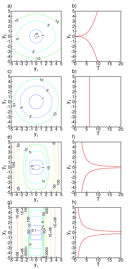
Figure 2: Phase portrait (left panels) and period $T$ of the oscillations (right panel) for the oscillatory term with $\gamma=1$ for all, so that $H=1$ corresponds to the normalized model (Figure 1): a,b) $n=0.5$; c,d) $n=1$; e,f) $n=3$; and g,h) $n=15$. The period of the oscillation is on the abscissa as a function of the maximum equal to $(2H)^{1\over 2}$ of $y_{2}$ on the ordinate.

For fixed $(n,\gamma)$, the phase portrait in ${\bf y}$ consists of a family of closed orbits parameterized by $H$. Each orbit has a unique $H$ and oscillates in the clockwise direction around the origin (left panels of Figure 2). Given the properties of the normalized orbit in Section 5.1.2, three main properties of individual orbit as function of $H$ follow.

First, $H$ measures the amplitude of oscillation. Each orbit in ${\bf y}$ ranges over:

$$y_{1}\in[-\left(\frac{(n+1)H}{\gamma}\right)^{{1\over n+1}},\left(\frac{(n+1)H}{\gamma}\right)^{{1\over n+1}}],~{}~{}y_{2}\in[-(2H)^{1\over 2},(2H)^{1\over 2}]~{}$$ (61)

from (48) and (50). The left panels of Figure 2 show the orbits in the ${\bf y}$ phase space as curves of constant $H$. The higher $H$ is, the larger is the amplitude of the oscillations.

Second, $H$ determines the geometry of the orbits, except for $n=1$ where all orbits are ellipses of the same aspect ratio $\gamma^{{1\over n+1}}$ (Figure 1c). For $n\neq 1$, we describe the geometry in terms of the deformation from the normalized curve (49) by comparing the two normalization coefficients for $y_{1}$ and $y_{2}$ in (61), i.e., $H^{1\over n+1}$ and $H^{1\over 2}$, respectively. These two coefficients also govern the range of the oscillation (48). For $n<1$, the two coefficients have the following relation: $H^{1\over n+1}<H^{1\over 2}<1$ for $H<1$, and $H^{1\over n+1}>H^{1\over 2}>1$ for $H>1$. Hence, an orbit with small amplitude ($H<1$) has a geometrical shape stretched along the vertical direction (Figure 2a), as deduced from the normalized closed curve (Figure 1a). This is because $y_{1}$ is reduced more than $y_{2}$. Similarly, an orbit with a large amplitude ($H>1$) has a geometrical shape stretched horizontally. For $n>1$, the relation is reversed: $1>H^{1\over n+1}>H^{1\over 2}$ for $H<1$, and $1<H^{1\over n+1}<H^{1\over 2}$ for $H>1$. Accordingly, orbits with small ($H<1$) or large ($H>1$) amplitudes respectively have horizontally or vertically stretched geometries compared with the normalized closed curve (Figure 2c,d).

Third, $H$ controls the speed of the oscillation, except for the harmonic oscillator case $n=1$ which has a constant period $2\pi/\sqrt{\gamma}$. For $n\neq 1$, the period of the oscillations is obtained using (48), (50) and (57):

$$T(H;n,\gamma) = C(n)~{}\gamma^{-1\over n+1}~{}H^{{1-n\over 2(n+1)}}~{},$$ (62)

where $C(n)$ is a positive number given by:

$$C(n)\equiv{4\over(n+1)^{{n\over n+1}}}\int_{0}^{\sqrt{2}}{d\hat{y}_{2}\over\left(1-{1\over 2}\hat{y}_{2}^{2}\right)^{{n\over n+1}}}~{}~{}.$$ (63)

Differentiating the expression of the period $T(H;n,\gamma)$ given by (62) with respect to $H$ gives:

$${\partial\over\partial H}T(H;n,\gamma) = {1-n\over 2(n+1)}~{}C(n)~{}\gamma^{-1\over n+1}~{}H^{-{3n+1\over 2(n+1)}}~{}~{}.$$ (64)

Therefore, ${\partial\over\partial H}T(H;n,\gamma)$ can be positive or negative depending on $n$. For $n<1$ where $\frac{\partial}{\partial H}T>0$, the period increases monotonically from $0$ to $\infty$ as $H$ increases. In contrast, for $n>1$, the period decreases monotonically from $\infty$ to $0$ as $H$ increases. The right panels of Figure 2 show the period of oscillation on the abscissa as function of the maximum amplitude reached by $y_{2}$ equal to $\sqrt{2H}$, given as a measure of the oscillation amplitude.

5.2 The trend term: singular behavior

We now consider the trend term and examine the nature of the singularity which manifests itself in “finite-time” in the behavior of the velocity $y_{2}$ and of the variable $y_{1}$. Motivated by the applications to concrete physical processes discussed in sections 2, 3 and 4, we focus on the case $\alpha>0$ and $m>1$.

5.2.1 Model

Keeping only the second term in the r.h.s. of (32) and re-writing it as a system of two-dimensional ODEs for the variable $y_{1}$ and its velocity $y_{2}$ give:

$$\frac{d}{dt}\left(\begin{array}[]{c}y_{1}\\ y_{2}\end{array}\right)=\left(\begin{array}[]{c}y_{2}\\ \alpha y_{2}|y_{2}|^{m-1}\end{array}\right)~{}.$$ (65)

In this system,

$$G({\bf y};m,\alpha)\equiv y_{1}-\left\{\begin{array}[]{ccl}{1\over\alpha(2-m)}&y_{2}|y_{2}|^{1-m}&~{}~{}~{}\mbox{for $m\neq 2$}~{},\\ {1\over\alpha}&{\rm sign}[y_{2}]\log|y_{2}|&~{}~{}~{}\mbox{for $m=2$}{}\end{array}\right.$$ (66)

is an invariant, i.e., ${d\over dt}G({\bf y};m,\alpha)=0$. This can be easily verified by differentiating (66) with respect to $t$ and then substituting in (65). Therefore, like $H({\bf y};n,\gamma)$ in the one-degree-of-freedom Hamiltonian system discussed in the previous section for the restoring term, a curve of constant $G({\bf y};m,\alpha)$ in the ${\bf y}$ phase space corresponds to an orbit governed by (65). A trajectory ${\bf y}(t;{\bf y}_{0},t_{0})$ going through ${\bf y}_{0}$ satisfies $G({\bf y}(t;{\bf y}_{0},t_{0});m,\alpha)=G({\bf y}_{0};m,\alpha)$ for any $t$.

5.2.2 Template dynamics in the normalized model

To describe the template dynamics of the trend term, we reduce the system (65) to a normalized model using the invariant $G$ (66). We define the following normalized variables denoted by $\tilde{\{\cdot\}}$:

$$\left(\begin{array}[]{c}y_{1}\\ y_{2}\\ t\end{array}\right)=\left(\begin{array}[]{clc}\alpha^{-1}&\tilde{y}_{1}&+~{}G\\ &\tilde{y}_{2}&\\ \alpha^{-1}&\tilde{t}&\end{array}\right)~{}.$$ (73)

Substituting (73) into (65) gives the normalized dynamical model:

$${d\over d\tilde{t}}\left(\begin{array}[]{l}\tilde{y}_{1}\\ \tilde{y}_{2}\end{array}\right)=\left(\begin{array}[]{c}\tilde{y}_{2}\\ \tilde{y}_{2}|\tilde{y}_{2}|^{m-1}\end{array}\right)~{}~{}.$$ (78)

Therefore, the normalized velocity $\tilde{y}_{2}$ undergoes an irreversible amplification if it starts from $|\tilde{y}_{2}|\neq 0$ and it pulls the variable $\tilde{y}_{1}$ along. The dividing point $\tilde{y}_{2}=0$ is a fixed point. Furthermore, substituting (73) into (66) gives an invariant condition for the normalized orbit:

$$\tilde{y}_{1}=\tilde{g}(\tilde{y}_{2})~{},$$ (79)

where

$$\tilde{g}(\tilde{y}_{2})=\left\{\begin{array}[]{cll}{1\over(2-m)}&\tilde{y}_{2}|\tilde{y}_{2}|^{1-m}&~{}~{}~{}\mbox{for $m\neq 2$}\\ {\rm sign}[\tilde{y}_{2}]&\log|\tilde{y}_{2}|&~{}~{}~{}\mbox{for $m=2$}{}\end{array}\right.~{}.$$ (82)

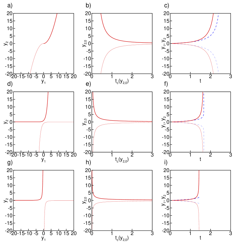
Figure 3: Normalized model for the singular term: phase space trajectories (left panels), critical time $t_{c}$ (center panels) as a function of the initial value $y_{2,0}$ and time series (right panels) for a–c) $m=1.5$; d–f) $m=2$; g–h) $m=2.5$. Thick and thin lines correspond to the pair of normalized orbits for $y_{2}>0$ and $y_{2}<0$, respectively, with initial condition $(y_{1,0},y_{2,0})=(0,\pm 0.6)$. The continuous (resp. dashed) line is $y_{2}$ (resp. $y_{1}$).

The left panels of Figure 3 show graphs of (79) for $m=1.5$, 2 and 2.5. Each graph consists of a pair of rotationally-symmetric orbits for $\tilde{y}_{2}>0$ and $\tilde{y}_{2}<0$ with the symmetry given by $\tilde{{\bf y}}\rightarrow-\tilde{{\bf y}}$. Through the normalization (73), all orbits in the original ${\bf y}$ phase space with $y_{2}>0$ collapse onto the single normalized orbit with $\tilde{y}_{2}>0$ in $\tilde{{\bf y}}$ phase space. Similarly, all orbits in the ${\bf y}$ phase space with $y_{2}<0$ collapse onto the single normalized orbit with $\tilde{y}_{2}<0$ in the $\tilde{{\bf y}}$ phase space. Using (78), the slope of the graph is:

$${d\tilde{y}_{2}\over d\tilde{y}_{1}}={d\tilde{y}_{2}\over d\tilde{t}}/{d\tilde{y}_{1}\over d\tilde{t}}=|\tilde{y}_{2}|^{m-1}~{}.$$ (83)

Integrating this equation retrieves the normalized invariant condition given by (79). For fixed $m$, the slope increases from 0 to $\infty$ as $|\tilde{y}_{2}|$ increases. The higher $m$ is, the faster the slope increases.

The geometry of (the pair of) symmetric normalized orbit(s) depends on $m$ significantly (Figure 3). This is due to a qualitatively different behavior of $\tilde{y}_{1}=\tilde{g}(\tilde{y}_{2})$ as $\tilde{y}_{2}$ approaches towards either end of the normalized orbit. For $\tilde{y}_{2}>0$,

$$\tilde{y}_{1}=\tilde{g}(\tilde{y}_{2})\in\left\{\begin{array}[]{ll}(0,\infty)&\mbox{for $1<m<2$}\\ (-\infty,\infty)&\mbox{for $m=2$}\\ (-\infty,0)&\mbox{for $m>2$}\end{array}\right.,~{}\tilde{y}_{2}\in(0,\infty)~{}.$$ (87)

In other words, the normalized model undergoes a bifurcation at $m=2$. Precisely for $m=2$, $\tilde{g}(\tilde{y}_{2})$ spans the whole interval $(-\infty,\infty)$ and thus interpolates between the cases for $m<2$ and $m>2$ for which only one-half of the interval is covered by the dynamics.

Accordingly, the dynamical behavior of the normalized trajectory changes qualitatively when $1<m<2$, $m=2$ or $m>2$. Any initial condition $\tilde{{\bf y}}_{0}\equiv(\tilde{y}_{1,0},\tilde{y}_{2,0})$ of the normalized trajectory $\tilde{{\bf y}}(\tilde{t};\tilde{{\bf y}}_{0},\tilde{t}_{0})$ must satisfy (79), i.e., $\tilde{y}_{1,0}=\tilde{g}(\tilde{y}_{2,0})$. Using this initial condition, (78) can be solved analytically:

$$\tilde{y}_{1}(\tilde{t};\tilde{{\bf y}}_{0},\tilde{t}_{0}) = \tilde{g}(\tilde{y}_{2,0})+{\rm sign}[\tilde{y}_{2,0}]~{}$$ (90)

$$\times\left\{\begin{array}[]{ll}(m-1)^{{m-2\over m-1}}~{}{1\over 2-m}~{}[(\tilde{t}_{c}(\tilde{y}_{2,0})-\tilde{t})^{{m-2\over m-1}}-(\tilde{t}_{c}(\tilde{y}_{2,0})-\tilde{t}_{0})^{{m-2\over m-1}}]&\mbox{for $m\neq 2$}\\ \log\left({\tilde{t}_{c}-\tilde{t}_{0}\over\tilde{t}_{c}(\tilde{y}_{2,0})-\tilde{t}}\right)&\mbox{for $m=2$}\end{array}\right.~{},$$

$$\tilde{y}_{2}(\tilde{t};\tilde{{\bf y}}_{0},\tilde{t}_{0}) = {\rm sign}[\tilde{y}_{2,0}]~{}(m-1)^{-{1\over m-1}}~{}(\tilde{t}_{c}(\tilde{y}_{2,0})-\tilde{t})^{-{1\over m-1}}~{}.$$ (91)

The solution is valid only for a semi-infinite time interval $\tilde{t}\in(-\infty,\tilde{t}_{c}(\tilde{y}_{2,0}))$ up to the normalized “critical time:”

$$\tilde{t}_{c}(\tilde{y}_{2,0})=\tilde{t}_{0}+{1\over m-1}|\tilde{y}_{2,0}|^{1-m},$$ (92)

for any arbitrary $\tilde{t}_{0}$. The center panels of Figure 3 shows $\tilde{t}_{c}$ on the abscissa as a function of $\tilde{y}_{2,0}$ on the ordinate with $\tilde{t}_{0}=0$. The solution becomes singular as $\tilde{y}_{2}$ approaches $\pm\infty$, and no solution exists for $\tilde{t}>\tilde{t}_{c}(\tilde{y}_{2,0})$.

This is the “finite-time” singular behavior for the velocity amplitude $|\tilde{y}_{2}|$, which occurs for any $m>1$. It is driven by the nonlinear positive feedback of the trend term producing a faster than exponential growth rate, leading to a infinite growth of $|\tilde{y}_{2}|$ in finite time. For a fixed $m$, the initial normalized velocity $\tilde{y}_{2,0}$ solely determines the behavior of the trajectory given by (91) and (92), as a consequence of the fact that the dynamics (78) is solely determined by $\tilde{{\bf y}}_{2}$. The evolution of $\tilde{{\bf y}}_{2}(\tilde{t};\tilde{{\bf y}}_{0},\tilde{t}_{0})$ in time with a pair of initial conditions $\tilde{{\bf y}}_{0}=(0,\pm 0.6)$ at $\tilde{t}_{0}=0$ is shown in the right panels of Figure 3.

We now examine separately the behavior for forward $(\tilde{t}>\tilde{t}_{0})$ and backward $(\tilde{t}<\tilde{t}_{0})$ time intervals. Using the parity symmetry, we focus on the dynamics described by the normalized orbit with $\tilde{y}_{2,0}>0$. Similar results hold for $\tilde{y}_{2,0}<0$ using $\tilde{{\bf y}}\rightarrow-\tilde{{\bf y}}$.

Over a forward finite time interval $\tilde{t}\in[\tilde{t}_{0},\tilde{t}_{c}(\tilde{y}_{2,0}))$ up to $\tilde{t}_{c}(\tilde{y}_{2,0})$, the normalized trajectory with initial condition $\tilde{y}_{2,0}>0$ ranges over:

$$\tilde{y}_{1}\in\left\{\begin{array}[]{ll}\left[\tilde{g}(\tilde{y}_{2,0}),\infty)\right.&\mbox{for $1<m\leq 2$}\\ \left[0,\tilde{g}(\tilde{y}_{2,0}))\right.&\mbox{for $m>2$}\end{array}\right.~{},~{}~{}\tilde{y}_{2}\in[\tilde{y}_{2,0},\infty)~{},$$ (95)

as shown in the left and right panels of Figure 3. During this finite time interval up to $\tilde{t}_{0}(\tilde{y}_{2,0})$, $\tilde{y}_{2}$ grows from $\tilde{y}_{2,0}$ to $\infty$. For $1<m<2$, $\tilde{y}_{1}$ also blows up to infinity, dragged along by $\tilde{y}_{2}$. On the contrary for $m>2$, $\tilde{y}_{1}$ culminates at a finite value, given by $\tilde{g}(\tilde{y}_{2,0})$. This finiteness of $\tilde{y}_{1}$ occurs only for $m>2$ for which the relative growth rate of $\tilde{y}_{2}$ compared to $\tilde{y}_{1}$ also becomes singular, as given by the slope of the graph $\frac{d\tilde{y}_{2}}{d\tilde{y}_{1}}=\frac{d\tilde{y}_{2}}{d\tilde{t}}/\frac{d\tilde{y}_{1}}{d\tilde{t}}$ in (83). The finite final value $\tilde{g}(\tilde{y}_{2,0})$ of $\tilde{y}_{1}$ can be observed in Figure 3g using the graph of the normalized orbit (79) by replacing $(\tilde{y}_{1},\tilde{y}_{2})$ by $(\tilde{g}(\tilde{y}_{2,0}),\tilde{y}_{2,0})$.

In contrast, over a backward semi-infinite time interval $\tilde{t}<\tilde{t}_{0}$, the normalized trajectory ranges over:

$$\tilde{y}_{1}\in\left\{\begin{array}[]{rl}(0,\tilde{g}(\tilde{y}_{2,0})]&\mbox{for $1<m<2$}\\ (-\infty,\tilde{g}(\tilde{y}_{2,0})]&\mbox{for $m\geq 2$}\end{array}\right.,~{}~{}~{}\tilde{y}_{2}\in(0,\tilde{y}_{2,0}]~{}~{}.$$ (98)

The normalized velocity $\tilde{y}_{2}$ hence shrinks to $0$, resulting in a finite increment equal $\tilde{y}_{2,0}$ over the whole time interval. For $1<m<2$, the increment $\tilde{g}(\tilde{y}_{2,0})$ in $\tilde{y}_{1}$ is also finite. On the contrary for $m>2$, the increment in $\tilde{y}_{1}$ is infinite because the relative growth rate given by slope $\frac{d\tilde{y}_{1}}{d\tilde{y}_{2}}$ diverges for $\tilde{y}_{2}\ll 1$.

5.2.3 Global dynamics

We now derive the global dynamics from the template dynamics of the normalized model constructed with the trend term. Two parameters, $m$ and $\alpha$, are used to define the two-dimensional representation of the trend term given by (65) and (66). For fixed $(m,\alpha)$, the model has the parity symmetry: ${\bf y}\rightarrow-{\bf y}$. We refer to the pair of symmetric orbits corresponding to the graph of $G({\bf y};m,\alpha)=0$ as the “reference orbits”. From the normalization (73), we see that the dynamics along the pair of reference orbits is related to the dynamics along the normalized orbits (79)–(98) through scaling of $(\tilde{y}_{1},\tilde{t})$ by $\alpha^{-1}$. We also see that all orbits in the ${\bf y}$ phase space collapse onto the corresponding reference orbit through linear translations in the $y_{1}$ phase space given by the distance $G({\bf y};m,\alpha)$. Therefore, the dynamics along any orbit is exactly the same as the one along the corresponding reference orbit, except for a translation in the $y_{1}$ phase space.

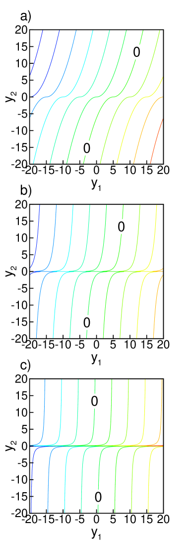
Figure 4: Phase portrait for the singular term with $\alpha=1$ for all cases, so that the reference orbits with $G=0$ (labeled by 0) corresponds to the normalized model (Figure 3): a) $m=1.5$; b) $m=2$; c) $m=2.5$.

Accordingly, the phase portrait for any $m$ consists in a pair of symmetric families of open orbits. Each family is parameterized by $G$ (Figure 4) where the reference orbits are labeled by “0” [see also the left panels of Figure 3 for comparison with the normalized orbits]. On $y_{2}=0$, the dynamics is at rest. Therefore, the ${\bf y}$ phase space can be divided into dynamically distinct regions as follows.

Definition 5.2.1

Singular basins $B_{\rm sing}^{+}$ and $B_{\rm sing}^{-}$ and boundary $b_{\rm sing}$
  We define a pair of singular basins:

$$B_{\rm sing}^{+} \equiv \{{\bf y}|~{}y_{2}>0,~{}\mbox{where }{d\over dt}y_{2}>0\}$$

$$B_{\rm sing}^{-} \equiv \{{\bf y}|~{}y_{2}<0,~{}\mbox{where }{d\over dt}y_{2}<0\}~{}~{}.$$ (99)

The boundary which separate the two basins is defined by:

$$b_{\rm sing} \equiv \{{\bf y}|y_{2}=0,~{}\mbox{where }{d\over dt}y_{2}=0\}~{}.$$ (100)

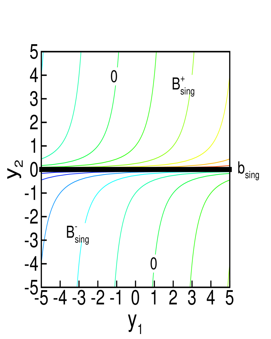
Figure 5: Two singular basins and the boundary between them for the singular term with $(m,\alpha)=(2.5,1)$ (see also Figures 3g and 4c for the normalized model) in the ${\bf y}$ phase space. The reference orbits are labeled by 0.

Any point ${\bf y}_{0}$ in the phase space belongs to either one of $B_{\rm sing}^{+}$, $B_{\rm sing}^{-}$ or $b_{\rm sing}$, as shown in figure 5.

For any $m>1$, the individual trajectory satisfies the following.

Corollary 5.2.2

  Consider a trajectory ${\bf y}(t;{\bf y}_{0},t_{0})$ with initial condition ${\bf y}_{0}=(y_{1,0},y_{2,0})$ at time $t_{0}$. If it starts in $B_{\rm sing}^{\pm}$, then it will remain within the basin without never leaving it. It will reach the corresponding finite-time singularity, i.e.,

$$\mbox{if ${\bf y}_{0}\in B_{\rm sing}^{\pm}$},\qquad\mbox{then ${\bf y}(t;{\bf y}_{0},t_{0})\in B_{\rm sing}^{\pm}$,}$$

$$\qquad\mbox{for $t\in(-\infty,t_{c}(y_{2,0}))$ ~{}~{}~{} with $y_{2}(-\infty;{\bf y}_{0},t_{0})=\pm 0$ ~{} and ~{}$y_{2}(t_{c}(y_{2,0});{\bf y}_{0},t_{0})=\pm\infty$}.$$ (101)

The critical time $t_{c}(y_{2,0})={\alpha}^{-1}\tilde{t}_{c}(\tilde{y}_{2,0})$ is a function of the initial velocity $y_{2,0}$ only. In the case where ${\bf y}(t;{\bf y}_{0},t_{0})$ starts on $b_{\rm sing}$, it will remain on the boundary basin without never leaving it for a bi-infinite time interval, i.e.,

$$\mbox{if ${\bf y}_{0}\in b_{\rm sing}$}, {\bf y}(t;{\bf y}_{0},t_{0})={\bf y}_{0}\in b_{\rm sing},\qquad\mbox{for $t\in(-\infty,-\infty)$}~{}.$$ then

Definition 5.2.3

Source strips $S_{\rm sing}^{+}$ and $S_{\rm sing}^{-}$
  Right next to the boundary $b_{\rm sing}$ in each basin $B_{\rm sing}^{\pm}$, we define a thin vertical strip of constant width:

$$S_{\rm sing}^{\pm} \equiv \{{\bf y}\in B_{\rm sing}^{\pm}~{}|~{}|y_{2}|<1,~{}\mbox{where $|\frac{d}{dt}y_{2}|=|y_{2}|^{m+1}\ll 1$}\}~{},$$ (102)

where ${\bf y}(t;{\bf y}_{0},t_{0})$ moves away from $b_{\rm sing}$ extremely slowly. Once it leaves $S_{\rm sing}^{\pm}$, it then reaches very quickly the finite-time singularity. For any ${\bf y}_{0}$, integrating with backward time, any ${\bf y}(t;{\bf y}_{0},t_{0})$ will eventually enter $S_{\rm sing}^{\pm}$. Therefore, $S_{\rm sing}^{\pm}$ can be considered as source regions of the finite-time singularity.

However, the qualitative behavior of each individual orbit in each singular basin depends on the specific value of the exponent $m$, as discussed in Section 5.2.2.

6 Overall dynamics: Fundamental characteristics

6.1 Normalized model

We now consider the overall dynamics obtained by combining the restoring and trend terms which have been analyzed separately in Section 5. We use the following normalized variables:

$$\left(\begin{array}[]{l}\bar{y}_{1}\\ \bar{y}_{2}\\ \bar{t}\\ \bar{\gamma}\end{array}\right)=\left(\begin{array}[]{lc}\alpha&y_{1}\\ &y_{2}\\ \alpha&t\\ \alpha^{-(n+1)}&\gamma\end{array}\right)~{}~{}$$ (111)

to minimize the number of parameters by removing the coefficient $\alpha$ of the positive feedback trend term. For simplicity in the notations, we drop the bar $\bar{\{\cdot\}}$ from here on. Then, the overall dynamical systems is written as:

$${d\over dt}\left(\begin{array}[]{l}y_{1}\\ y_{2}\end{array}\right) = \left(\begin{array}[]{l}y_{2}\\ \dot{y}_{2~{}{\rm osc}}+\dot{y}_{2~{}{\rm sing}}\end{array}\right)$$ (116)

where

$$\dot{y}_{2~{}{\rm osc}} = -\gamma y_{1}|y_{1}|^{n-1}$$ (117)

$$\dot{y}_{2~{}{\rm sing}} = y_{2}|y_{2}|^{m}~{},$$ (118)

are the oscillatory ($\dot{y}_{2~{}{\rm osc}}$) and singular ($\dot{y}_{2~{}{\rm sing}}$) source terms for the equation on the acceleration $\frac{d}{dt}y_{2}$ (inertia) of $y_{1}$, as discussed separately in Section 5.

6.2 Heuristic discussion: Time evolution

The interplay between the two previously documented regimes of oscillatory and singular behaviors results into oscillatory finite-time singularities. As a result of the nonlinearity of the restoring term ($n>1$), the oscillations have local frequencies modulated by the amplitude of $y_{1}$. We stress again that the solution $y_{1}(t;{\bf y}_{0},t_{0})$ is controlled by the initial condition $({\bf y}_{0},t_{0})$. In this heuristic discussion, we shall use the simplified notation $y_{1}$ for $y_{1}(t;{\bf y}_{0},t_{0})$.

A naive and approximate way to understanding the origin of the frequency modulation is that the expression $-\left(\gamma~{}|y_{1}|^{n-1}\right)~{}y_{1}$ defines a local frequency proportional to $\sqrt{\gamma}|y_{1}|^{n-1\over 2}$: the local frequency of the oscillations increases with the amplitude of $y_{1}$. It turns out that this naive guess is correct, as shown by the expressions (167) with (168) of section 7.4.4. We thus expect the local frequency to accelerate as the singular time $t_{c}$ is approached. if the amplitude $|y_{1}(t)|$ grows like $(t^{*}-t)^{-z}$ (see the derivation leading to (173), then the local period, corresponding to the distance between successive peaks of the oscillations, will be modulated and proportional to $\left(t_{c}-t\right)^{-{z(n-1)\over 2}}$.

6.2.1 Case $m=1$

We study

$${d^{2}y_{1}\over dt^{2}}=\alpha{dy_{1}\over dt}-\gamma~{}{\rm sign}[y_{1}]|y_{1}|^{n}~{},$$ (119)

and re-introduce the parameter $\alpha$ to allow us investigating the effect of its sign.

The interplay between the l.h.s. and the first term of the r.h.s. of (119) leads to an exponentially growing trend ${dy_{1}\over dt}$ and thus an exponentially growing typical amplitude of $y_{1}(t)$. If $y_{1}(t)\sim e^{\alpha t}$, both ${d^{2}y_{1}\over dt^{2}}$ and ${dy_{1}\over dt}$ are of the same order while the reversal term is of order $y_{1}^{n}\sim-e^{n\alpha t}$, showing that the oscillations will be a dominating feature of the solution. This is indeed what we observe in figure 6 which shows the solution of (119) for the parameters $\alpha=1$, $m=1,n=3$, $\gamma=-10$, $y_{1}(t=0)=1$ and $y_{2}(t=0)=5$. The amplitude of $y_{1}(t)$ grows exponentially and the accelerating oscillations have their frequency increasing also approximately exponentially with time, in agreement with our qualitative argument.

6.2.2 Case $m>1$

Case $\alpha>0$ and $1<m<2$: $|y_{1}(t\to t_{c})|=|y_{2}(t\to t_{c})|\to+\infty$

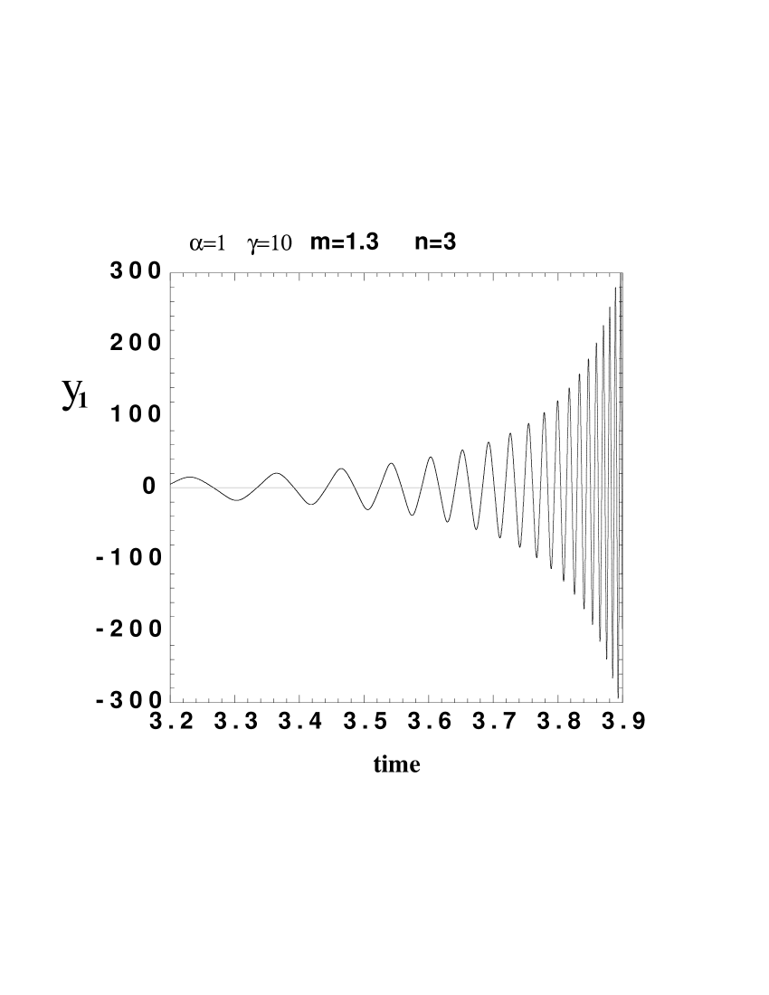
Figure 7: Solution of (32) for the parameters $m=1.3$, $n=3$, $\alpha=1$, $\gamma=10$ and $y_{20}\equiv dy_{1}/dt|_{t=0}=1$. The envelop of $y_{1}(t)$ grows faster than exponential and approximately as $(t_{c}-t)^{-1.5}$ where $t_{c}\approx 4$.

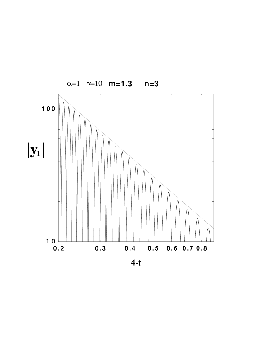
Figure 8: Same data as in figure 7: the absolute value $|y_{1}(t)|$ is shown as a function of $t_{c}-t$ where $t_{c}=4$ in log-log coordinates, such that a linear envelop qualifies the power law divergence $(t_{c}-t)^{-1.5}$. The slope of the line is $-1.5$. Notice also that the oscillations are approximately equidistant in the variable $\ln(t_{c}-t)$ resembling a log-periodic behavior of accelerating oscillations on the approach to the singularity.

In this regime, $y_{1}(t)$ diverges on the approach of $t_{c}$ as an inverse power of $(t_{c}-t)$. The accelerating oscillations are shown in figures 7 and 8 for the parameters $m=1.3$, $n=3$, $\alpha=1$, $\gamma=10$, $y_{1}(t=0)=1$ and $y_{2}(t=0)=1$. We observe that the envelop of $y_{1}(t)$ grows faster than exponential and approximately as $(t_{c}-t)^{-1.5}$ where $t_{c}\approx 4$. In figure 8, $|y_{1}(t)|$ is represented as a function of $t_{c}-t$ where $t_{c}=4$. A double logarithmic coordinate is used such that a linear envelop qualifies the power law divergence. The slope of the line shown on the figure gives the exponent $-1.5$ which is significantly different from the prediction $-(2-m)/(m-1)=-2.33$ given by (91) on the basis of the trend term only, i.e., by neglecting the reversal oscillatory term. The reversal term has the effect of “renormalizing” the exponent downward. Notice also that the oscillations are approximately equidistant in the variable $\ln(t_{c}-t)$ resembling a log-periodic behavior of accelerating oscillations on the approach to the singularity. Here, we shall not dwell more on this regime which gives divergent $y_{1}$ and $y_{2}$ and concentrate rather on the rest of the paper (except for the next subsection) on the case $m\geq 2$.

Case $\alpha<0$ and $1<m<2$: power law decay

Equation (32) obeys the symmetry of scale invariance for special choices of the two exponents $m$ and $n$. Consider indeed the following transformation where $t$ is changed into $\lambda t^{\prime}$ and $y_{1}$ is changed into $\mu y_{1}^{\prime}$. Inserting these two changes of variables in (32) gives

$$\mu\lambda^{2}{d^{2}y_{1}^{\prime}\over dt^{\prime 2}}=\alpha{\mu^{m}\over\lambda^{m}}{dy_{1}^{\prime}\over dt^{\prime}}|{dy_{1}^{\prime}\over dt^{\prime}}|^{m-1}-\gamma\mu^{n}y_{1}^{\prime}|y_{1}^{\prime}|^{n-1}~{}.$$ (120)

We see that (120) is the same equation as (32) if

$$n=1+2{m-1\over 2-m}~{},$$ (121)

for which we also have

$$\mu=\lambda^{-{2\over n-1}}~{}.$$ (122)

The condition (121) holds for instance with $m=1.5$ and $n=3$. When the relationship (121) is true, the two equations (120) and (32) are identical and their solutions are thus also identical for the same initial conditions: $y_{1}(t)=y_{1}^{\prime}(t^{\prime})$. This implies that the solution of (32) obeys the following exact renormalization group equation in the limit of large times when the effect of the initial conditions have been damped out:

$$y_{1}(t)={1\over\mu}y_{1}(\lambda t)~{},$$ (123)

where $\lambda$ is an arbitrary positive number and $\mu(\lambda)$ is given by (122). Looking for a solution of the form $y_{1}\sim t^{\beta}$, we get

$$\beta=-{2\over n-1}~{}.$$ (124)

This exact solution, describing the asymptotic regime $t\to+\infty$, corresponds to the decaying regime obtained when $\alpha$ is negative and will not be further explored in the sequel which focus on the singular case $\alpha>0$ and $m>1$.

Case $m>2$: $|y_{1}(t\to t_{c})|<+\infty$ and $|y_{2}(t\to t_{c})|\to+\infty$

In this case with $\alpha>0$, the solution of (65) gives a singularity in finite time with divergence as ${dy_{1}\over dt}\sim(t_{c}-t)^{-1/(m-1)}$. Since $1/(m-1)<1$, $y_{1}(t)$ remains finite with a singularity in finite time of the type

$$y_{1}(t)\sim y_{c}-A(t_{c}-t)^{m-2\over m-1}$$ (125)

with infinite slope but finite value $Y$ at the critical time $t_{c}$ since $(m-2)/(m-1)>0$.

The consequence is that there can be only at most a finite number of oscillations. Indeed, since $y_{1}(t)$ goes to a finite constant, it becomes negligible compared to its first and second derivatives which both diverge close to $t_{c}$. Therefore, the two first terms in (32) dominate close to the singularity and the oscillations, which are controlled by the last term, finally disappear and the solution becomes a pure power law (125) asymptotically close to $t_{c}$.

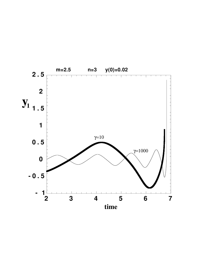
Figure 9: Solutions obtained from a numerical integration of (32) with $m=2.5$ yielding the exponent ${m-2\over m-1}=1/3$ for the terminal singular behavior of $y_{1}\sim y_{1c}-A(t_{c}-t)^{m-2\over m-1}$ close to $t_{c}$, for $n=3$, $\alpha=1$ and initial value $y_{10}=0.02$ and derivative $y_{20}={dy_{1}\over dt}|_{0}=-0.3$ and for two amplitudes $\gamma=10$ and $\gamma=1000$ of the reversal term.

Figure 9 shows the solutions obtained from a numerical integration of (32) with $m=2.5$ yielding the exponent ${m-2\over m-1}=1/3$, for $n=3$ and initial value $y_{1}(t=0)=0.02$ and derivative ${dy_{1}\over dt}|_{t=0}\equiv y_{2,0}=-0.3$ for two amplitudes $\gamma=10$ and $\gamma=1000$ of the reversal term. Notice the existence of a finite number of oscillations and the upward divergence of the slope. As expected, the stronger the reversal term, the larger is the number of oscillations before the pure power law singularity sets in. The number of oscillations is very strongly controlled by the initial value of the slope ${dy_{1}\over dt}|_{0}$. For $m=2.5,n=3$ and initial value $y_{1}(0)=0.02$ with $\gamma=10$, for instance increasing the slope in absolute value to ${dy_{1}\over dt}|_{0}=-0.7$ gives a single dip followed by a power law acceleration. Intuitively, the number of oscillations is controlled by the proximity of this initial starting point to the unstable fixed point $(0,0)$, the closest to it, the larger is the number of oscillations.

These properties are formalized into a systematic dynamical system approach in section 7.

6.3 Heuristic discussion: Phase space

6.3.1 Properties in the phase space

Having understood the dynamics of the two elements separately (Section 5) and with the qualitative insight provided by the previous examples, we pose the natural question:

• Can oscillatory and/or singular dynamics persist in the presence of their interaction?

The direct numerical integration of the equations of motion in Section 6.2 suggests a positive answer. In the next section 7, we address this question in a formal way and construct a precise phase portrait of the overall dynamics for given $(n,m,\gamma)$. Here we articulate the problem by identifying fundamental properties of a trajectory ${\bf y}(t;{\bf y}_{0},t_{0})$ in the phase space. First, we recall that the full dynamical equation is invariant under parity symmetry in phase space: $({\bf y},\frac{d}{dt}{\bf y})\to(-{\bf y},-\frac{d}{dt}{\bf y})$. The origin ${\bf y}=(0,0)$ is a fixed point:

$${d\over dt}{\bf y}\big{|}_{(0,0)}=0~{}~{}.$$ (126)

More precisely, it is a clockwise unstable nonlinear focus in the ${\bf y}$ phase space because the flow is divergent everywhere:

$$\nabla\cdot{d\over dt}{\bf y}={\partial\over\partial y_{2}}\dot{y}_{2{\rm osc}}=m|y_{2}|^{m-1}\geq 0~{}~{}.$$ (127)

Therefore, starting extremely near the origin $|{\bf y}_{0}|\ll 1$, ${\bf y}(t;{\bf y}_{0},t_{0})$ undergoes a clockwise oscillation with increasing amplitude.

Next, we examine the properties of the oscillations. When only the oscillatory term $\dot{y}_{2{\rm osc}}$ is present (i.e., $\dot{y}_{2{\rm sing}}=0$), Section 5.1.3 showed that the amplitude and the period of the oscillations can be determined by $H$ alone. When the singular term $\dot{y}_{2{\rm sing}}$ is added, $H$ is no longer conserved along any trajectory but increases instead:

$${d\over dt}H({\bf y};n,m,\gamma) = \left({d\over dt}y_{1}\right)~{}\dot{y}_{2{\rm sing}}=|y_{2}|^{m+1}\geq 0~{}.$$ (128)

The growth rate of $H$ also increases as $H$ increases, because a higher $H$ corresponds to a wider range of $y_{2}$ during an oscillation cycle, as seen from (61). The higher $H$ becomes, the more effective is the impact of $\dot{y}_{2{\rm sing}}$, especially once $|y_{2}(t;{\bf y}_{0},t_{0})|$ reaches ${\cal O}(1)$. The region where $|y_{2}(t;{\bf y}_{0},t_{0})|<1$ corresponds to the source strips $S_{\rm sing}^{\pm}$ (Definition 5.2.3) for the case with only the singular term $\dot{y}_{2{\rm sing}}$.

Remark 6.3.1

For $n>1$, ${\bf y}(t;{\bf y}_{0},t_{0})$ has the following characteristics:

1. From (64), the frequency of oscillation increases from $0$ to $\infty$ as $H$ increases. As a consequence, for $|y_{2}|\ll 1$ where ${d\over dt}H$ is very small, ${\bf y}(t;{\bf y}_{0},t_{0})$ undergoes extremely slowly divergent oscillation with increasing frequency.

2. From (61), the amplitude of the oscillations monotonically grows as $H$ grows to $\infty$ at an increasing rate. As a consequence, $|{\bf y}(t;{\bf y}_{0},t_{0})|$ eventually diverges to $\infty$.

3. From (128), ${\bf y}(t;{\bf y}_{0},t_{0})$ starting from any ${\bf y}_{0}$ approaches the origin backward in time.

4. Therefore, $|{\bf y}(t;{\bf y}_{0},t_{0})|$ starting from any ${\bf y}_{0}$ connects the origin $|{\bf y}(t;{\bf y}_{0},t_{0})|\rightarrow 0$ in backward time and infinity $|{\bf y}(t;{\bf y}_{0},t_{0})|\rightarrow\infty$ in forward time.

We now formulate mathematically the notion of an oscillation for the overall dynamics. When ${\bf y}(t;{\bf y}_{0},t_{0})$ undergoes a sequence of oscillation cycle in the ${\bf y}$ phase space (see for example Figure 1), $y_{1}$ and $y_{2}$ change their direction of motion in succession.

Definition 6.3.2

Turn of a trajectory
  We say that ${\bf y}(t;{\bf y}_{0},t_{0})$ makes a turn at $t=t^{\prime}$ if the variable $y_{1}$ changes its direction of motion at $t=t^{\prime}$, i.e.,

$${d\over dt}y_{1}\big{|}_{{\bf y}(t^{\prime};{\bf y}_{0},t_{0})}=y_{2}=0.$$ (129)

Each complete oscillation cycle requires two turns of ${\bf y}(t;{\bf y}_{0},t_{0})$. During a time interval between two adjacent turns, $y_{2}$ changes directions (i.e., it achieves $\frac{d}{dt}y_{2}=0$) if the oscillation is around the origin ${\bf y}=(0,0)$; see for example Figure 1.

Definition 6.3.3

Zero velocity curves $F^{(1)}$ and $F^{(2)}$
  We define the two zero-velocity curves in the phase space with respect to $y_{1}$ and $y_{2}$:

$$F^{(1)} \equiv \{{\bf y}\big{|}~{}~{}{d\over dt}y_{1}=0~{},~{}~{}\mbox{i.e., $y_{2}=0$}\}~{},$$ (130)

$$F^{(2)} \equiv \{{\bf y}\big{|}~{}~{}{d\over dt}y_{2}=0~{},~{}~{}\mbox{i.e., $\gamma y_{1}|y_{1}|^{n-1}=y_{2}|y_{2}|^{m-1}$}\}~{}.$$ (131)

$F^{(1)}$ is nothing but the $y_{1}$-axis. On the curve $F^{(2)}$, $y_{1}$ can be expressed as a monotonic function of $y_{2}$:

$$y_{2}\equiv f^{(2)}(y_{1})=\gamma^{{1\over m}}~{}y_{1}|y_{1}|^{{n\over m}-1}~{},$$ (132)

where $(y_{1},f^{(2)}(y_{1}))$ is on $F^{(2)}$. An alternative way for obtaining (130) and (131) is to use the slope of the trajectory ${\bf y}(t;{\bf y}_{0},t_{0})$ in phase space:

$${dy_{2}\over dy_{1}}\big{|}_{{\bf y}(t;{\bf y}_{0},t_{0})} = {dy_{2}\over dt}/{dy_{1}\over dt}\big{|}_{{\bf y}(t;{\bf y}_{0},t_{0})}=\frac{-\gamma y_{1}|y_{1}|^{n-1}+y_{2}|y_{2}|}{y_{2}}~{},$$ (133)

where ${dy_{2}\over dy_{1}}=\pm\infty$ results in $F^{(1)}$ and ${dy_{2}\over dy_{1}}=0$ gives $F^{(2)}$.

Corollary 6.3.4

Complete oscillation cycle
  Staring from a point on $F^{(1)}$ where ${\bf y}(t;{\bf y}_{0},t_{0})$ makes a turn (i.e., ${\bf y}_{0}\in F^{(1)}$), one complete oscillation cycle requires a set of four conditions to be satisfied in sequence: [$\frac{d}{dt}y_{1}=0$ $\mapsto$ $\frac{d}{dt}y_{2}=0$ $\mapsto$ $\frac{d}{dt}y_{1}=0$ $\mapsto$ $\frac{d}{dt}y_{2}=0$]. Accordingly, in phase space, ${\bf y}(t;{\bf y}_{0},t_{0})$ cuts across [$F^{(1)}$ $\mapsto$ $F^{(2)}$ $\mapsto$ $F^{(1)}$ $\mapsto$ $F^{(2)}$] in succession.

Corollary 6.3.5

Transition to non-oscillatory motion
  If ${\bf y}(t;{\bf y}_{0},t_{0})$ ceases to reach $F^{(1)}$ or $F^{(2)}$, then it can no longer oscillate around the origin.

6.3.2 Schematic dynamics in phase space

Having Corollaries 6.3.4 and 6.3.5 in hands, we rephrase the question in Section 6.3.1 into more specific ones:

• Under what conditions and how far does the clockwise oscillatory motion owing to $\dot{y}_{2{\rm osc}}$ persist away from the origin?

• Under what conditions does the finite-time singular behavior persist, and the two singular basins resulting from $\dot{y}_{2{\rm sing}}$ exist?

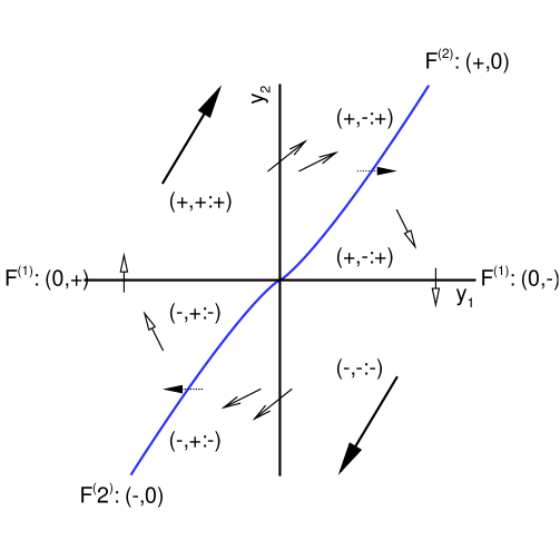
Figure 10: Schematic velocity field ${d\over dt}{\bf y}$ indicated by arrows. The phase space is divided into six regions by $F^{(1)}$, $F^{(2)}$ and $y_{1}=0$. The effect of the reversions and trend terms in each region are shown by the sign of $\dot{y}_{2{\rm osc}}$ and $\dot{y}_{2{\rm sing}}$ in $({d\over dt}y_{1},\dot{y}_{2{\rm osc}}:\dot{y}_{2{\rm sing}})$. $\dot{y}_{2{\rm osc}}$ and $\dot{y}_{2{\rm sing}}$ may enhance each other (long thick arrows); $\dot{y}_{2{\rm sing}}$ dominates $\dot{y}_{2{\rm osc}}$ (plain arrowhead); $\dot{y}_{2{\rm osc}}$ dominates $\dot{y}_{2{\rm sing}}$ (hollow arrowhead). On $F^{(2)}$, they balance (dotted line).

For an intuitive grasp of issues associated with these questions, we schematically summarize in Figure 10 the dynamical properties along a trajectory ${\bf y}(t;{\bf y}_{0},t_{0})$ due respectively to $\dot{y}_{2{\rm osc}}$ and $\dot{y}_{2{\rm sing}}$. The total velocity vector $(dy_{1}/dt,dy_{2}/dt)$ is indicated by the arrows. The sign of the two contributing terms $\dot{y}_{2{\rm osc}}$ and $\dot{y}_{2{\rm sing}}$ are given in the triplet $({d\over dt}y_{1},\dot{y}_{2{\rm osc}}:\dot{y}_{2{\rm sing}})$. The two terms $\dot{y}_{2{\rm osc}}$ and $\dot{y}_{2{\rm sing}}$ can enhance or oppose each other depending on their relative signs.

Furthermore, we make the following observations.

Remark 6.3.6

1. The phase space is divided into six domains by $F^{(1)}$, $F^{(2)}$ and $y_{1}=0$. On $F^{(1)}$ and $F^{(2)}$, the components of the velocity vector, ${d\over dt}y_{1}$ and ${d\over dt}y_{2}$, respectively change their sign. On $y_{1}=0$ and $F^{(1)}$, ${d\over dt}y_{1}$ and $\dot{y}_{2{\rm sing}}$ change sign.

2. In the second or fourth quadrant ($y_{1}y_{2}<0$) defined by $F^{(1)}$ and $y_{1}=0$, both $\dot{y}_{2{\rm sing}}$ and $\dot{y}_{2{\rm osc}}$ have the same sign and hence so does $\frac{d}{dt}y_{2}$. In Figure 10, it is indicated by long thick arrow with the velocity triplet $({d\over dt}y_{1},\dot{y}_{2{\rm osc}}:\dot{y}_{2{\rm sing}})=(-,-:-)$ in the second quadrant or $(+,+:+)$ in the fourth quadrant. It can be thought that $\dot{y}_{2{\rm osc}}$ enhances $\dot{y}_{2{\rm sing}}$ in a way that ${\bf y}(t;{\bf y}_{0},t_{0})$ flows towards one of the two ($+$ or $-$) singular directions in $y_{2}$ from the following reason.

   • Because $\dot{y}_{2{\rm sing}}$ and $\dot{y}_{2{\rm osc}}$ have the same sign, $|{d\over dt}y_{2}|=|\dot{y}_{2{\rm sing}}|+|\dot{y}_{2{\rm osc}}|$ is larger than $|\dot{y}_{2{\rm sing}}|$. Therefore, if ${\bf y}(t;{\bf y}_{0},t_{0})$ remains in the second or fourth quadrant without ever leaving, it must be driven to a finite-time singularity with the same sign as in the case where only $\dot{y}_{2{\rm sing}}$ operates, but at a faster rate. Therefore, two singular basins inevitably exist:

     1. In the fourth quadrant where $y_{2}>0$ and $y_{1}<0$: $y_{2}\to+\infty$ with ${d\over dt}y_{2}>0$ and ${d\over dt}y_{1}>0$,

     2. In the second quadrant where $y_{2}<0$ and $y_{1}>0$: $y_{2}\to-\infty$ with ${d\over dt}y_{2}<0$ and ${d\over dt}y_{1}<0$.

     These two basins are the generalization of the two basins $B_{\rm sing}^{\pm}$ defined previously for $\dot{y}_{2{\rm sing}}$ only (Definition 5.2.1). This partially answers Q2 above.

   • The only way for ${\bf y}(t;{\bf y}_{0},t_{0})$ to escape from the singular behavior is to leave the second or fourth quadrant respectively for the third or first quadrant by cutting $y_{1}=0$ while keeping the sign of $y_{2}$.

3. In the first or third quadrant ($y_{1}y_{2}>0$) defined by $y_{1}=0$ and $F^{(1)}$ with $F^{(2)}$ inside, $\dot{y}_{2{\rm osc}}$ and $\dot{y}_{2{\rm sing}}$ have opposite signs and the total velocity vector cannot be determined unambiguously as indicated by the velocity triplet $({d\over dt}y_{1},\dot{y}_{2{\rm osc}}:\dot{y}_{2{\rm sing}})=(+,-:+)$ in the first quadrant or $(-,+:-)$ in the third quadrant. When ${\bf y}(t;{\bf y}_{0},t_{0})$ enters into the first of third quadrant according to clockwise motion around the origin, it respectively comes from the fourth or second quadrant where $\dot{y}_{2{\rm sing}}$ enhances $\dot{y}_{2{\rm sing}}$ as indicated by plain arrowheads in Figure 10. Therefore, $\dot{y}_{2{\rm sing}}$ is dominant first. Then, the effect of $\dot{y}_{2{\rm osc}}$ gradually kicks in as $|y_{1}|$ increases towards $F^{(2)}$ where $\dot{y}_{2{\rm osc}}$ balances $\dot{y}_{2{\rm sing}}$ as indicated by dotted line in Figure 10.

   • If $\dot{y}_{2{\rm sing}}$ remains dominant and ${\bf y}(t;{\bf y}_{0},t_{0})$ never reaches $F^{(2)}$, then ${d\over dt}y_{2}$ does not change sign and $y_{2}$ keeps growing. Eventually, $\dot{y}_{2{\rm sing}}$ may completely dominate $\dot{y}_{2{\rm osc}}$, and ${\bf y}(t;{\bf y}_{0},t_{0})$ moves quickly towards the terminal singularity,

     1. In the first quadrant where $y_{1}>0$ and $y_{2}>0$ above $F^{(2)}$: $y_{2}\to+\infty$ with ${d\over dt}y_{2}>0$ and ${d\over dt}y_{1}>0$,

     2. In the third quadrant where $y_{1}<0$ and $y_{2}<0$ below $F^{(2)}$: $y_{2}\to-\infty$ with ${d\over dt}y_{2}<0$ and ${d\over dt}y_{1}<0$.

     The sign of $y_{2}$ towards the singularity is consistent for all quadrants.

   • If ${\bf y}(t;{\bf y},t_{0})$ reaches $F^{(2)}$, $\dot{y}_{2{\rm osc}}$ overcomes $\dot{y}_{2{\rm sing}}$ and $\frac{d}{dt}y_{2}$ changes sign as indicated by hollow arrowhead in Figure 10. Eventually ${\bf y}(t;{\bf y},t_{0})$ has to exit the quadrant by passing $F^{(1)}$. It follows that, if ${\bf y}(t;{\bf y},t_{0})$ reaches $F^{(2)}$, then it also reaches $F^{(1)}$ and makes a turn of an oscillation (Definition 6.3.2).

In summary, the following two conditions sequentially determine whether or not ${\bf y}(t;{\bf y}_{0},t_{0})$ can make another turn starting from a turning point ${\bf y}_{0}\in F^{(1)}$:

1. In the fourth or second quadrant: whether or not it reaches $y_{1}=0$.

2. In the first or third quadrant if it reaches $y_{1}=0$: whether or not it reaches $F^{(2)}$.

For fixed $(n,m,\gamma)$, the global dynamics can be completely described by the phase portrait because this is a system of two-dimensional autonomous ODEs. However, this geometrical structure of the phase portrait may bifurcate as the value of the exponents $n$ and $m$ vary (Section 5.1 and 5.2). In the following section, we will examine the structure of the global dynamics when both elements have high nonlinearity, i.e., $n>1$ and $m>2$.

7 Overall dynamics for $n>1$ and $m>2$ with $\alpha>0$: $|y_{1}(t\to t_{c})|<+\infty$ (except for isolated initial conditions) and $|y_{2}(t\to t_{c})|=+\infty$

Recall from Section 5.1 for the sub-dynamical system with only the oscillatory element that the case $n>1$ corresponds to highly nonlinear oscillations with a monotonically decreasing period as the amplitude of the oscillations increases (Figure 2). From Section 5.2 for the sub-dynamical system with only the singular element, the case $m>2$ corresponds to finite-time singularity with finite increment in $y_{1}$ and infinite increment in $y_{2}$ (Figure 4). Furthermore, Section 6.3 on the phase space of the full dynamical system showed the following results:

1. any trajectory ${\bf y}(t;{\bf y}_{0},t_{0})$ starting away from the origin connects the origin in backward time and $|y_{2}|\rightarrow\infty$ in forward time;

2. the oscillations may persist especially near the origin;

3. the finite-time singular behavior should persist;

4. the $F^{(2)}$-curve is critical in determining whether or not a trajectory transits from oscillatory to singular behavior.

As we demonstrate below, the most striking dynamical feature for the case $n>1$ and $m>2$ is the finite-time oscillatory singularity. In Section 7.1, we heuristically describe the global dynamics by identifying the boundaries and basins in the phase space using two examples. The mathematical definitions of the boundaries and basins are given in Section 7.2. Using the template maps, we describe the global dynamics of the boundaries in Section 7.3.1 and the basins in Section 7.3.2. Finally, we study the scale-invariant properties associated with the finite-time oscillatory singularity in Section 7.4.

7.1 Phase space description

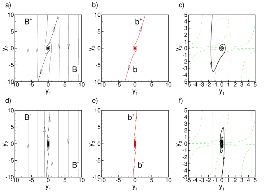
Figure 11: Global dynamics in the phase space with $(n,m)=(3,2.5)$ for $\gamma=10$ (a-c) and $\gamma=1000$ (d–f): a,d) phase portrait as a collection of trajectories; b,e) singular boundary $b^{\pm}$, and c,f) a trajectory starting ${\bf y}_{0}=(-0.06,0)$ with contours of $H$ (dotted lines) and $G$ (dashed lines) for reference (see also Figures 2 and 4, respectively). Arrows along trajectories indicate the forward direction of time.

Two examples of phase portraits are shown in Figure 11 as a collection of trajectories with $(n,m)=(3,2.5)$ for $\gamma=10$ (Figure 11a–c) and $\gamma=1000$ (Figure 11d–f), where arrows along the individual trajectories indicate the direction of forward time. We observe in both examples that there are two basins (labeled by $B^{+}$ and $B^{-}$) in the phase space. The superscript of individual basins correspond to the sign of the terminal direction $\frac{d}{dt}y_{2}$ as $|y_{2}|\rightarrow\infty$. The boundary between the basins is kinematically defined by the special trajectories spirally out of the origin to reach $|y_{1}|\rightarrow\infty$ as well as $|y_{2}|\rightarrow\infty$. Any other trajectories result in a finite terminal value of $y_{1}$ as $|y_{2}|\rightarrow\infty$. These boundary trajectories are singled out in Figures 11b and e (labeled by $b^{+}$ and $b^{-}$). A typical trajectory ${\bf y}(t;{\bf y}_{0},t_{0})$ starting from ${\bf y}_{0}=(-0.06,0)$ are also shown in Figures 11c and f.

These phase portraits confirm that oscillations indeed persist and are confined near the origin about $|{\bf y}|<1$ and hence $H<1$ from (41). The amplitude of the oscillations continuously grows along ${\bf y}(t;{\bf y}_{0},t_{0})$ in forward time as seen from (128). For $|y_{2}|\ll 1$ starting near the origin $|{\bf y}_{0}|\ll 1$, ${\bf y}(t;{\bf y}_{0},t_{0})$ is nearly vertical because of $|\frac{d}{dt}y_{2}|\gg|\frac{d}{dt}y_{1}|$ and follows a constant $H$-curve closely (Section 5.1.3, see also Figure 2). For $|y_{2}|$ no more much smaller than $1$, $H$ increases more efficiently by growing further in $y_{2}$ as observed in Figures 11c and f. The period of the oscillations decreases continuously, because $\frac{d}{dt}T(H;n,\gamma)=\frac{\partial T}{\partial H}\frac{dH}{dt}\leq 0$ along ${\bf y}(t;{\bf y}_{0},t_{0})$ for $n>1$.

Once the oscillation reaches $|{\bf y}|\approx 1$ and hence $H\approx 1$, the singular element $\dot{y}_{2{\rm sing}}$ works on $\frac{d}{dt}y_{2}$ more effectively. As a result, ${\bf y}(t;{\bf y}_{0},t_{0})$ starts to grow rapidly, especially when it is moving vertically in the phase space.

Recall also that closed $H$ contours for $H>1$ are stretched out vertically for $n>1$ (Section 5.1.3). Therefore, the oscillatory element $\dot{y}_{2{\rm osc}}$ can enhance or suppress the singular behavior of ${\bf y}(t;{\bf y}_{0},t_{0})$ significantly when it moves vertically. Such stretching effect of $H$ is more prominent for larger $\gamma$ (compare Figures 11c to f).

For $|y_{2}|>1$, the dynamics is extremely singular in the second and fourth quadrants where $\dot{y}_{2{\rm osc}}$ enhances $\dot{y}_{2{\rm sing}}$ (Remark 6.3.6). The terminal increment of $y_{1}$ is nearly zero as $y_{2}$ approaches singularity in finite time as indicated by the almost vertical trajectories.

In the first and third quadrants where $\frac{d}{dt}y_{2}$ changes sign with respect to $\dot{y}_{2{\rm osc}}$ on $F^{(2)}$, the boundaries $b^{+}$ and $b^{-}$ divide the phase space into $B^{+}$ and $B^{-}$. Any trajectory starting near $b^{+}$ and $b^{-}$ with $|y_{2}|>1$ accelerates extremely fast into $B^{+}$ or $B^{-}$, indicating that the dynamics is extremely sensitive near $b^{+}$ and $b^{-}$ for $|y_{2}|>1$. Any trajectory that moves away from $b^{+}$ or $b^{-}$ for $|y_{2}|>1$ does so almost vertically due to the stretched structure of $H$ for $H>1$. Near vertical trajectories away from $b^{+}$ or $b^{-}$ indicate that increment of $y_{1}$ is finite in the first and third quadrants like in the second and fourth quadrants.

7.2 Singular basins and boundary

When the dynamics has only the trend element (Section 5.2), there exist two singular basins $B_{\rm sing}^{+}$ and $B_{\rm sing}^{-}$ separated by a boundary $b_{\rm sing}$ determined by a collection of stagnation points where the velocity is identically zero (Definition 5.2.1). In the full dynamical system, we define the two boundaries $b^{+}$ and $b^{-}$ kinematically as observed in Figure 11. The definition of the two basins $B^{+}$ and $B^{-}$ follow in a natural way. For simplicity and economy in notation, we use $\pm$ and $\mp$ to represent two distinct cases by choosing them consistently in order. For example, by “$\pm A$ with $\mp B$ for $\pm C$,” we mean: i) “$+A$ with $-B$ for $+C$,” and ii) “$-A$ with $+B$ for $-C$.” Use of $\pm$ and $\mp$ is possible because the full dynamical equation is invariant under parity symmetry.

Definition 7.2.1

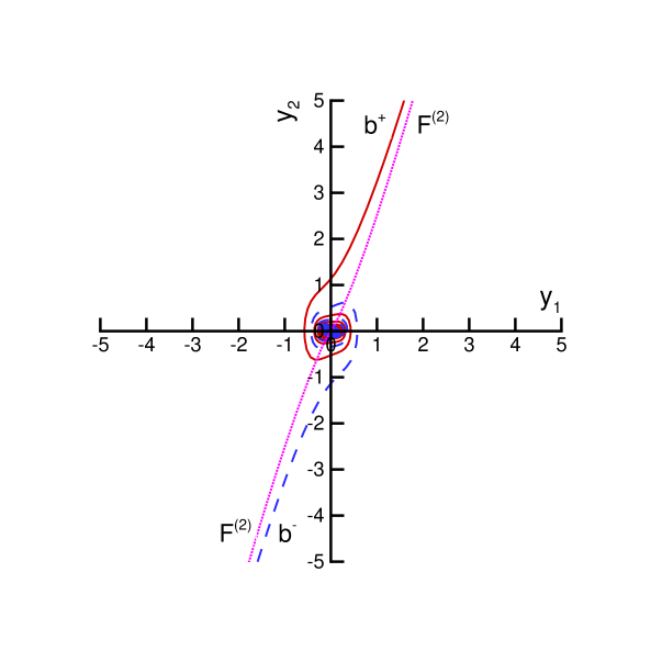
Figure 12: Geometrical relation between $b^{\pm}$ and $F^{(2)}$ for $(n,m)=(3,2.5)$ and $\gamma=10$ as in Fig. 11.

Boundaries $b^{+}$ and $b^{-}$. [see Definition 5.2.1]
  We define the boundary $b^{\pm}$ by the special trajectories that connect the origin ${\bf y}=(0,0)$ to $(+\infty,+\infty)$ and to $(-\infty,-\infty)$ (see Figures 11 and 12). Any trajectory ${\bf y}(t;{\bf y}_{0},t_{0})$ starting on ${\bf y}_{0}\in b^{\pm}$ will remain on it in forward and backward time:

$$\mbox{if ${\bf y}_{0}\in b^{\pm}$},\qquad {\bf y}(t;{\bf y}_{0},t_{0})\in b^{\pm}\qquad\qquad\mbox{for $t\in(-\infty,\infty)$}$$ then (134)

with $${\bf y}(-\infty;{\bf y}_{0},t_{0})=(0,0),\qquad{\bf y}(\infty;{\bf y}_{0},t_{0})=(\pm\infty,\pm\infty).$$

Corollary 7.2.2

Asymptotic behavior of $b^{+}$ and $b^{-}$.
  As $|y_{2}|\to+\infty$, $b^{\pm}$ asymptotically approaches $F^{(2)}$ where ${d\over dt}y_{2}=0$ (Figure 12). A trajectory ${\bf y}(t;{\bf y}_{0},t_{0})$ with ${\bf y}_{0}\in b^{\pm}$ has the following properties.

• It can never reach $F^{(2)}$, because if it does, it will have to exit the region where $y_{1}y_{2}>0$ and this leads to a contradiction (Remark 6.3.6, Item 3),

• It must stay near $F^{(2)}$ so that the near zero velocity ${d\over dt}y_{2}\sim 0$ keeps the trajectory from growing rapidly to a singularity in a finite time. This also leads to a contradiction (Theorem 7.2.1).

Because the boundary is kinematically defined, we have the following theorem for the basins.

Theorem 7.2.3

Basins $B^{+}$ and $B^{-}$. [see Definition 5.2.1]
  There exist two distinct basins $B^{+}$ and $B^{-}$ kinematically divided by $b^{+}$ and $b^{-}$. Any trajectory ${\bf y}(t;{\bf y}_{0},t_{0})$ with ${\bf y}_{0}\in B^{\pm}$ will remain within it and reaches a finite-time singularity, i.e.,

$$\mbox{if ${\bf y}_{0}\in B^{\pm}$},\qquad {\bf y}(t;{\bf y}_{0},t_{0})\in B^{\pm}\qquad\qquad\mbox{for $t\in(-\infty,t_{c}({\bf y}_{0})+t_{0})$}$$ then (135)

with $$\lim_{t\to-\infty}{\bf y}(t;{\bf y}_{0},t_{0})=(0,0),$$

$$\lim_{t\to t_{c}({\bf y}_{0})+t_{0}}{\bf y}(t;{\bf y}_{0},t_{0})={\bf y}_{c}({\bf y}_{0}),\qquad{\bf y}_{c}({\bf y}_{0})=(y_{1c}({\bf y}_{0}),\pm\infty).$$

where ${\bf y}_{c}({\bf y}_{0})$ and $t_{c}({\bf y}_{0})$ are the finite-time singularity and finite-time singular interval. They depend only on the initial condition ${\bf y}_{0}$ because the system is autonomous. Any other trajectory not starting in $B^{\pm}$ initially can never enter into $B^{\pm}$ by cutting across $b^{\pm}$ due to the uniqueness of the solution.

As seen on the two examples in Figure 11, in the presence of both the trend and the reversal terms, the oscillatory behavior persists near the origin. Technically, whether or not the oscillations persist depends on the competition between the oscillatory and singular elements with respect to the time-scales. In Section 7.4, we will examine this issue in details using scaling arguments. Here, we proceed with our discussion assuming that such oscillations do exist, as observed in figure 11.

Remark 7.2.4

For $|{\bf y}|\gg 1$ outside of the oscillatory region, two basins $B^{\pm}$ are clearly visible (see Figures 11 and 12): $B^{+}$ lies “above” $b^{+}$, and $B^{-}$ lies “below” $b^{-}$. This description is carried into the oscillatory region using the direction of the flow as follows.

1. $B^{+}$ basin: “above” the boundaries $b^{\pm}$, i.e., to the left of $b^{+}$ and to the right of $b^{-}$ with respect to the forward direction in the flow (see also in Figure 11). Any trajectory ${\bf y}(t;{\bf y}_{0},t_{0})$ with ${\bf y}_{0}\in B^{+}$ goes to $y_{2}(t_{c};{\bf y}_{0},t_{0})\to+\infty$.

2. $B^{-}$ basin: “below” the boundaries $b^{\pm}$, i.e., to the left of $b^{-}$ and to the right of $b^{+}$ with respect to the forward direction in the flow. Any ${\bf y}(t;{\bf y}_{0},t_{0})$ with ${\bf y}_{0}\in B^{-}$ goes to $y_{2}(t_{c};{\bf y}_{0},t_{0})\to-\infty$.

In other words, $b^{\pm}$ lies to the right of $B^{\pm}$ with respect to the forward direction of the flow.

7.3 Global dynamics

7.3.1 Dynamical properties along the boundaries

The structure of the phase space is completely governed by the boundary $b^{\pm}$. Therefore, we first study the dynamical properties along $b^{\pm}$.

Definition 7.3.1

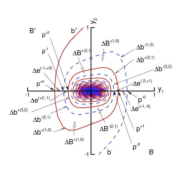
Figure 13: Geometry of boundaries $b^{\pm}$ and basins $B^{\pm}$ for $(n,m)=(3,2.5)$ and $\gamma=10$. See text for details.

Exit turn ${\bf p}^{\pm 0}$ as the intersection of $b^{\pm}$ with the $y_{1}$-axis
  We define a point ${\bf p}^{\pm 0}$ as the out-most intersection of $b^{\pm}$ with the $y_{1}$-axis as shown in Figure 13. Therefore, ${\bf y}(t;{\bf p}^{\pm 0},t_{0})$ makes no further turn for $t>t_{0}$ (Definition 6.3.2). We call ${\bf p}^{\pm 0}$ the exit turn point. The transition from oscillatory to singular behaviors occurs at ${\bf p}^{\pm 0}$.

Definition 7.3.2

Reference trajectory ${\bf y}^{\pm}(t)$, turn points ${\bf p}^{\pm k}$ and exit time $t^{\pm k}$
  We define ${\bf y}^{\pm}(t)$ as the reference trajectory on $b^{\pm}$ which goes through the exit turn point ${\bf p}^{\pm 0}$ at time $t=0$, i.e.,

$${\bf y}^{\pm}(t)\equiv{\bf y}(t;{\bf p}^{\pm 0},0)~{}.$$ (136)

In backward time, ${\bf y}^{\pm}(t)$ makes a turn by intersecting the $y_{1}$-axis (Definition 6.3.2). At time $t^{\pm k}(<0)$, ${\bf y}^{\pm}(t)$ makes the $k$-th (backward) turn:

$${\bf y}^{\pm}(t^{\pm k})={\bf p}^{\pm k},$$ (137)

where

$${\bf p}^{\pm k}\equiv(y_{1}^{\pm k},0)~{}\in b^{\pm}~{}~{}$$ (138)

is defined as the $k$-th turn points. It is located at an intersection of $b^{\pm}$ and $y_{1}$ axis (Figure 13). By construction, a trajectory ${\bf y}(t;{\bf p}^{\pm k},t^{\pm k})$ is on the reference trajectory. Starting from ${\bf p}^{\pm k}$, the trajectory makes $k$ turns before reaching the exit turn point ${\bf p}^{\pm 0}$ at time 0 after a time interval $-t^{\pm k}(>0)$. It does not make any more turns for $t>0$. We call $t^{\pm k}(<0)$ the $k$-th exit time.

Definition 7.3.3

Template map for the dynamics associated with ${\bf p}^{\pm k}$ along $b^{\pm}$
  We define the template map of the dynamics along each boundary $b^{\pm}$ using the sequence of turn points ${\bf p}^{\pm k}$:

$$\ldots\triangleright{\bf p}^{\pm k+1} \triangleright {\bf p}^{\pm k}\triangleright\ldots\triangleright{\bf p}^{\pm 0}~{}.$$ (139)

By construction, there is no other turn points between any ${\bf p}^{\pm k+1}$ and ${\bf p}^{\pm k}$ along $b^{\pm}$.

Remark 7.3.4

As shown in Figure 13,

1. Along $b^{\pm}$ in forward time, the turn points ${\bf p}^{\pm k}$ jump between $y_{1}>0$ and $y_{1}<0$ as ${\bf y}^{\pm}(t)$ oscillates around the origin:

   • along $b^{+}$: $y_{1}^{+(2l)}<0$ and $y_{1}^{+(2l+1)}>0$,

   • along $b^{-}$: $y_{1}^{-(2l+1)}<0$ and $y_{1}^{-(2l)}>0$.

2. On the $y_{1}$-axis, the turn points alternate between $b^{+}$ and $b^{-}$:

   $$y_{1}^{+0}~{}<~{}y_{1}^{-1}~{}<~{}y_{1}^{+2}~{}<~{}y_{1}^{-3}<~{}y_{1}^{+4}~{}<~{}\ldots~{}<~{}y_{1}^{-4}~{}<~{}y_{1}^{+3}~{}<~{}y_{1}^{-2}~{}<~{}y_{1}^{+1~{}}<~{}y_{1}^{-0}~{},$$ (140)

Remark 7.3.5

Three main dynamical properties associated with ${\bf p}^{\pm k}$ are as follows:

1. the alternating signs of $y_{1}^{\pm k}$, i.e., $(-1)^{k}y_{1}^{+k}<0$ along $b^{+}$ and $(-1)^{k}y_{1}^{-k}>0$ along $b^{-}$ (Corollary 7.3.4);

2. the finite number of turns $N_{turns}=k$ in forward time before exiting from the oscillatory region (Corollary 7.3.2);

3. the exit time $t^{\pm k}$ (Definition 7.3.2).

These properties are summarized in Table 1 (see also Figure 13) using the template map ($\triangleright$) to show the dynamics in forward time.

${\bf p}^{\pm k}$	$\ldots$	$\triangleright$	${\bf p}^{\pm(k+1)}$	$\triangleright$	${\bf p}^{\pm(k)}$	$\triangleright$	$\ldots$	$\triangleright$	${\bf p}^{\pm 1}$	$\triangleright$	${\bf p}^{\pm 0}$	$\triangleright$	[$(\pm\infty,\pm\infty)$]
sign of $y_{1}^{\pm k}$	$\ldots$	$\triangleright$	$(-1)^{(k+1)}\mp$	$\triangleright$	$(-1)^{k}\mp$	$\triangleright$	$\ldots$	$\triangleright$	$(-1)^{1}\mp$	$\triangleright$	$\mp$	($\triangleright$	[$\pm$])
$N_{turn}$	$\ldots$	$\triangleright$	$k+1$	$\triangleright$	$k$	$\triangleright$	$\ldots$	$\triangleright$	$1$	$\triangleright$	$0$
$t^{\pm k}$	$\ldots$	$\triangleright$	$t^{\pm(k+1)}$	$\triangleright$	$t^{\pm k}$	$\triangleright$	$\ldots$	$\triangleright$	$t^{\pm 1}$	$\triangleright$	$0$

Table 1: Dynamical properties associated with the template map of ${\bf p}^{\pm k}$ along the singular boundary $b^{\pm}$ (Remarks 7.3.5).

We now present the dynamical properties of arbitrary trajectories along $b^{\pm}$ using the template map. To do so, we partition $b^{\pm}$ into boundary segments bounded by the points ${\bf p}^{\pm(k)}$.

Definition 7.3.6

Boundary segment
  We define the boundary segment $\triangle b^{\pm(k+1,k)}$ of $b^{\pm}$ to be a segment between two adjacent turn points ${\bf p}^{\pm(k+1)}$ and ${\bf p}^{\pm k}$ (both exclusive) :

$$\triangle b^{\pm(k+1,k)}\equiv\{{\bf y}^{\pm}(t),~{}\mbox{for $t\in(t^{\pm k+1},t^{\pm k})$}\}~{}~{},$$ (141)

(see also Figure 13). The symbol “$($” and “$)$” in the superscript are used to indicate that both the left and right endpoints are outside of the interval.

Remark 7.3.7

1. The semi-infinite unions of the boundary segments together with the semi-infinite unions of turn points forms the boundary:

   $$b^{\pm}=\cup_{k=0}^{\infty}\triangle b^{\pm(k+1,k)}~{}\cup~{}\triangle b^{\pm(\cdot,0)}~{}\cup_{k=0}^{\infty}{\bf p}^{\pm k}~{}~{},$$ (142)

   where

   $$\triangle b^{\pm(0,\cdot)}\equiv\{{\bf y}={\bf y}^{\pm}(t),~{}\mbox{for $t\geq 0$}\}~{}.$$ (143)

2. By construction, ${\bf y}^{\pm}(t)$ makes no turn over any boundary segment $\triangle b^{\pm(k+1,k)}$.

The complete description of the dynamical properties along $b^{\pm}$ follows.

Corollary 7.3.8

Dynamical properties of a trajectory ${\bf y}(t;{\bf y}_{0},t_{0})$ on $b^{\pm}$
  Let us consider a trajectory ${\bf y}(t;{\bf y}_{0},t_{0})$ on $b^{\pm}$ starting from a point ${\bf y}_{0}$ in the boundary segment ${\bf y}_{0}\in\triangle b^{\pm(k+1,k)}$ at an arbitrary time $t_{0}$. It reaches the turn point ${\bf p}^{\pm k}$ in forward time after a time interval $-\triangle t_{b}^{\pm(k+1,k)}(>0)$ without making any turn, where

$$t^{\pm(k+1)}-t^{\pm k}<\triangle t_{b}^{\pm(k+1,k)}<0~{},$$ (144)

because $t^{\pm k}-t^{\pm(k+1)}$ is the total time of flight over $\triangle b^{\pm(k+1,k)}$. Accordingly, ${\bf y}(t;{\bf y}_{0},t_{0})$ with ${\bf y}_{0}\in\triangle b^{\pm(k+1,k)}$ has the same dynamical properties as ${\bf y}^{\pm}(t)$ starting from ${\bf p}^{\pm k}$ (Table 1), except that the exit time is extended from $t^{\pm k}$ to $t^{\pm k}+\triangle t_{b}^{\pm(k+1,k)}$. It can also be expressed using the reference trajectory

$${\bf y}(t;{\bf y}_{0},t_{0})={\bf y}^{\pm}(t-t_{0}+t^{\pm k}+\triangle t_{b}^{\pm(k+1,k)})~{},$$ (145)

because ${\bf y}(t_{0};{\bf y}_{0},t_{0})={\bf y}^{\pm}(t^{\pm k}+\triangle t_{b}^{\pm(k+1,k)})$.

7.3.2 Dynamical properties in the basins

As the dynamical properties along the boundaries $b^{\pm}$ can be described by a template map of turn points ${\bf p}^{\pm k}$, the dynamical properties in the basin $B^{\pm}$ can also described by a template map of turn segments as follows.

Definition 7.3.9

Turn segments $\triangle e^{(\pm(k+1),\mp k)}$
  Any trajectory ${\bf y}(t;{\bf y}_{0},t_{0})$ can make a turn only on the $y_{1}$-axis (Definition 6.3.2). We define a turn segment $\triangle e^{(\pm(k+1),\mp k)}$ as being bounded by two adjacent turn points ${\bf p}^{\pm(k+1)}$ and ${\bf p}^{\mp k}$ on the $y_{1}$-axis (Figure 13):

• for $y_{1}<0$ $\triangle e^{(+0,-\infty)}$ $\equiv\{{\bf y}~{}|~{}-\infty<y_{1}<y_{1}^{+0}<0,y_{2}=0\}$$\in B^{+}$;
    $\triangle e^{(-(2l+1),+(2l))}$ $\equiv\{{\bf y}~{}|~{}p^{+(2l)}<y_{1}<p^{-(2l+1)}<0,y_{2}=0\}$$\in B^{-}$;
    $\triangle e^{(+(2l),-(2l-1))}$ $\equiv\{{\bf y}~{}|~{}p^{-(2l-1)}<y_{1}<p^{+(2l)}<0,~{}y_{2}=0\}$$\in B^{+}$;

• for $y_{1}>0$ $\triangle e^{(-(2l),+(2l-1))}$ $\equiv\{{\bf y}~{}|~{}0<p^{-(2l)}<y_{1}<p^{+(2l-1)},~{}y_{2}=0\}$$\in B^{-}$;
    $\triangle e^{(+(2l+1),-(2l))}$ $\equiv\{{\bf y}~{}|~{}0<p^{+(2l+1)}<y_{1}<p^{-(2l)},~{}y_{2}=0\}$$\in B^{+}$;
    $\triangle e^{(-0,+\infty)}$ $\equiv\{{\bf y}~{}|~{}0<p^{-0}<y_{1}<\infty,y_{2}=0\}$$\in B^{-}$.

The notational convention for the superscript of the turn segment $\triangle e^{(\pm(k+1),\mp k)}$ is that the left and right indices, $\pm(k+1)$ and $\mp k$, respectively correspond to the superscript of the turn points, ${\bf p}^{\pm(k+1)}$ and ${\bf p}^{\mp k}$, which are respectively at the left and right ends of the segment with respect to forward direction of the flow (see Remark 7.2.4). The symbols “(” and “)” in the superscript mean that these intersection points are not included in the segment.

Remark 7.3.10

In comparison with Remark 7.3.4:

1. Along the flow in forward time, the turn segments jump between $y_{1}<0$ and $y_{1}>0$ as a trajectory in $B^{\pm}$ oscillates around the origin:

   • in $B^{+}$: $y_{1}<0$ for $\triangle e^{(+(2l+1),-(2l))}$ and $y_{1}>0$ for $\triangle e^{(+(2l),-(2l-1)}$;

   • in $B^{-}$: $y_{1}<0$ for $\triangle e^{(-(2l),+(2l-1))}$ and $y_{1}>0$ for $\triangle e^{(-(2l+1),+(2l)}$;

2. Moreover, the $y_{1}$-axis consists of the union of all intersection points and segments;

   $$y_{1} = \triangle e^{(+0,-\infty)}\cup{\bf p}^{+0}\cup\triangle e^{(-1,+0)}\cup{\bf p}^{-1}\cup\triangle e^{(+2,-1)}\cup{\bf p}^{+2}\cup$$-axis (146)

   $$~{}~{}~{}\ldots\cup(0,0)\cup\ldots\cup{\bf p}^{-2}\cup\triangle e^{(-2,+1)}\cup\triangle e^{(+1,-0)}\cup{\bf p}^{-0}\cup\triangle e^{(-0,+\infty)}~{}.$$

   Note that the superscript of $\triangle e^{(\pm(k+1),\mp k)}$ for $y_{1}<0$ is not in sequence with the subscript of ${\bf p}^{\pm(k+1)}$ as in the case for $y_{1}>0$. This is because ${\bf p}^{\pm(k+1)}$ and ${\bf p}^{\mp k}$ are located at the right and left ends of $\triangle e^{(\pm(k+1),\mp k)}$ with respect to the forward direction of the flow (Definition 7.3.9), but geometrically at the left and right ends of the segment on $y_{1}$-axis (Figure 13).

To describe the dynamics in the basins, we first define the oscillatory source near the origin and separate it from the singular region outside. We show that the transition from the oscillatory to the singular behavior in $B^{\pm}$ occurs at the exit turn segment, associated with the fact that the transition along $b^{\pm}$ occurs at the exit turn point (Definitions 7.3.1 and 7.3.2). The global dynamics in $B^{\pm}$ is structured into two regimes separated by the exit turn segment which determines the singular behavior in forward time and the oscillatory behavior in backward time, as follows.

Definition 7.3.11

Exit turn segments $\triangle e^{(\pm 1,\mp 0)}\in B^{\pm}$
  We call $\triangle e^{(\pm 1,\mp 0)}\in B^{\pm}$ the exit turn segments.

Definition 7.3.12

Oscillatory Source $S$
  The exit turn segments and the out-most boundary segments, along with the turn points at the end of these segments, formally define the oscillatory source region $S$:

$$\begin{array}[]{cllll}S=\{{\bf y}|~{}\mbox{ region surrounded by }&{\bf p}^{-1},&\triangle b^{-(1,0)},&{\bf p}^{-0},&\triangle e^{(+1,-0)},\\ &{\bf p}^{+1},&\triangle b^{+(1,0)},&{\bf p}^{+0},&\triangle e^{(-1,+0)}\}{}\end{array}$$ (149)

(see Figure 13; as well as Definition 5.2.3 for the case with only the singular element).

Corollary 7.3.13

Transition from oscillatory to singular behavior
  In the sequel, we note ${\bf p}^{(\pm 1,\mp 0)}$ for short to include one of the four points ${\bf p}^{\mp 0},{\bf p}^{\pm 1}$. Let us consider a trajectory ${\bf y}(t;{\bf y}_{0},0)$ starting from a point ${\bf y}_{0}={\bf p}^{(\pm 1,\mp 0)}$ on the exit turn segment $\triangle e^{(\pm 1,\mp 0)}\in B^{\pm}$. In forward time, ${\bf y}(t;{\bf y}_{0},0)$ will make only one turn at a point in $\triangle e^{(\pm 0,\mp\infty)}$ but never completes an oscillation cycle (Corollary 6.3.4). Therefore, the exit segment $\triangle e^{(\pm 1,\mp 0)}$ defines the transition from oscillatory to singular behavior.

Corollary 7.3.14

Dynamics outside $S$ in the singular region.
  Let us consider a trajectory ${\bf y}(t;{\bf y}_{0},0)$ starting from the exit turn segment in forward time with ${\bf y}_{0}={\bf p}^{(\pm 1,\mp 0)}\in\triangle e^{(\pm 1,\mp 0)}$ in $B^{\pm}$. After making the final turn in $\triangle e^{(\pm 0,\mp\infty)}$, it reaches the corresponding singularity:

$${\bf y}_{c}({\bf p}^{(\pm 1,\mp 0)})={\bf y}(t_{c}({\bf p}^{(\pm 1,\mp 0)});{\bf p}^{(\pm 1,\mp 0)},0)~{}\in B^{\pm}$$ (150)

which depends only on the initial condition ${\bf p}^{(\pm 1,\mp 0)}$ (see Theorem 7.2.3). Here $t_{c}({\bf p}^{(\pm 1,\mp 0)})$ is the finite singular time.

By Definition 7.3.9, the left and right end points of $\triangle e^{(\pm 1,\mp 0)}$ are next to ${\bf p}^{\pm 1}$ and ${\bf p}^{\mp 0}$. Therefore, the terminal value of $y_{1}$ at the singularity ranges over:

$$y_{1c}({\bf p}^{(\pm 1,\mp 0)})=\langle\pm\infty,\mp\infty\rangle~{},$$ (151)

where $\langle a,b\rangle$ denotes that it is $a$ or $b$ asymptotically if ${\bf p}^{(\pm 1,\mp 0)}$ is respectively at the left or right end point of $\triangle e^{(\pm 1,\mp 0)}$ with respect to the forward direction of the flow.

Remark 7.3.15

Two main dynamical properties associated with a point ${\bf p}^{(\pm 1,\mp 0)}$ on the exit turn segment in the singular region outside $S$ are as follows:

1. finite singular time, $t_{c}({\bf p}^{(\pm 1,\mp 0)})$;

2. terminal $y_{1}$ value, $y_{1c}({\bf p}^{(\pm 1,\mp 0)})$.
   

Corollary 7.3.16

Dynamics inside $S$ in the oscillatory region.
  Let us consider a trajectory ${\bf y}(t;{\bf y}_{0},t_{0})$ starting from the turn segment $\triangle e^{(\pm k,\mp(k-1))}\in B^{\pm}$ in forward time . Including the starting point as the first turn, the trajectory makes the $l$-th turn ($1\leq l\leq k$) at a point in $\triangle e^{(+k-l+1,-(k-l))}$ and the sign of $y_{1}$ alternates between $+$ and $-$ at each turn (Remark 7.3.10). The trajectory reaches ${\bf p}^{(\pm 1,\mp 0)}$ of an exit turn segment $\triangle e^{(\pm 1,\mp 0)}$ to make the $k$-th and final turn at time $t_{0}+\triangle t_{e}^{(\pm k,\mp(k-1))}$, with

$$\triangle t_{e}^{(\pm k,\mp(k-1))}\in\langle t^{\pm k},t^{\mp(k-1)}\rangle_{t}~{}$$ (152)

where $t^{\pm k}$ are defined by (137) (see also table 1. $\langle a,b\rangle_{t}$ denotes that it is $a$ or $b$ asymptotically if ${\bf y}_{0}$ is respectively at the left or right end of $\triangle e^{(\pm(k+1),\mp k)}$ with respect to the forward direction of the flow, like $\langle a,b\rangle$ in (151) for $y_{1c}$.

Definition 7.3.17

Template map for the dynamics associated with $\triangle e^{(\pm(k+1),\mp k}$
  We define the template map of the dynamics in $B^{\pm}$ using the sequence of intersection segments $\triangle e^{(\pm(k+1),\mp k)}$ on the $y_{1}$-axis:

$$\ldots\triangleright\triangle e^{(\pm(k+1),\mp k)} \triangleright \triangle e^{(\pm k,\mp(k-1)}\triangleright\ldots\triangleright\triangle e^{(\pm 1,\mp 0)}\triangleright\triangle e^{(\pm 0,\mp\infty)}$$ (153)

By construction, there is no other turn segments between $\triangle e^{(\pm(k+1),\mp k}$ and $\triangle e^{(\pm k,\mp(k-1))}$ in $B^{\pm}$ (compare with Definition 7.3.3).

Remark 7.3.18

Three main dynamical properties associated with a point ${\bf y}_{0}\in\triangle e^{(\pm(k+1),\mp k)}$ in the oscillatory source $S$ are summarized in table 2 (compare with Remark 7.3.5). They comprise:

1. the signs of $y_{1}$ (Definition 7.3.9);

2. the finite number of turns $N_{turn}$ to transit from $S$ into the final region where the monotonous singular behavior occurs (Corollary 7.3.16);

3. the exit time interval $\triangle t_{e}^{(\pm(k+1),\mp k)}$ to reach $\triangle e^{(\pm 1,\mp 0)}$ (Corollary 7.3.16).

$\triangle e^{(\pm(k+1),\mp k)}$		$\ldots$	$\triangleright$	$\triangle e^{(\pm(k+1),\mp k)}$	$\triangleright$	$\triangle e^{(\pm k,\mp(k-1))}$	$\triangleright$	$\ldots$	$\triangleright$	$\triangle e^{(\pm 1,\mp 0)}$	$\triangleright$	$\triangle e^{(\pm 0,\mp\infty)}$
inside	sign of $y_{1}$	$\ldots$	$\triangleright$	$(-1)^{(k+1)}\mp$	$\triangleright$	$(-1)^{k}\mp$	$\triangleright$	$\ldots$	$\triangleright$	$(-1)^{1}\mp$	$\triangleright$	$\mp$
$S$	$N_{turn}$	$\ldots$	$\triangleright$	$k+1$	$\triangleright$	$k$	$\triangleright$	$\ldots$	$\triangleright$	$1$	$\triangleright$	$0$
	$\triangle t_{e}^{(\pm(k+1),\mp k)}$	$\ldots$	$\triangleright$	$\triangle t_{e}^{(\pm(k+1),\mp k)}$	$\triangleright$	$\triangle t_{e}^{(\pm k,\mp(k-1))}$	$\triangleright$	$\ldots$	$\triangleright$	$\triangle t_{e}^{(\pm 1,\mp 0)}$
outside	$y_{1c}$	$y_{1c}({\bf p}^{(\pm 1,\mp 0)})$
$S$	$t_{c}$	$t_{c}({\bf p}^{(\pm 1,\mp 0)})$

Table 2: Dynamical properties associated with the template map of $\triangle e^{(\pm(k+1),\mp k)}$ in the oscillatory (in $S$) and singular (outside $S$) domains. These properties characterize the dynamics in forward time (see also Figure 13 and Table 1) using the template map ($\triangleright$).

We now present the dynamical properties of arbitrary trajectories in $B^{\pm}$ using the template map. To do so, we partition $B^{\pm}$ into sub-basins limited by the segments $\triangle e^{(\pm(k+1),\mp k)}$.

Definition 7.3.19

Sub-basins $\triangle B^{\pm(k+1,k)}$
  We define a sub-basin to be a piece of the basin $B^{\pm}$ limited by two adjacent turn segments $\triangle e^{(\pm(k+1),\mp k)}$ and $\triangle e^{(\pm k,\mp(k-1))}$ as follows (see Figure 13):

$$\triangle B^{\pm(k+1,k)} = \{{\bf y}|~{}\mbox{ region exclusively surrounded by}$$

$$\qquad\triangle e^{(\pm(k+1),\mp k)},~{}{\bf p}^{\pm k},~{}\triangle b^{\mp(k,(k-1))},~{}{\bf p}^{\pm(k+1)},$$

$$\qquad\triangle e^{(\pm k,\mp(k-1))},~{}{\bf p}^{\mp k},~{}\triangle b^{\pm((k+1),k)},~{}{\bf p}^{\mp(k-1)}\}~{}.$$

Remark 7.3.20

In comparison to Remark 7.3.7:

1. The semi-infinite unions of the sub-basins together with the semi-infinite unions of turn segments reconstruct the complete basin (see Figure 13):

   $$B^{\pm}=\cup_{k=0}^{\infty}\triangle B^{\pm(k+1,k)}~{}\cup~{}\triangle B^{\pm(0,\infty)}~{}\cup_{k=0}^{\infty}\triangle e^{(\pm k+1,k)}~{}~{},$$ (155)

   where

   $$\triangle B^{\pm(0,\infty)} = \{{\bf y}|~{}\mbox{ region exclusively surrounded by }$$

   $$\qquad\qquad\triangle b^{+(0,\cdot)},~{}{\bf p}^{+0},~{}\triangle b^{+(0,1)},~{}{\bf p}^{+1},~{}\triangle e^{(+1,-0)},~{}{\bf p}^{-0},~{}\triangle b^{-(0,\cdot)}\}~{}~{}$$

   where $\triangle b^{\pm(0,\cdot)}$ are defined by (143).

2. By construction, no trajectory makes any turn in $\triangle B^{\pm(k+1,k)}$.

The complete description of the dynamical properties in $B^{\pm}$ can now be given completely.

Corollary 7.3.21

Dynamical properties of a trajectory ${\bf y}(t;{\bf y}_{0},t_{0})$ in $B^{\pm}$
  Let us consider a trajectory ${\bf y}(t;{\bf y}_{0},t_{0})$ in $B^{\pm}$ starting from a point ${\bf y}_{0}$ inside the sub-basin ${\bf y}_{0}\in\triangle B^{\pm(k+1,k)}$ at an arbitrary time $t_{0}$. It reaches the turn segment $\triangle e^{(\pm k,\mp(k-1))}$ in forward time after a time interval $-\triangle t_{B}^{\pm(k+1,k)}(>0)$ without making any turn, where

$$t^{\pm(k+1)}-t^{\pm k}<\triangle t_{B}^{\pm(k+1,k)}<0~{},$$ (157)

because $t^{\pm k}-t^{\pm(k+1)}(>0)$ is the time of flight of a trajectory along $\triangle b^{\pm((k+1),k)}$ which borders $\triangle B^{\pm(k+1,k)}$. Accordingly, ${\bf y}(t;{\bf y}_{0},t_{0})$ with ${\bf y}_{0}\in\triangle B^{\pm(k+1,k)}$ has the same dynamical properties as $\triangle e^{(\pm k,\mp(k-1))}$ (Table 2), except that the exit time is extended from $\triangle t_{e}^{(\pm k,\mp(k-1))}$ to $\triangle t_{e}^{(\pm k,\mp(k-1))}+\triangle t_{B}^{\pm(k+1,k)}$ (compare with Corollary 7.3.8).

7.4 Scaling laws

7.4.1 Dynamical properties on the $y_{1}$-axis

Because the system is autonomous, each trajectory ${\bf y}(t;{\bf y}_{0},t_{0})$ is determined uniquely by its initial condition ${\bf y}_{0}$. We have shown above that the template maps defined on the $y_{1}$-axis completely describe the dynamical properties of the dynamical system. It is thus convenient to summarize these dynamical properties as a function of the initial condition ${\bf y}_{0}=(y_{10},0)$ taken on the $y_{1}$-axis. There properties are quantified by the finite singular time $t_{c}$, the total number of turn $N_{turn}$, and the finite terminal value $y_{1c}$ (see Remarks 7.3.5 and 7.3.18).

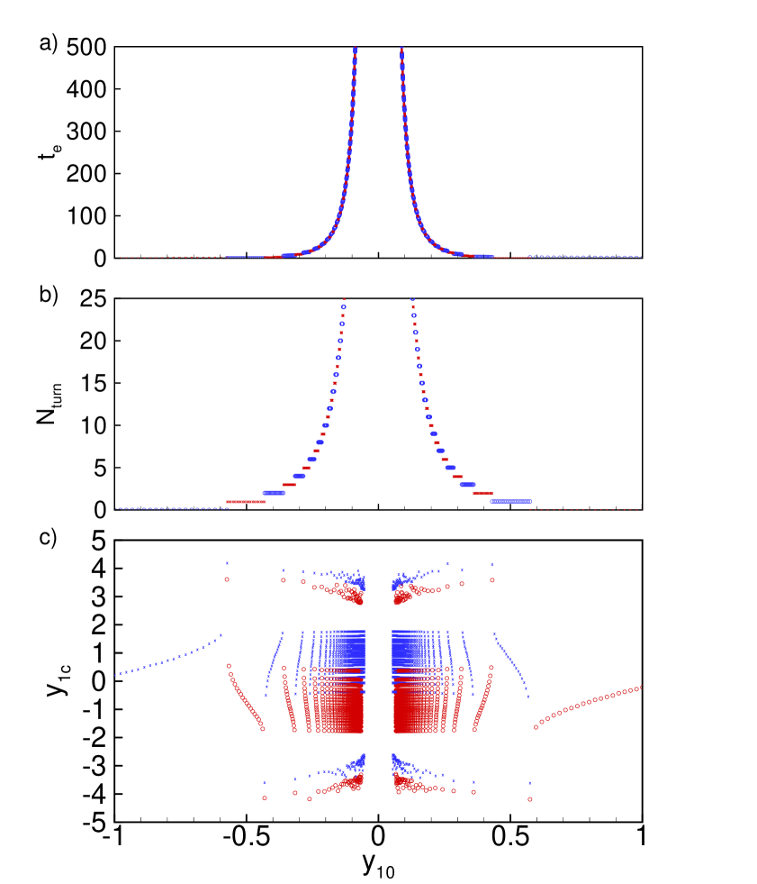
Figure 14: Dependence of the key dynamical variables as a function of the initial condition ${\bf y}_{0}=(y_{10},0)$ on the $y_{1}$=axis for $(n,m)=(3,2.5)$ and $\gamma=10$: exit time $t^{\pm k}({\bf y}_{0})$ on $b^{\pm}$ into the non-oscillatory regime beyond the intervals $\Delta e^{(\pm 1,\mp 0)}$ shown in figure 13 (top panel); $N_{turn}({\bf y}_{0})$ (middle panel); and $y_{1c}({\bf y}_{0})$ (bottom panel). In each panel, “circle” and “crosses” symbols correspond to points in $\triangle e^{+(k+1),-k}$ and $\triangle e^{-k,+(k-1)}$, respectively. Notice the alternate structure in panel c) reflecting the spiralling topology of the boundaries $b^{+}$ and $b^{-}$ shown in figure 13. In order to construct panel c), we have sampled each turn segment $\triangle e^{\pm k+1,\mp k}$ by 20 $y_{10}$ points. The two end points are chosen to be less than 10^-8 away from ${\bf p}^{\pm k+1}$ and ${\bf p}^{\mp k}$. The other 18 points are equally spaced within $\triangle e^{\pm k+1,\mp k}$.

Figure 14 shows these dynamical properties as a function of $y_{10}$ for $(n,m)=(3,2.5)$ with $\gamma=10$ and 1000, determined by direct numerical integration of the equations of motion, using a fifth-order Runge-Kutta integration scheme with adjustable time step. Each discontinuity of $N_{turn}$ and $y_{1c}$ as a function of $y_{10}$ occurs at a turn point ${\bf p}^{\pm k}$ which separates two turn segments, one in $B^{+}$ and the other in $B^{-}$ (Figure 13 and Remark 7.3.10).

$N_{turn}$ is directly associated with the oscillatory behavior of the dynamics. Note that it exhibits a staircase structure, being constant for any point in $\triangle e^{(\pm(k+1),\mp k)}$ (Table 2).

In contrast, $y_{1c}$ is a property more directly associated with the singular behavior and takes identical values for any point ${\bf y}_{0}\in\triangle e^{\pm k,\mp(k-1)}$ which is mapped to $y_{1c}({\bf p}^{(\pm 1,\mp 0)})=\langle\pm\infty,\mp\infty\rangle$ after $k$ turns (Corollary 7.3.14) with $y_{1c}({\bf p}^{\pm k})=\pm\infty$. Moreover, given a $y_{1c}$, each turn segment $\triangle e^{(\pm(k+1),\mp k)}$ has a unique point ${\bf y}_{0}^{(\pm(k+1),\mp k)}$ (Corollary 7.3.14).

The critical or singular time $t_{c}$ is function both of the oscillatory and the singular terms:

$$t_{c}({\bf y}_{0})=t_{c}({\bf p}^{(\pm 1,\mp 0)})-\triangle t_{e}^{(\pm(k+1),\mp k)}~{},$$ (158)

where ${\bf y}_{0}\in\triangle e^{(\pm(k+1),\mp k)}$. However, the explosive singular time scale $t_{c}({\bf p}^{(\pm 1,\mp 0)})$ is generally much shorter than the slow oscillation time scale $\triangle t_{e}^{(\pm(k+1),\mp k)}$ (see figure 9)). Hence, the total time $t_{c}$ needed to reach the singularity is dominated by $\triangle t_{e}^{(\pm(k+1),\mp k)}$.

7.4.2 Definition and mechanism

Our analysis up-to-now has demonstrated a hierarchical organization of the spiraling trajectories diverging away from the origin in phase space, as shown in figure 13. Figure 14 quantifies this hierarchical organization by showing the dependence of the critical time $t_{c}$, the number $N_{\rm turn}$ of rotations of the spiraling trajectory in phase space and the final value $y_{1c}$, as a function of the initial value of $y_{10}\equiv y_{1}(t_{0})$ on the $y_{1}$-axis. The two former quantities diverge as power laws of $y_{10}$ with negative exponents as $y_{10}\to 0$. The last quantity exhibits a “local fractal” structure around the origin which reflects the nested spiral structure of the two basins $B^{+}$ and $B^{-}$ around the origin $S$, and the fact that each turn segment $\triangle e^{(\pm(k+1),\mp k)}$ shares the same singular dynamical properties as $\triangle e^{(\pm 1,\mp 0)}$. Accordingly, $N_{\rm turn}$ is $k+1$ for $y_{10}\in\triangle e^{(\pm(k+1),\mp k)}$

Figure 15 make these statements more quantitative by showing the log-log plots of $t_{c}(y_{10})$, of $\Delta t_{c}(y_{10})$ (defined as the increment of $t_{c}$ over one turn of the spiral starting from a given initial point), of $N_{\rm turn}(y_{10})$ and of the increment $\Delta y_{1}(y_{10})$ over one turn of the spiral, as a function of $(y_{10})$. The observed straight lines qualify power laws. In order to get accurate and reliable estimations of these dependences and of the exponents defined below, we have integrated the dynamical equations using a fifth-order Runge-Kutta integration scheme with adjustable time step.

Figure 16 shows that the exponents (slopes of the log-log plots) are essentially identical for $\gamma=10,100$ and $1000$, indicating that the scaling properties depend only on the exponents $(n,m)$ and are independent of $\gamma$.

These different power laws correspond to the linear behaviors shown in figure 15 and can be represented as follows.

$$N_{\rm turn} \sim y_{10}^{-a}~{},~{}~{}~{}~{}~{}~{}~{}~{}{\rm where}~{}a>0~{},$$ (159)

$$t_{c} \sim y_{10}^{-b}~{},~{}~{}~{}~{}~{}~{}~{}~{}{\rm where}~{}b>0~{},$$ (160)

$$\Delta y_{1} \sim y_{10}^{c}~{},~{}~{}~{}~{}~{}~{}~{}~{}{\rm where}~{}c>0~{},$$ (161)

$$\Delta t_{c} \sim y_{10}^{-d}~{},~{}~{}~{}~{}~{}~{}~{}~{}{\rm where}~{}d>0~{},$$ (162)

where $y_{10}\equiv y_{1}(t_{0})$. Specifically, the definitions are (see figure 16): $\triangle y_{1}=|y_{10}^{+(k+2)}-y_{10}^{+k}|$, $\triangle t_{c}=|t_{c}({\bf p}^{+(k+2)})-t_{c}({\bf p}^{+k})|$, $t_{c}=t_{c}({\bf p}^{+k})$, and $N_{turn}=k$.

The self-similar behavior and power laws occur because there is a countable infinite number of $\Delta e^{\pm(k+1,k)}$ within an extremely slowly-divergent oscillatory source region $S$ which reach the pre-exit basin segment $\Delta e^{(\pm 1,\mp 0)}$ after $k$ mapping (therefore after about $t^{\pm(k+1)}$ exit time interval with $N_{\rm turn}=k+1$ forward turns).

Note that the self-similar behavior close to the origin is governed by the singular boundaries $b^{\pm}$. The choice of the $y_{1}$-axis to define the segments has been made for the simplicity associated with counting number of forward turns. In theory, $y_{1}$-axis can be replaced with any judiciously chosen curve/lines. Here, we choose the $y_{1}$-axis to define the segments, so that the self-similar properties are described as a function of the initial position $y_{10}$ while its velocity $y_{2}$ is set to zero.

7.4.3 Scaling relations from self-consistency

Eliminating $y_{10}$ between (160) and (162) gives

$$\Delta t_{c}\sim t_{c}^{d\over b}~{}.$$ (163)

Since $\Delta t_{c}$ is nothing but the difference $\Delta t_{c}=t_{c}(N_{\rm turn}+1)-t_{c}(N_{\rm turn})$, (163) gives the discrete difference equation on the function $t_{c}(N_{\rm turn})$

$${t_{c}(N_{\rm turn}+\Delta N_{\rm turn})-t_{c}(N_{\rm turn})\over\Delta N_{\rm turn}}\propto t_{c}^{d\over b}~{},$$ (164)

where $\Delta N_{\rm turn}=N_{\rm turn}+1-N_{\rm turn}=1$. The left-hand-side of (164) provides a discrete difference representation of the derivative $dt_{c}/dN_{\rm turn}$. Equation (164) can then be integrated formally to give $N_{\rm turn}\sim t_{c}^{1-{d\over b}}$, which is valid for $d<b$. Comparing with the relation between $N_{\rm turn}$ and $t_{c}$ obtained by eliminating $y_{10}$ between (159) and (160), i.e., $N_{\rm turn}\sim t_{c}^{a\over b}$, we get the scaling relation

$$a=b-d~{}.$$ (165)

Since $a>0$, the condition $d<b$ is automatically satisfied.

Similarly, $\Delta y_{1}=y_{10}(N_{\rm turn}+1)-y_{10}(N_{\rm turn})\propto y_{10}^{c}$ according to definition (161). This gives the differential equation $dy_{10}/dN_{\rm turn}\sim y_{10}^{c}$, whose solution is $N_{\rm turn}\sim 1/y_{10}^{c-1}$, valid for $c>1$. Comparing with the definition (159), we get the second scaling relation

$$a=c-1~{}.$$ (166)

Since $a>0$, the condition $c>1$ is automatically verified.

The scaling relations (166) and (166) are the only two that can be extracted. This shows that the exponents defined in (159-162) are not independent: out of the four exponents $a,b,c,d$, only two of them are independent.

7.4.4 Determination of the critical exponents

To go further, we use the insight provided by sections 5 to 7.3.

Deep in the spiral structure described in the previous section and depicted in figure 13, one full rotation would close on itself in the absence of the trend term and would conserve exactly the Hamiltonian $H$ defined in (41). In this case, we know that one full rotation takes a time equal to the period $T(H)$ given by (62). In the presence of the trend term, one full rotation is not closed but the failure to close is very small especially so very close to the origin. Actually, the failure of the trajectory to close is quantified by the variable $\Delta y_{1}$ introduced in the previous section and used in (161).

The approximation we are going to use is that the value of the period $T(H)$ without the trend term gives the time $\Delta t_{c}$ needed to make one full rotation (notwithstanding the fact that it does not exactly close on itself). This is essentially an adiabatic approximation in which the Hamiltonian $H$ and the period $T(H)$ are assumed to vary sufficiently slowly so that the local period of rotation follows adiabatically the variation of the Hamiltonian $H$.

Equation (62) gives $T(H)\propto H^{1-n\over 2(n+1)}$. From the normalization (48), the amplitude maximum of $y_{1}$ is proportional to $H^{1\over n+1}$. Putting these two relationship together gives

$$\Delta t_{c}\sim|y_{10}|^{1-n\over 2}~{},$$ (167)

which, by comparison with (162) gives

$$d={n-1\over 2}~{}.$$ (168)

We need a second equation to determine completely the other exponents $a,b$ and $c$. It is provided by $dT/dt$, expressed as $dT/dt=(dT/dH)\times(dH/dt)$, where $dT/dH$ is obtained from (64) and $dH/dt$ is given by (128). Estimating $dT/dH$ from (64) is consistent with the above approximation in which a full rotation along the spiral takes the same time as the corresponding closed orbit in absence of the trend term. Expressing $dH/dt$ using (128) involves another approximation, which is similar in spirit to a mean-field approximation corresponding to average out the effect of the trend term over one full rotation. In so doing, we average out the subtle positive and negative interferences between the reversion and trend terms depicted in figure 10. Furthermore, consistent again with the above approximation in which a full rotation along the spiral takes the same time as the corresponding closed orbit in absence of the trend term, we replace $dT/dt$ by $d\Delta t_{c}/dt_{c}$ and obtain

$${d\Delta t_{c}\over dt_{c}}\sim H^{-{3n+1\over 2(n+1)}}~{}|y_{2}|^{m+1}\sim\Delta t_{c}^{3n+1\over n-1}~{}|y_{1}|^{(n+1)(m+1)\over 2}~{},$$ (169)

where the dependence in $\Delta t_{c}$ in the last expression of the right-hand-side is derived by replacing $H$ by its dependence as a function of $T$ (by inverting $T(H)$ given by (62)) and by identifying $T$ and $\Delta t_{c}$. In the last expression, we have replaced the dependence in $y_{2}$ by the dependence in $y_{1}$ by using the normalization (48), leading to $|y_{2}|\sim|y_{1}|^{n+1\over 2}$. Taking the derivative of (163) with respect to $t_{c}$ provides another estimation of ${d\Delta t_{c}\over dt_{c}}$, and replacing $\Delta t_{c}$ in (169) by its dependence as a function of $y_{10}$ as defined by (162) gives finally:

$$a={1\over 2}(n+1)(m+1)-{1\over 2}(3n+1)~{}.$$ (170)

Figure 16 presents a comparison of the theoretical predictions (165), (166), (168), (170) for the exponents $a,b,c,d$ defined by (159)-(162) with an estimation obtained from the direct numerical simulation of the dynamical equations. The lines are the theoretical predictions of the exponents $a,b,c,d$ for $m=2.5$ (solid line), $m=2.75$ (dotted line) and $m=3$ (dashed line) as function of the exponent $n$. The symbols correspond to the exponents obtained by numerical simulation for $\gamma=10$ (square), $\gamma=100$ (diamond) and $\gamma=1000$ (crosses). The agreement is validated to within numerical accuracy. We verify also the independence of the exponents $a,b,c,d$ with respect to the amplitude $\gamma$ of the reversal term.

7.4.5 Time-dependent expression of the envelop of $y_{1}(t;{\bf y}_{0},t_{0})$

We have seen in section 6.2.2 that, after exiting from the spiral in phase space, the dynamics becomes completely controlled by the trend term, while the reversal term responsible for the oscillations becomes negligible. This leads to the asymptotic solution close to $t_{c}$ given by expression (125), which we rewrite here for the sake of comparison:

$$y_{1}(t)\approx y_{1c}-A(t_{c}-t)^{m-2\over m-1}~{},~{}~{}~{}~{}~{}{\rm outside~{}the~{}oscillatory~{}regime}~{},$$ (171)

where $A$ is an amplitude. $y_{1}(t)$ has an infinite slope but a finite value $y_{1c}$ at the critical time $t_{c}$ since $0<(m-2)/(m-1)<1$. The dependence of this finite critical value $y_{1}(t_{c})=y_{1c}$ as a function of $y_{10}$ is shown in figure 14.

In the oscillatory regime, we can also obtain the growth of the amplitude of $y_{1}(t)$ by combining some of the previous scaling laws (159-162). Indeed, taking the ratio of (161) and (162) yields $\Delta y_{1}/\Delta t_{c}\sim y_{10}^{c+d}$. Since $\Delta y_{1}$ corresponds to the growth of the local amplitude $A_{y_{1}}$ of the oscillations of $y_{1}(t)$ due to the trend term over one turn of the spiral in phase space, this turn lasting $\Delta t_{c}$, we identify this scaling law with the equation for the growth rate of the amplitude $A_{y_{1}}$ of $y_{1}$ in this oscillatory regime:

$${dA_{y_{1}}\over dt}\sim A_{y_{1}}^{c+d}~{}.$$ (172)

Its solution is of the form

$$A_{y_{1}}(t)={B\over(t^{*}-t)^{1/b}}~{},~{}~{}~{}~{}~{}{\rm within~{}the~{}oscillatory~{}regime}~{},$$ (173)

where $B$ is another amplitude. We have used the scaling relations (165) and (166) leading to $c+d-1=b$. The time $t^{*}$ is a constant of integration such that $B/(t^{*})^{1\over b}=A_{y_{1}}(t_{0})$, which can be interpreted as an apparent or “ghost” critical time. $t^{*}$ has no reason to be equal to $t_{c}$, in particular since the extrapolation of (173) too close to $t^{*}$ would predict a divergence of $y_{1}(t)$. The dynamical origin of the difference between $t^{*}$ and $t_{c}$ comes from the fact that $t^{*}$ is determined by the oscillatory regime while $t_{c}$ is the sum (158) of two contributions, one from the oscillatory regime and the other from the singular regime.

The prediction (173) is verified accurately from our direct numerical integration of the equations of motion, as shown in figure 17. To get this figure, we rewrite (173) as

$$t=t^{*}-\beta[A_{y_{1}}(t)]^{-b}~{},$$ (174)

where $\beta=B^{-b}$. Note that (174) has the same power law dependence on $y_{1}$ as (160). The reason lies in the fact that, for $y_{10}$ very close to the origin, the duration of the oscillatory regime is overwhelming that of the singular regime. As a consequence, the two power laws (174) and (160) defined in the asymptotic limit $y_{10}\to 0$ should and are the same.

We compare this expression with the numerical simulation using $|y_{1}^{+k}|(t^{+k})$ for $A_{y_{1}}(t)$. The triangles are the data) $(t^{+k},|y_{1}^{+k}|)$ which are fitted to (174) to get $t^{*}$ and $\beta$. The exponent $b$ is fixed to its theoretical value given by (165,168,170). As can be seen from the two panels, $t^{+k}$ as a function of $|y_{1}^{+k}|$ is a straight line as predicted by (174) with a very good precision. The first panel shows the whole calculated range. The second panel shows a magnification close to the exit point of the oscillatory regime. The different straight lines correspond to fits of the data with (174) over different intervals. We obtain respectively

• $t^{*}=0.3857$ and $\beta=0.3381$ for the interval $k\in[1\to 301]$;

• $t^{*}=0.6665$ and $\beta=0.3381$ for the interval $k\in[61\to 301]$;

• $t^{*}=1.9577$ and $\beta=0.3380$ for the interval $k\in[241\to 301]$;

• $t^{*}=2.4330$ and $\beta=0.3380$ for the interval $k\in[271\to 301]$;

• $t^{*}=3.5695$ and $\beta=0.3379$ for the interval $k\in[286\to 301]$.

These five fits performed increasingly deeper within the oscillatory regime exhibit a good stability for the determination of the slope parameter $\beta=0.3380\pm 0.0001$ but an alarmingly strong variation of the “ghost” critical time $t^{*}$. Essentially, we must conclude that it is impossible to determine $t^{*}$ with any reasonable accuracy. There are two reasons for this. First, as the next section 7.4.6 shows, there is a very slow shift or cross-over within the oscillatory regime to the final power law singularity at $t_{c}$. This cross-over corresponds to $y_{1}(t)$ starting off from its initial value with an amplitude growing according to (173) and then crossing over to (171) close to $t_{c}$. Second, while we hoped that the asymptotic behavior (173,174) would become stable deeper within the oscillatory regime, this is counteracted by larger distances of $|y_{1}^{+k}|(t^{+k})$ from the origin, which make the determination of $t^{*}$ more unstable. These difficulties are similar to but stronger than the well-known problems of the accurate determination of critical transition parameters.

Combining (162) with (173) gives the time dependence of the local period $\Delta t_{c}$ of the oscillation in the oscillatory regime:

$$\Delta t_{c}\sim(t^{*}-t)^{d\over b}~{}.$$ (175)

Notice that the local period of the oscillation is not constant but shrinks progressively to zero as time increases. This is qualitatively reminiscent to the log-periodic oscillations discussed in the introduction [49]. Quantitatively, there is a difference which can be characterized as follows. A log-periodic oscillation associated with discrete scale invariance (DSI) corresponds to characteristic time scales $t^{\pm k}$ (for instance, the times of the local maxima of the oscillations) such that

$$t^{\pm(k+1)}-t^{\pm k}\sim 1/\lambda^{k}~{},$$ (176)

where $k>0$ is an integer and $\lambda>1$ is a prefered scaling ratio of DSI. Expression (176) predicts that $t^{*}-t^{\pm k}\sim 1/\lambda^{k}$, i.e., goes to zero exponentially as a function of the index $k$. In contrast, expression (175) can be rewritten

$$t^{\pm(k+1)}-t^{\pm k}\sim(t^{*}-t^{\pm k})^{d\over b}~{}.$$ (177)

Expression (177) predicts that $t^{*}-t^{\pm k}\sim(k^{*}-k)^{1/(1-{d\over b})}$, i.e., the local period goes to zero in a finite number of turns. The log-periodic result is obtained as the limit $d/b\to 1^{-}$, which is reached for $n\to\infty$ and $m\to 2$. We thus have a dynamical theory that provides a mechanism for quasi-log-periodic oscillations with, in addition, a finite number of them due to the cross-over to the non-oscillatory regime. A similar almost log-periodic but nevertheless distinctly different frequency modulation has recently been observed numerically on the average of the logistic map variable close to a tangent bifurcation associated with deterministic intermittency of type I [9]. These “power law periodicity” are originated in the mechanism of reinjection of the iterates on the channel of near-periodic behavior.

7.4.6 Deviation from scaling

Figure 15 and even more so figure 16 have been constructed in the “scaling” regime in which the two approximations used above hold strongly.

1. Adiabatic approximation: the value of the period $T(H)$ calculated without the trend term gives the time $\Delta t_{c}$ needed to make one full rotation (notwithstanding the fact that it does not exactly close on itself). Equivalently, the Hamiltonian $H$ and the period $T(H)$ are assumed to vary sufficiently slowly so that the local period of rotation follows adiabatically the variation of the Hamiltonian $H$.

2. Mean-field approximation: we average out the effect of the trend term over one full rotation. In so doing, we average out the subtle positive and negative interferences between the reversion and trend terms depicted in figure 10. This allowed us to estimate $dH/dt$ using (128).

The theoretical predictions (165), (166), (168), (170) for the exponents $a,b,c,d$ defined by (159)-(162) obtained using these two approximations have been found to be in very good agreement with direct numerical estimations, as shown in figure 16.

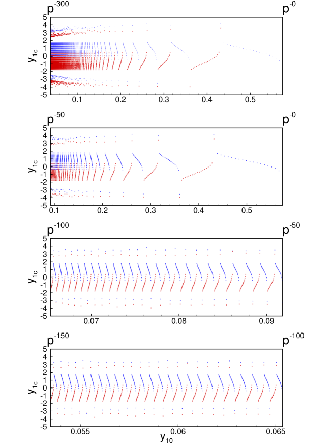
Figure 18: Terminal critical value $y_{1}(t_{c})=y_{1c}$ as a function of initial value $y_{10}$. The top panel shows the oscillations of $y_{1c}$ as a function of $y_{10}$ in the first 300 turn segments $\triangle e^{(\pm(k+1),\mp k)}$ (see definition 7.3.9). Recall that $y_{1c}$ diverges at the boundaries corresponding to the intersection of the two curves $b^{\pm}$ with the $y_{1}$-axis. Due to finite numerical and graphical resolution, we can only observe a cusp-like behavior associated with points approaching very close to these boundaries. The other three panels gives magnifications of the top panel for the first 50 turn segments $\triangle e^{(\pm(k+1),\mp k)}$ (second panel), from the 50th to the 100th turn segments $\triangle e^{(\pm(k+1),\mp k)}$ (third panel) and from the 100th to the 150th turn segments $\triangle e^{(\pm(k+1),\mp k)}$ (fourth panel). In each panel, “circle” and “crosses” symbols correspond to points in $\triangle e^{+(k+1),-k}$ and $\triangle e^{-k,+(k-1)}$, respectively. In order to construct these panels, we have sampled each turn segment $\triangle e^{\pm k+1,\mp k}$ by 20 $y_{10}$ points. The two end points are chosen to be less than $10^{-8}$ away from ${\bf p}^{\pm k+1}$ and ${\bf p}^{\mp k}$. The other 18 points are equally spaced within $\triangle e^{\pm k+1,\mp k}$.

However, this agreement is obtained only within a “scaling” regime, sufficiently close to the origin in phase space, i.e., such that the Hamiltonian $H$ of the oscillations grows sufficiently slowly. To quantify the concept of a “scaling” regime, figure 18 represents the terminal critical value $y_{1}(t_{c})=y_{1c}$ as a function of initial value $y_{1}(t_{0})=y_{10}$ in intervals such that perfect self-similarity can be checked readily. The top panel presents a synopsis by showing the oscillations of $y_{1c}$ as a function of $y_{10}$ for the first 300 turn segments $\triangle e^{(\pm(k+1),\mp k)}$ (see definition 7.3.9). If self-similarity was true, the three following panels in figure 18 should be essentially identical because they show exactly the same number of oscillations. However, it is clear that there is a systematic drift, which is fast at first (second panel for the first 50 turn segments $\triangle e^{(\pm(k+1),\mp k)}$ and then slows down deep within the spiral structure for the third and fourth panel (see figure 13 for definitions).

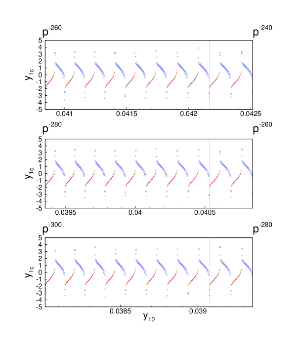
Figure 19: Same as figure 18, i.e., terminal critical value $y_{1}(t_{c})=y_{1c}$ as a function of initial value $y_{10}\equiv y_{1}(t_{0})$ from the 240th to the 260th turn segments $\triangle e^{(\pm(k+1),\mp k)}$ (top panel), from the 260th to the 280th turn segments $\triangle e^{(\pm(k+1),\mp k)}$ (middle panel) and from the 280th to the 300th turn segments $\triangle e^{(\pm(k+1),\mp k)}$ (bottom panel). The two vertical lines provide a guide to the eye to verify the almost perfect self-similarity.

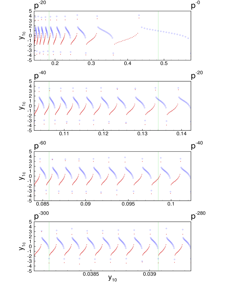
Figure 20: Same as figure 19 from the 0th to the 20th turn segments $\triangle e^{(\pm(k+1),\mp k)}$ (first top panel), from the 20th to the 40th turn segments $\triangle e^{(\pm(k+1),\mp k)}$ (second panel), from the 40th to the 60th turn segments $\triangle e^{(\pm(k+1),\mp k)}$ (third panel) and from the 280th to the 300th turn segments $\triangle e^{(\pm(k+1),\mp k)}$ (fourth bottom panel). The two vertical lines provide a guide to the eye to show that self-similarity is not qualified.

Figure 19 exhibits almost perfect self-similarity by plotting the terminal critical value $y_{1}(t_{c})=y_{1c}$ as a function of initial value $y_{1}(t_{0})=y_{10}$ from the 240th to the 260th turn segments $\triangle e^{(\pm(k+1),\mp k)}$ (top panel), from the 260th to the 280th turn segments $\triangle e^{(\pm(k+1),\mp k)}$ (middle panel) and from the 280th to the 300th turn segments $\triangle e^{(\pm(k+1),\mp k)}$ (bottom panel). The two vertical lines provide a guide to the eye to verify the almost perfect self-similarity. This is the regime and beyond where the scaling laws reported in figures 15 and 16 hold. The cross-over to this scaling regime is presented visually in figure 20 which compares exactly twenty oscillations of the terminal critical value $y_{1}(t_{c})=y_{1c}$ as a function of initial value $y_{1}(t_{0})=y_{10}$ in different intervals, from close to the exit point (first top panel) to deep within the spiral structure (bottom panel). The two vertical lines point out the deviations from the close-to-asymptotic regime of the bottom panel reached from the 280th to the 300th turn segments $\triangle e^{(\pm(k+1),\mp k)}$ as the dynamics gets closer and closer to the exit point (from the third to the first panel).

It is probably possible to improve upon the scaling theory offered in section 7.4.4 and go beyond the adiabatic mean-field approximation in order to describe the cross-over regime between the asymptotic scaling regime and the exit of the spiral structure. This should be done by quantifying the relative reinforcing and opposing effects of the trend and reversal terms within each turn, as shown in figure 10.

8 Concluding remarks

We have introduced a second-order ordinary differential equation describing an oscillator exploding in finite time whose dynamics results from the interplay between a nonlinear negative viscosity and a nonlinear reversal term. This system provides a simplified description of stock market prices, population dynamics and material rupture, in regimes where the growth rates are an increasing function of the price, population or stress, respectively, in the presence of important negative feedback effects. Our approach using dynamical system theory has shown that the trajectories can be understood in details from the spiraling structure of two sets of specials curves in phase space linking the origin to points at infinity.

The message of our work is threefold. First, it is important to take into account the delayed response of dynamical variables to past states, leading technically to the presence of a second (or higher) order differential equation. This inertia is essential for the generation of oscillations resulting from overshooting. Second, positive nonlinear feedback is a general and ubiquitous mechanism for generating accelerated super-exponential growth ending in finite-time singularities. Third, reversal, recovery or healing mechanisms with nonlinear threshold-like behavior, together with inertia, ensure the existence of overshooting and thus of oscillations controlled by the amplitude of the variable. Our two-dimensional nonlinear dynamical system opens the road to a re-examination of many systems which contain these elements but which have been linearized, thus missing the novel phenomenology unraveled here. Our study suggests that super-exponential growth modulated by amplitude-dependent oscillations may be a general feature of complex systems, such as financial markets, population and heterogeneous materials. We believe that this work provides a novel framework to model these systems and to discover new precursory indicators or patterns of “rupture”. This seems to offer a generalization to the reported log-periodic critical oscillations previously reported for these systems (see [49] and references therein).

The study presented here can be enriched in many ways. For several applications, three obvious missing ingredients are additive noise, stochastic reversal to the fixed point $(y_{1}=0,y_{2}=0)$ and saturation effects with reinjection limiting the growth before reaching the singularity. The addition of these terms will naturally lead to intermittent oscillatory structures (deterministic, stochastic, or both resulting from the interplay between deterministic chaos and noise), similar to those documented as log-periodic power laws in financial bubbles [31, 27, 28] as well as in the population dynamics [30] and in rupture [2, 25, 29].

Figure 6: Solution of (119) for the parameters $m=1$, $n=3$, $\alpha=1$, $\gamma=10$, $y_{10}\equiv y_{1}(t=0)=1$ and $y_{20}\equiv dy_{1}/dt|_{t=0}=5$. The amplitude of $y_{1}(t)$ grows exponentially and the accelerating oscillations have their frequency increasing also approximately exponentially with time.

Figure 15: Scaling laws associated with the fractal properties as a function of initial condition at turn points ${\bf y}_{0}=(y_{10}^{+k},0)$ of $b^{+}$ for $y_{1}>0$ on the $y_{1}$-axis for $(n,m)=(3,2.5)$ as in Figure 11: a) $\gamma=10$ and b) $\gamma=1000$. The notations are: $\triangle y_{1}=|y_{10}^{+(k+2)}-y_{10}^{+k}|$, $\triangle t_{e}=t_{e}({\bf p}^{+(k+2)})-t_{e}({\bf p}^{+k})|$, $t_{e}=t^{\pm k}({\bf p}^{+k})$, and $N_{turn}=k$.

Figure 16: Comparison of the theoretical predictions (165), (166), (168), (170) for the exponents $a,b,c,d$ defined by (159)-(162) with estimations obtained from the direct numerical integration of the dynamical equations using a fifth-order Runge-Kutta integration scheme with adjustable time step. The lines are the theoretical predictions as a function of $n$ for $m=2.5$ (solid line), $m=2.75$ (dotted line) and $m=3$ (dashed line) as function of the exponent $n$. The symbols correspond to the exponents obtained by numerical simulation for $\gamma=10$ (square), $\gamma=100$ (diamond) and $\gamma=1000$ (crosses).

Figure 17: Non-parametric test of the prediction (173) by rewriting (173) as (174) so as it qualifies by a linear behavior. The time $t^{+k}$ is plotted (triangles) as a function of $|y_{1}^{+k}|(t^{+k})$ which are proxies for $(A_{y_{1}}(t)$. The triangles are fitted to (174) to get $t^{*}$ and $\beta$. The exponent $b$ is fixed to its theoretical value given by (165,168,170). The first panel shows the whole calculated range. The second panel shows a magnification close to the exit point of the oscillatory regime. The different straight lines corresponds to fits of the data with (174) over different intervals, with $t^{*}=0.3857$ and $\beta=0.3381$ for the interval $k=1\to 301$; $t^{*}=0.6665$ and $\beta=0.3381$ for the interval $k=61\to 301$; $t^{*}=1.9577$ and $\beta=0.3380$ for the interval $k=241\to 301$; $t^{*}=2.4330$ and $\beta=0.3381$ for the interval $k=271\to 301$; $t^{*}=3.5695$ and $\beta=0.3379$ for the interval $k=286\to 301$.

References

- [1] Andersen, J.V., S. Gluzman and D. Sornette (2000) Fundamental Framework for Technical Analysis, European Physical Journal B 14, 579-601.
- [2] Anifrani, J.-C., Le Floc’h, C., Sornette, D. and Souillard, B. (1995) Universal log-periodic correction to renormalization group scaling for rupture stress prediction from acoustic emissions, J. Phys. I France 5, 631–638.
- [3] Bender C, Orszag S.A (1978) page 147 in Advanced Mathematical Methods for Scientists and Engineers (McGraw-Hill, New York).
- [4] Bhattacharjee, A., C.S. Ng and X. Wang (1995) Finite-time vortex singularity and Kolmogorov spectrum in a symmetric three-dimensional model, Phys. Rev. E 52, 5110-5123.
- [5] Bouchaud, J.-P. and R. Cont (1998) A Langevin approach to stock market fluctuations and crashes, Eur. Phys. J. B 6, 543-550.
- [6] Canessa, E. (2000) Multifractality in time series, J. Phys. A 33, 3637-3651.
- [7] Canessa, E. (2000) Economic mapping to the renormalization group scaling of stock markets, preprint cond-mat/0008300
- [8] Carbonara, P. (1999) What is the intrinsic value? Money 28, 133.
- [9] H.L.D. de S. Cavalcante, G.L. Vasconcelos and J.R.R. Leite, Power law periodicity in the tangent bifurcations of the logistic map, Physica A, 291-296 (2001).
- [10] Chiang, R., P. Liu and J. Okunev (1995) Modelling mean reversion of asset prices towards their fundamental value, Journal of Banking & Finance 19, 1327-1340.
- [11] Choptuik M.W (1999) Universality and scaling in gravitational collapse of a massless scalar, Physical Review Letters 70, 9-12; Critical behaviour in gravitational collapse, Progress of Theoretical Physics Supplement 136, 353-365.
- [12] Chowdhury, D. and D. Stauffer (1999) A generalized spin model of financial markets, Eur. Phys. J. B 8, 477-482.
- [13] Cohen J.E. (1995) Population growth and Earth’s human carrying capacity. Science 269: 341-346.
- [14] Cont., R. and Bouchaud, J.-P. (2000) Herd behavior and aggregate fluctuations in financial markets, Macroeconomic Dynamics 4, 170-196.
- [15] Farmer, J.D. (1998) Market force, ecology and evolution, preprint at adap-org/9812005
- [16] Farmer, J.D. and S. Joshi (2001) The price dynamics of common strategies, to appear in the Journal of Economic Behavior and Organization, e-print at
- [17] Garcimartin, A., Guarino, A., Bellon, L. and Ciliberto, S. (1997) Statistical properties of fracture precursors, Phys. Rev. Lett. 79, 3202–3205.
- [18] Gradshtein, I.S. and and I.M. Ryzhik (1994) Table of integrals, series, and products, I.S. Gradshteyn and Alan Jeffrey, editors, translated from the Russian by Scripta Technica, Inc., 5th ed. (Boston: Academic Press), p. 262.
- [19] Grassia, P.S. (2000) Delay, feedback and quenching in financial markets, Eur. Phys. J. B 17, 347-362.
- [20] Guarino, A., Garcimartin, A. and Ciliberto, S. (1998) An experimental test of the critical behaviour of fracture precursors, Eur. Phys. J. B 6, 13-24.
- [21] Guarino, A., Ciliberto, S. and Garcimartin, A. (1999) Failure time and microcrack nucleation, Europhysics Letters 47, 456-461.
- [22] Guckenheimer, J. and Holmes, P. (1997) Nonlinear oscillations, dynamical systems, and bifurcations of vector fields Corr. 5th print. New York :Springer, pp.318-325.
- [23] Hanson R (2000) Could it happen again? Long-term growth as a sequence of exponential modes. Working paper available at .
- [24] Hunt, J.C.R. and Vassilicos, J.C. (1991) Kolmogorov’s contributions to the physical and geometrical understanding of small-scale turbulence and recent developments, Proc. Roy. Soc. Lond. A 434, 183-210.
- [25] Johansen, A. and D. Sornette (1998) Evidence of discrete scale invariance by canonical averaging, Int. J. Mod. Phys. C 9, 433-447.
- [26] Johansen, A. and D. Sornette (1999) Financial “anti-bubbles”: log-periodicity in Gold and Nikkei collapses, Int. J. Mod. Phys. C 10, 563-575.
- [27] Johansen, A. and D. Sornette (1999) Bubbles and anti-bubbles in Latin-American, Asian and Western stock markets: An empirical study, in press in International Journal of Theoretical and Applied Finance (e-print at cond-mat/9907270)
- [28] Johansen A. and Sornette D (2000) The Nasdaq crash of April 2000: Yet another example of log-periodicity in a speculative bubble ending in a crash, Eur. Phys. J. B 17, 319-328.
- [29] Johansen, A. and D. Sornette (2000) Critical ruptures, Eur. Phys. J. B 18, 163-181.
- [30] Johansen, A. and D. Sornette (2001) Finite-time singularity in the dynamics of the world population and economic indices, Physica A 294, 465-502.
- [31] Johansen A, Sornette, D. Ledoit, O. (1999) Predicting Financial Crashes using discrete scale invariance, Journal of Risk 1, 5-32 and references therein.
- [32] Johansen A, Saleur, H., Sornette, D. (2000) New Evidence of Earthquake Precursory Phenomena in the 17 Jan. 1995 Kobe Earthquake, Japan, Eur. Phys. J. B 15, 551-555 and references therein.
- [33] Kapitza, S.P. (1996), Phenomenological theory of world population growth, Uspekhi Fizichskikh Nauk 166, 63-80.
- [34] Kiehn, R.M. (1993) Instability patterns, wakes and topological limit sets, in J.P. Bonnet and M.N. Glauser, eds., “Eddy structure indentification in free turbulent shear flows”, Kluwer Academic Publisher, 363.
- [35] Krajcinovic, D. (1996) Damage mechanics, North-Holland Series in Applied Mathematics and Mechanics, Elsevier, Amsterdam.
- [36] Lamaignère, L., F. Carmona and D. Sornette (1996) Experimental realization of critical thermal fuse rupture, Phys. Rev. Lett. 77, 2738-2741.
- [37] Lamont, O. (1988) Earnings and expected returns, The Journal of Finance LIII, 1563-1587.
- [38] Lee, C.M., J. Myers, B. Swaminathan (1999) What is the intrinsic value of the Dow? Journal of Finance 54, 1693-1741.
- [39] Leoncini, X., L. Kuznetsov, G. M. Zaslavsky (2000) Motion of Three Vortices near Collapse, Phys. Fluids 12, 1911-1927.
- [40] Lux, T. and M. Marchesi (1999) Scaling and criticality in a stochastic multi-agent model of a financial market, Nature 297, 498-500.
- [41] Malkiel B.G., A random walk down Wall Street (1999) W.W. Norton & Company, New York.
- [42] Moffatt H.K (2000) Euler’s disk and its finite-time singularity, Nature 404, 833-834.
- [43] Mulligan, C.B. and Sala-i-Martin, X. (2000) Extensive margins and the demand for money at low interest rates, Journal of Political Economy
- [44] Pandey, R. B., and Stauffer, D. (2000) Search for log-periodicity oscillations in stock market simulations, International Journal of Theoretical and Applied Finance 3, 479-482.
- [45] Pumir A, Siggia E.D (1992) Vortex morphology and Kelvin theorem, Physical Review A 45, R5351-5354.
- [46] Rascle M, Ziti C (1995) Finite-time blow-up in some models of chemotaxis, Journal of Mathematical Biology 33, 388-414.
- [47] Ray, P. and G. Date (1996) Spatial scaling in fracture propagation in dilute systems, Physica A 229, 26-35.
- [48] Sahimi, M. and Arbabi, S. (1996) Scaling laws for fracture of heterogeneous materials and rocks, Phys. Rev. Lett. 77, 3689–3692.
- [49] Sornette D (1998) Discrete scale invariance and complex dimensions, Physics Reports 297, 239-270. updated version available at cond-mat/9707012.
- [50] Sornette, D. (1998) Discrete scale invariance in turbulence? U. Frisch (ed.), Advances in Turbulence VII, (Kluwer Academic Publishers, The Netherlands), pp. 251-254 (e-print at cond-mat/9802121)
- [51] Sornette, D. (2000) Critical Phenomena in Natural Sciences (Chaos, Fractals, Self-organization and Disorder: Concepts and Tools), Springer Series in Synergetics (Springer, Heidelberg).
- [52] Sornette, D. and Vanneste, C. (1992) Dynamics and memory effects in rupture of thermal fuse networks, Phys. Rev. Lett. 68, 612–615.
- [53] Stauffer, D. and D. Sornette (1999) Self-Organized Percolation Model for Stock Market Fluctuations, Physica A 271, 496-506.
- [54] Szydlowski, M., Krawiec, A. and Tobola, J. (2001) Nonlinear oscillations in business cycle model with time lags, Chaos, Solitons and Fractals 12, 505-517.
- [55] Thurner, S. (2000) A dynamical thermostat approach to financial asset price dynamics, preprint cond-mat/0011286
- [56] van Raan A.F.J (2000) On growth, ageing and fractal differentitation of science, Scientometrics 47, 347-362.
- [57] Vanneste, C. and Sornette, D. (1992) Dynamics of rupture in thermal fuse models, J. Phys. I France 2, 1621–1644.
- [58] Vassilicos, J.C. (1995) Anomalous diffusion of isolated flow singularities and of fractal or spiral structures, Phys. Rev. E 52, R5753-R5756.
- [59] Zubarev, N. M. (1998) Formation of root singularities on the dree surface of a conducting fluid in an electric field, Phys. Lett. A 243, 128-131.