[
Lattice Twisting Operators and Vertex Operators in Sine-Gordon Theory in One Dimension
Abstract
In one dimension, the exponential position operators introduced in a theory of polarization are identified with the twisting operators appearing in the Lieb-Schultz-Mattis argument, and their finite-size expectation values measure the overlap between the unique ground state and an excited state. Insulators are characterized by . We identify with ground-state expectation values of vertex operators in the sine-Gordon model. This allows an accurate detection of quantum phase transitions in the universality classes of the Gaussian model. We apply this theory to the half-filled extended Hubbard model and obtain agreement with the level-crossing approach.
pacs:
71.10.Hf,71.10.Pm,75.10.Jm,77.84.-s]
The metal-insulator transition is a fundamental phenomenon in strongly correlated electron systems. An insulator is distinguished from a conductor at zero temperature by its vanishing dc conductivity (Drude weight). Kohn argued that localization of the electric ground-state wave function is the signature of an insulating state[2]. Recently, Resta emphasized that insulators are characterized by their polarizability, and that meaningful definitions are required for the polarization and position operators in extended systems. To this end, he discussed the ground-state expectation value of the exponential of position operators in a finite size system[3, 4, 5],
| (1) |
He showed that the many-body expectation value of position and polarization operators in periodic systems are related to . Generalization and numerical calculations of were also made[4, 6, 7], but our understanding of this quantity is still far from satisfactory. Specifically, we need to know its relation to other theoretical schemes, and to clarify the nature of phase transitions detected by this quantity.
In this Letter, we discuss the quantity from a different point of view. Limiting ourselves to one-dimensional (1D) cases, we give two interpretations to : One is based on the argument by Lieb, Schultz, and Mattis (LSM), which has been applied to spin and electron systems to investigate structure of the excited states[8, 9, 10, 11, 12]. The other is the sine-Gordon theory[13, 14], which describes phase transitions in 1D quantum systems in terms of the renormalization group. We will show that measures the orthogonality between the unique ground state and a specific excited state of the finite size system, and that it also gives the ground-state expectation value of a vertex operator in the bosonization theory. Moreover, we show that the condition corresponds to transition points that belong to the universality class of the Gaussian model, and demonstrate this notion in numerical analysis for a lattice electron model.
First, we discuss the new quantity based on a LSM-type argument using the 1D spinless fermion model (SFM)
| (2) |
where the number of lattice sites is even, is the fermion annihilation operator, and denotes the interaction term given by arbitrary functions of the number operator . The Fermi point is given by where is number of fermions. To make the ground state nondegenerate, we choose periodic (antiperiodic) boundary conditions for odd ( even), based on the Perron-Frobenious theorem. Applying to the ground state with momentum the unitary “twisting operator” times, generates a set of low-lying excited states . is the lattice version of the operator appearing in Eq. (1). The translation operator has eigenvalues . Due to the relation , the operator turns out to move fermions from the left Fermi point () to the right one (). The excitation energy for is evaluated as
| (3) | |||||
| (4) | |||||
Thus, if the state is orthogonal to the ground state , there exists an excited state with energy of .
The orthogonality of these two states depends on the momentum of the excited state . When , where is an integer and is an irreducible fraction, and are characterized by different quantum numbers, so that these two states are orthogonal. On the other hand, when , the two states may not be orthogonal, so that this relation gives a necessary condition for the system to have a gap[11, 12]. The overlap of the two states in a system of size is given by
| (5) |
is real due to parity invariance (). If the system is gapped (gapless), () is expected. However, remains finite in finite-size systems even in gapless cases. The expectation value of the twisting operator is nothing but the quantity underlying Resta’s definitions of electronic localization and polarization[3], and its generalizations[6].
Next, we consider in a different point of view. The low-energy excitations of the SFM (2) with are described by the sine-Gordon model[13, 14]
| (6) | |||||
| (7) |
with a relation . This effective model consists of the Gaussian model and the nonlinear term. Generally, the velocity , the Gaussian coupling , and the Umklapp scattering amplitude are determined phenomenologically. The renormalization group (RG) equations for the nonlinear term are derived under a change of the cutoff [15],
| (8) |
where , , and .
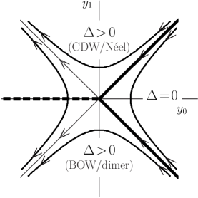
The RG flow of this equation shown in Fig. 1 describes the following three type of transitions: As is well known, the SFM can be mapped on spin chains by a Jordan-Wigner transformation. When the system has SU(2) symmetry, Eq. (7) belongs to universality class of the SU(2)1 symmetric Wess-Zumino-Novikov-Witten (WZNW) model[14], and the parameters are fixed as (). Then, when the initial value of is positive , the nonlinear term is marginally irrelevant [], and the system is gapless. On the other hand, for , the nonlinear term is relevant [], a gap opens, and the phase field is locked in the potential minimum as (mod ). We call the transition at “WZNW type”. In the U(1) symmetric case where the ratio of and is no longer fixed, a Berezinskii-Kosterlitz-Thouless (BKT) -type transition takes place at . For the gapped states , the parameters are renormalized as , and the phase field is locked as (mod ). In the SFM at half-filling (spin chains with zero magnetic field), these two gapped states correspond to the charge-density-wave (Néel) and the bond-order-wave (dimer) states, respectively. On the unstable Gaussian fixed line [ with ], a “Gaussian transition” takes place which is a second-order transition between the two gapped states, and the system is gapless on the transition point. These three transitions can be identified by observing appropriate level crossings in excitation spectra in finite-size systems[16, 17].
Now, let us interpret in terms of the sine-Gordon theory. In the Tomonaga-Luttinger liquid theory which describes the Gaussian fixed point (), the current excitation created by the operator corresponds to the vertex operator [13, 14, 18]. Besides, when , the phase field changes as under a parity transformation, so that given by Eq. (5) is related to the ground-state expectation values of the nonlinear term as
| (9) |
Since the sign of the nonlinear term in Eq. (7) changes at in the RG flow diagram, the WZNW-type and the Gaussian-type transition points can be detected by observing . In the infinite-size limit, we expect () for the gapped (gapless) states.
To demonstrate the above argument, we consider the 1D extended Hubbard model (EHM)
| (10) | |||||
| (11) |
at half-filling and zero magnetic field (). Here is even, and is the electron annihilation operator for spin . The number operators are defined by and . The effective Hamiltonian density of this system is given by sine-Gordon models for the charge () and the spin () sectors and a charge-spin coupling term as[19]
| (12) | |||||
| (13) | |||||
| (14) |
The spin part of this effective model belongs to the universality class of the SU(2)1 WZNW model. According to the level-crossing approach[17], the Gaussian transition in the charge part (), and the WZNW-type spin-gap transition () take place independently near the line with . Therefore, spin-density-wave (SDW), bond-charge-density-wave (BCDW), and charge-density-wave (CDW) phases appear that correspond to the locked phase fields , , and , respectively, where denotes the unlocked (gapless) case.
To apply our argument to this electron system, we introduce the twisting operators for the charge and the spin sectors following Ref. REFERENCES
| (15) |
where . Since this unitary operator corresponds to the vertex operator given by , we obtain the expectation values of the nonlinear terms of Eq. (12) as follows:
| (17) | |||||
| (19) | |||||
Therefore, are expected as , , and for the SDW, BCDW, and CDW regions, respectively, in the limit. We calculate these quantities in finite-size rings (–) numerically. Eigenvalues and eigenstates of the EHM are obtained by the Lanczös algorithm and the inverse iteration method, respectively.
In Fig. 3, we show the numerical results near the line at . For both charge and spin sectors, and change continuously, and change their signs at different points: the Gaussian (BCDW-CDW) and the spin-gap (SDW-BCDW) transitions. Although the convergence of , , and to their saturation values is slow except for the transition points , they are expected to take the predicted values , and change discontinuously at the transition points in the limit.


In Fig. 3, we show the size dependence of the SDW-BCDW and the BCDW-CDW boundaries at determined by the conditions . A benchmark for their accuracy is provided by the level-crossing approach[17] which is also shown. These two methods give quantitatively similar results, so that our interpretation of the by the sine-Gordon theory is confirmed. For extrapolating the critical point to infinite system size, we use given by conformal field theory, which is justified when the non-linear sine-Gordon term is absent. Numerical results equivalent to ours were also obtained in Ref. REFERENCES by observing discontinuities of Berry phases explained in the following. However, the physical interpretations are different. Besides, the present calculation has great advantage in the accuracy and the computational time.
We now discuss the quantity as a complex variable. can be rewritten as a product of the discretized flux state[21, 22]
| (20) |
where with an integer. Here is the ground state for the Hamiltonian with . Now we consider the phase angle of in the complex plane . According to Resta[3], this angle is regarded as the Berry phase [5, 7, 20, 21, 22, 23, 24, 25]
| (21) |
The angle is or according to the signs of , so that it changes discontinuously at the Gaussian- or the WZNW-type transition point [ with ]. However, it also shows a discontinuity on the stable Gaussian fixed line [ with ], which does not correspond to any transitions (see Fig. 1). In this case, becomes meaningless in the limit. For example, this situation appears in the charge sector of the EHM, near the line with [17, 19]. Extending into the complex plane may be useful to distinguish phases with the same . For example, the SFM (2) at half-filling with have a charge-ordered state [] for that gives the same value as that of the bond-order-wave state []. We speculate that their Berry phases are different, e.g. and . It would be interesting to derive a simulation strategy (necessarily involving parity breaking) to support such a conjecture.
In summary, we have given the following two interpretations to Resta’s expectation value of exponential position operators : One is as expectation values of a twisting operator which measures the orthogonality between the unique ground state and an excited state [Eq. (5)]. The other is the ground-state expectation value of the nonlinear term of the sine-Gordon model [Eq. (9)]. From the latter point of view, it is shown that insulating states characterized by correspond to two different fixed points in the RG analysis, and that the condition gives phase transition point which belongs to the Gaussian universality class. We have demonstrated this notion in the EHM, and checked the validity of our argument comparing with the results of the level-crossing approach.
Our work could open significant extensions: The present argument can be applied to spin systems, with e.g. Haldane gaps and magnetization plateaus. The quantity may be applied to higher dimensional cases, since the LSM argument has been extended to these cases by considering a lattice wrapped on a torus[8, 10, 26]. Besides, the quantity can be easily calculated numerically by the density matrix renormalization group method or quantum Monte Carlo simulations, as it is based only on ground-state properties.
One of the authors (M.N.) is grateful to M. Arikawa for discussions. He also learned useful techniques for the exact diagonalization from TITPACK Ver. 2 by H. Nishimori. The research of J.V. was supported by Deutsche Forschungsgemeinschaft through grants no. VO436/6-2 (Heisenberg fellowship) and VO436/7-1.
REFERENCES
- [1]
- [2] W. Kohn, Phys. Rev. 133, A171 (1964).
- [3] R. Resta, Phys. Rev. Lett. 80, 1800 (1998).
- [4] R. Resta and S. Sorella, Phys. Rev. Lett. 82, 370 (1999).
- [5] R. Resta, J. Phys. Condens. Matter 12, R107 (2000).
- [6] A. A. Aligia and G. Ortiz, Phys. Rev. Lett. 82, 2560 (1999).
- [7] A. A. Aligia, K. Hallberg, C. D. Batista, and G. Ortiz, J. Low Temp. Phys. 117, 1747 (1999); Phys. Rev. B 61, 7883 (2000).
- [8] E. Lieb, T. Schultz, and D. Mattis, Ann. Phys. 16, 407 (1961).
- [9] I. Affleck and E. H. Lieb, Lett. Math. Phys. 12, 57 (1986).
- [10] I. Affleck, Phys. Rev. B 37, 5186 (1988).
- [11] M. Oshikawa, M. Yamanaka, and I. Affleck, Phys. Rev. Lett. 78, 1984 (1997).
- [12] M. Yamanaka, M. Oshikawa, and I. Affleck, Phys. Rev. Lett. 79, 1110 (1997).
- [13] J. Voit, Rep. Prog. Phys. 57, 977 (1995).
- [14] A. O. Gogolin, A. A. Nersesyan, and A. M. Tsvelik, Bosonization and Strongly Correlated Systems (Cambridge Univ. Press, 1998).
- [15] J. M. Kosterlitz, J. Phys. C 7, 1046 (1974).
- [16] K. Okamoto and K. Nomura, Phys. Lett. A 169, 433 (1992); K. Nomura and K. Okamoto, J. Phys. A 27, 5773 (1994).
- [17] M. Nakamura, J. Phys. Soc. Jpn. 68, 3123 (1999); Phys. Rev. B 61, 16377 (2000).
- [18] F. D. M. Haldane, J. Phys. C 14, 2585 (1981).
- [19] J. Voit, Phys. Rev. B 45, 4027 (1992).
- [20] M. E. Torio, A. A. Aligia, K. Hallberg, and H. A. Ceccatto, Phys. Rev. B 62, 6991 (2000).
- [21] A. A. Aligia, Europhys. Lett. 45, 411 (1999).
- [22] I. Souza, T. Wilkens, and R. M. Martin, Phys. Rev. B 62, 1666 (2000).
- [23] J. Zak, Phys. Rev. Lett. 62, 2747 (1989); Phys. Rev. B 40, 3159 (1989).
- [24] G. Ortiz and R. M. Martin, Phys. Rev. B 49, 14202 (1994).
- [25] R. Resta and S. Sorella, Phys. Rev. Lett. 74, 4738 (1995).
- [26] M. Oshikawa, Phys. Rev. Lett. 84, 1535 (2000); Phys. Rev. Lett. 84, 3370 (2000).