Pairing in the spin sector

Abstract

The nanometer-scale gap inhomogeneity revealed by recent STM images of BSCCO surface suggests that the “gap coherence length” is of that order. Thus a robust pairing gap can develop despite the poorly screened Coulomb interaction. This can be taken as an evidence that the pairing in high $T_{c}$ materials occurs primarily in the neutral (spin) sector. We provide theoretical support for this point of view.

It was first emphasized to us by Pan and Davis[1] that the energy gap extracted from STM measurements of BSCCO surface is inhomogeneous at nanometer scale. Moreover this is true for systems ranging from under- to slightly over-doping.[2, 3, 4] Pan conjectured that such inhomogeneity is due to the variation of the carrier density in the copper-oxygen plane caused by randomly positioned dopant oxygen.[3]

The above findings suggest that the “gap coherence length” of high-$T_{c}$ materials is at most a few nanometer. Since at such short length scale the Coulomb interaction is poorly screened, it must be true that the pairing takes place primarily in the neutral (spin) sector[5] and hence hardly affects the charge density correlation.

Ever since the BCS theory, superconductivity has been attributed to the pairing of electrons. In the case of high-$T_{c}$ superconductors, it is sometimes stated that superconductivity requires the binding of doped holes. Conceptually it is important to distinguish binding from pairing. The former is a feature in density-density correlation while the latter is manifested in two-particle off-diagonal correlation.

The distinction between pairing and binding is particularly pertinent in the cuprates because of the short gap coherence length. (By gap coherence length we mean the minimum length required for the pairing gap to be exhibited.) Based on the STM results we argue that such length is of order of nanometers. This in turn suggests that the pairing responsible for high-$T_{c}$ superconductivity takes place primarily in the spin degrees of freedom.

We support our point of view by first demonstrating that despite strong Coulomb interaction in the following Hamiltonian

$$H = -t\sum_{\langle ij\rangle}(c_{j\alpha}^{\dagger}c_{i\alpha}\!+h.c.)+J\sum_{\langle ij\rangle}({\bf S}_{i}\cdot{\bf S}_{j}\!-\frac{1}{4}\!n_{i}n_{j})$$ (1)

$$+ {V_{c}}\sum_{i>j}{1\over{r_{ij}}}(n_{i}-\bar{n})(n_{j}-\bar{n}),$$ (2)

it is energetically favorable for the following variational ansatz[5] to develop d-wave pairing:

$$|\Psi(D,\Delta)\rangle=P_{G}|\Psi_{mf}(D,\Delta)\rangle.$$ (3)

Here $P_{G}$ is the projection operator that removes double occupancy and $|\Psi_{mf}(D,\Delta)\rangle$ is the ground state of the following mean-field Hamiltonian

$$H_{mf}(D,\Delta) =\sum_{k}[X_{k}c_{k\sigma}^{\dagger}c_{k\sigma}+iD_{k}c_{k+Q,\sigma}^{\dagger}c_{k\sigma}$$ (5)

$$+(\Delta_{k}c_{k\uparrow}^{\dagger}c_{-k\downarrow}^{\dagger}+{\rm h.c.})],$$

where $X_{k}=-2(\cos k_{x}+\cos k_{y})$, $D_{k}=2D(\cos k_{x}-\cos k_{y})$, and $\Delta_{k}=2\Delta(\cos k_{x}-\cos k_{y})$. In the rest of the paper we use $t/J=3$.

By a straightforward minimization we conclude that for a wide doping range it is energetically favorable to develop a non-zero $\Delta$ (not $D$) for $V_{c}$ as big as $9J$. This result implies that a non-zero $\Delta$ hardly perturb the density-density correlation, hence cannot cause hole binding. We emphasize that the purpose of the present discussion is not to argue that Eq. (3) is the ground state of Eq. (2), rather it is to show that the pairing exhibited by Eq. (3) is not hole binding.

To appreciate the effect of the projection operator in Eq. (3) we have also investigated the stability of $|\Psi_{mf}(0,\Delta)\rangle$ without the Gutzwiller projection. In a nearest-neighbour repulsion model the analytic result suggests that once $V_{nn}$, the nearest-neighbour interaction strength, is larger than $\approx 0.5J$, pairing is absent!

Now we provide the details. We minimize $E(D,\Delta)=\langle\Psi|H|\Psi\rangle/\langle\Psi|\Psi\rangle$ by varying $D$ and $\Delta$. The results presented below are obtained for a system with the average number of holes per site ($x$) equal to $12\%$. The evaluation of $E(D,\Delta)$ is performed by Monte Carlo when necessary.

In Fig.1(a) we present the projected results for $\Delta E\equiv E(0,\Delta)-E(0,0)$ versus $\Delta$ in a $10\times 10$ lattice with 12 holes. The blue open circles are for the pure t-J model, the black crosses are for t-J model with a nearest neighbor repulsion $V_{nn}=3J$, and the red open squares are for t-J + Coulomb model (Eq. (2)) with $V_{c}=3J$. For each of the three cases a nonzero $\Delta$ develops.

In Fig.1(b) we present the corresponding results for the nearest-neighbor repulsion model when the projection operator is removed from the variational ansatz. As one can see even for $V_{nn}=0$ the optimal value of $\Delta$ is suppressed. Moreover for $V_{nn}\geq 0.5J$ the optimal $\Delta$ is zero.

Since the presence/absence of spontaneous staggered current order is a timely issue,[8] we have also studied the optimum form of Eq. (3) allowing both $D$ and $\Delta$. In Fig.1(c) we plot $\Delta E=E(D,\Delta)-E(0,0)$ for the t-J+Coulomb model ($V_{c}=3J$) at $x=12\%$. It is clear from this plot that the minimum corresponds to a non-zero $\Delta$ but $D=0$. Consequently we conclude that for the doping relevant to the present paper d-wave pairing is the only order that occurs for the model described by Eq. (2).

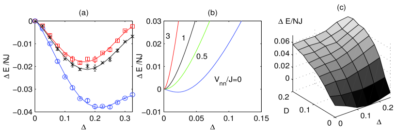
FIG. 1.: Results for $x=12$%. (a) $\Delta E$ as a function of $\Delta$ at $D=0$ from Gutzwiller projection in a $10\times 10$ lattice. Open circles: pure t-J model; crosses: t-J model with nearest neighbor repulsion $V_{nn}=3J$; squares: t-J model with Coulomb interaction $V_{c}=3J$. (b) Without the Gutzwiller projection, analytic results for nearest-neighbor model. c) $\Delta E(D,\Delta)$ as a function of $D$ and $\Delta$ for the projected wavefunction at $V_{c}=3J$.

The next question is, when subjected to disorder potential, whether the wavefunction in Eq. (3) can adjust its pairing parameter $\Delta$ “adiabatically” to the local density to account for the observed gap inhomogeneity. Unfortunately with the disorder potential breaking the translation symmetry the vast variational freedom renders variational Monte-Carlo impossible. What we shall do in the rest of the paper is slave-boson mean-field theory which takes the projection operator in Eq. (3) into account in an average fashion. The hope is that since such mean-field theory qualitatively captures the physics of Eq. (3) in the absence of disorder it will produce meaningful result in its presence.

The starting point of our mean-field theory is the following Hamiltonian[7]

$$H = -t\sum_{\langle ij\rangle}(b_{j}b^{{\dagger}}_{i}f_{j\alpha}^{\dagger}f_{i\alpha}\!+h.c.)+J\sum_{\langle ij\rangle}({\bf S}_{i}\cdot{\bf S}_{j}\!-\frac{1}{4}\!n_{i}n_{j})$$ (6)

$$+ {V_{c}}\sum_{i>j}{1\over{r_{ij}}}(n_{i}-\bar{n})(n_{j}-\bar{n})+\sum_{i}U_{i}n_{i}.$$ (7)

In the above $b$ and $f$ are the holon and spinon operators obeying $f^{\dagger}_{i\alpha}f_{i\alpha}+b^{\dagger}_{i}b_{i}=1$, $n_{i}=1-b^{\dagger}_{i}b_{i}$, and ${\bf S}_{i}=(1/2)f^{\dagger}_{i\alpha}\vec{\sigma}_{\alpha\beta}f_{i\beta}$. The disorder potential $U_{i}$ is given by

$$U_{i}=\sum_{imp=1}^{N_{imp}}{V_{d}\over\sqrt{|{\bf r}_{i}\!-\!{\bf r}_{imp}|^{2}\!+\!d^{2}}}.$$ (8)

In the above ${\bf r}_{imp}$ is the location of the oxygen dopant and $d$, the setback distance, is the vertical separation of the oxygen dopant plane from the copper-oxygen plane.[9] From simple valence counting we expect $N_{imp}$ to be half the number of holes. The results reported in the rest of the paper are obtained on $24\times 24$ lattice for doping $x=12\%$ using $V_{d}/2=V_{c}=t=3J$, and $d=2\times$ the CuO₂ lattice constant. We have checked that the results change smoothly with $d$ and $x$.

The mean-field trial wavefunction $|\psi\rangle$ is given by $|\psi\rangle=|\psi_{b}\rangle\otimes|\psi_{f}\rangle$ where the bosonic $(|\psi_{b}\rangle)$ and fermionic ($|\psi_{f}\rangle)$ states are

$$|\psi_{b}\rangle=[\sum_{j}\chi_{j}b^{\dagger}_{j}]^{N_{b}}|0_{b}\rangle$$ (9)

$$|\psi_{f}\rangle=\prod_{n}[\sum_{j}(u^{*}_{nj}f^{\dagger}_{j\uparrow}+v^{*}_{nj}f_{j\downarrow})]|0_{f}\rangle.$$ (10)

The mean-field single-particle wavefunctions $u_{nj},v_{nj}$ and $\chi_{j}$ are varied to minimize

$$\langle\Psi|H|\Psi\rangle - \sum_{i}\lambda_{i}\langle\Psi|b^{{\dagger}}_{i}b_{i}+f^{{\dagger}}_{i\alpha}f_{i\alpha}-1|\Psi\rangle$$ (11)

$$- \mu\sum_{i}\langle\Psi|n_{i}-\bar{n}|\Psi\rangle.$$ (12)

Lagrange multipliers $\lambda_{i}$, and $\mu$ are introduced to guarantee that the average occupation obeys the constraints locally as well as globally. Assuming that the inhomogeneity in STM images are indeed induced by the dopant disorder, then, this model should capture the essential features of what is seen on BSCCO surface.

The biggest difference between screening in an ordinary metal and in the cuprates is that the latter is close to the Mott-insulating limit. Due to the no-double-occupancy constraint the ability for charge to redistribute is severely hindered. For example while the constraint has no effect on the electron depletion, it does forbid local electron accumulation beyond one electron per site. As a consequence, in the distribution of holes there can be local peaks of hole density while the opposite, i.e. sharp local depletion of holes, tends not to occur. This is indeed what comes out of our calculation.

In Fig. 2 we show the bare impurity potential $U_{i}$ (Fig. 2(a)) and the corresponding hole distribution (Fig. 2(b)). By comparing the two figures, one sees that the hole distribution does correlate with the bare potential.

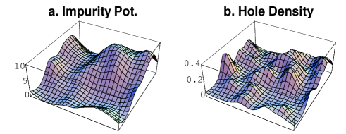
FIG. 2.: A plot of the (a) bare impurity potential $U_{i}$ and (b) the hole distribution (b) in a $24\times 24$ lattice with $x=12\%$ and $d=2$.

We now discuss the mean-field prediction of the tunneling spectroscopy. The local differential conductance measured at a bias $V$ by STM is proportional the electron local density of states. In the slave-boson theory if one writes $b_{i}=|b_{i}|\phi_{i}$ ($\phi$ is a U(1) phase factor) and ignore the fluctuation in $|b_{i}|$, the electron spectral function is given by

$$\rho_{e,i}(V)=|b_{i}|^{2}\rho_{qp,i}(V),$$ (13)

where $\rho_{qp,i}(V)$ is the local spectral function of the quasiparticles and $|b_{i}|^{2}$ is the local hole density. (The quasiparticle creation operator is given by $\phi_{i}f^{\dagger}_{i\alpha}$.) In the mean-field theory where the holon phase fluctuation is ignored one obtains

$$\rho_{qp,i}(V)=\sum_{n}|u_{ni}|^{2}\delta(V\!\!-\!\!E_{n})\!+\!\sum_{n}|v_{ni}|^{2}\delta(V\!\!+\!\!E_{n}).$$ (14)

In the above $(u_{ni},v_{ni})$ is the Bogoliubov-deGennes eigenfunctions of the spinon self-consistent mean-field Hamiltonian.

From Eq. (14) it is clear that when integrated over energy $V$, the quasiparticle spectral function obeys a sum rule,

$$\int_{-\infty}^{\infty}\rho_{qp,i}(V)dV=2,$$ (15)

hence is independent of the site index $i$. This is not true for the electron spectral function. Due to the presence of the $|b_{i}|^{2}$ factor the total integrated value of the electron spectral function depends on the local hole density and hence varies from site to site! Such lack of spectral conservation is a generic property of a Mott insulator[10]. Equation (13) suggests that by properly dividing out the integrated electron density of states (and hence $|b_{i}|^{2}$) one can get the quasiparticle density of states.

It turns out that in the actual experiment this is customarily done. In an STM experiment it is common to have the feedback loop set up so that the total tunneling current (i.e. the integral of the differential conductance up to a voltage V_max) is held at a fixed value[3, 4] This way of calibration precisely divides out $|b_{i}|^{2}$ in Eq. (13). Thus the tunneling spectra presented in Ref.[4] is, in our language, the quasiparticle local density of states. One can also undo the calibration to restore the $|b_{i}|^{2}$ and hence obtain the electron local density of states[3]. It turns out that these two density of states have interesting observable differences.

In Figure 3, we plot the quasiparticle ($\rho_{qp,i}(V)$) and the electron ($\rho_{e,i}(V)$) local density of states in the bias range of $-0.6J\leq V\leq+0.6J$ for four different locations in Fig. 2. Among the four curves the local hole density ($|b_{i}|^{2}$) varies from $0.055$ to $0.174$. As one can see, the peak-to-peak distance, i.e. the local gap, varies considerably among the curves. [3, 4, 2].

Let’s now focus on the behavior of $\rho_{qp,i}(V)$, and $\rho_{e,i}(V)$ at small $V$. While different $\rho_{qp,i}(V)$ curves tend to merge at small voltage, the $\rho_{e,i}(V)$ curves do not. This difference is precisely caused by the fact that each curve has a different $|b_{i}|^{2}$. It is amazing that this difference is seen in the experimental curves by changing the calibration![3, 4]

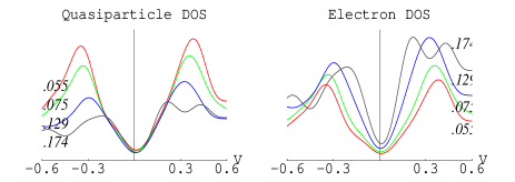
FIG. 3.: Tunneling conductance of the fermions ($\rho_{s,i}(V)$) and of electrons ($\rho_{e,i}(V)$) at several positions in the $24\times 24$ lattice (same as in Fig. 1). The local hole densities corresponding to each curve is indicated in the figure. The bias voltage $V$ is in units of $J$.

What is the reason for the universality of the quasiparticle density of states at low energy? The answer is the robustness of the low-energy quasiparticle wavefunctions due to the vanishing density of states. In Fig. 4 we show $|v_{ni}|^{2}$ for two of the low-lying energy eigenstates (associated with two different nodes) from two different disorder realization, (a)-(b) and (c)-(d) respectively. These eigenstates show a simple, geometric pattern, insensitive to the underlying disorder. The orientation of the wavefunction is also consistent with the direction of the wavevector of the nodal quasiparticles. Such regularity persists up to about $0.15J$, the same energy scale below which the quasiparticle density of states appears universal.

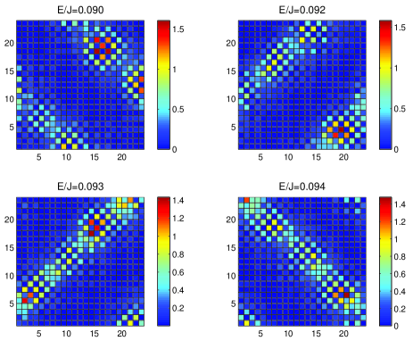
FIG. 4.: Low-lying eigenstates, $|v_{ni}|^{2}$, for two disorder realizations ((a)-(b) and (c)-(d)) for several eigenenergies.

Additional comparison can be made between the experiment and the mean-field result. In Ref. [3], the authors plot the integrated local density of states vs. the local gap. Within the scattering of the data the result follows a monotonic trajectory implying a larger gap for a smaller $|b_{i}|^{2}$ and vice versa. Figure 5 is such a plot from our mean-field theory. (In making this plot we included the local density of states for all 24$\times$ 24 sites in two disordered samples.) The result agrees with the experimental findings qualitatively.

FIG. 5.: Local hole density vs. local peak-to-peak conductance plot.

Before closing a caveat is in order. One aspect of our mean-field result disagrees with the experimental findings – our conductance curves for larger gaps show a taller peak while the experimental finding is the reverse. It is likely that this discrepancy is due to the omission of quantum fluctuation of holon phase ($\phi_{i}$) in our calculation.

It has recently been reported that after thermal annealing, the inhomogeneities of the BSCCO surface disappears. Such result raises question as to whether the observed spectral inhomogeneity is an intrinsic bulk property. The point of view we take in this paper is that even if the surface inhomogeneity is not intrinsic it still tells us an important information, i.e., the existence of a situation where the gap varies on nanometer length scale. We argue that such nanometer-scale variation suggests that the pairing in cuprates occurs essentially in the spin sector.[5, 11]

Acknowledgment  We wish to thank Seamus Davis, Eric Hudson, Kristine Lang, Vidya Madhavan, Joe Orenstein, Shuheng Pan, and Ziqiang Wang for valuable discussions. We are particularly grateful to S.H. Pan and S. Davis’ group for sharing their data with us prior to publication. We are indebted to Ziqiang Wang for suggesting us to look into this problem. DHL is supported in part by NSF grant DMR 99-71503. QHW is supported by the National Natural Science Foundation of China and the Ministry of Science and Technology of China (NKBSF-G19990646), and in part by the Berkeley Scholars Program.

REFERENCES

- [1] Shuheng Pan and Seamus Davis, private communication.
- [2] C. Howald, P. Fournier, and A. Kapitulnik, cond-mat/0101251.
- [3] S. H. Pan et al. Submitted to Nature.
- [4] V. Madhavan et al, Bull. Amer. Phys. Soc. 45 416 (2000); K. Lang et al, Bull. Amer. Phys. Soc. 46, 804 (2001); K. Lang, Ph. D. Thesis, UC Berkeley, 2001.
- [5] P. W. Anderson, Science, 235, 1196 (1987).
- [6] M. G. Zacher et al. Phys. Rev. Lett. 85, 2585 (2000).
- [7] G. Kotliar and J. Liu, Phys. Rev. B 38, 5142 (1988).
- [8] C. Nayak, Phys. Rev. B 62, 4880 (2000); D. A. Ivanov, P. A. Lee, and Xiao-Gang Wen, Phys. Rev. Lett. 84, 3958 (2000); S. Chakravarty, R. B. Laughlin, D. K. Morr and C. Nayak, Phys. Rev. B 63, 094503 (2001); J. H. Han, Qiang-Hua Wang, and D.-H. Lee, Phys. Rev. B (in press); J. B. Marston and A. Sudbo, cond-mat/0103120.
- [9] In the real material, each copper-oxygen plane is influenced by all the dopant layers, not just one, through long-range interaction. Therefore in this paper should be regarded as an effective distance.
- [10] Jung Hoon Han and D.-H. Lee, Phys. Rev. Lett. 85, 1100 (2000).
- [11] V. J. Emery, S. A. Kivelson, and O. Zachar, Phys. Rev. B 59, 15641 (1999).