Magnetization reversal by uniform rotation
(Stoner–Wohlfarth model) in f.c.c. cobalt nanoparticles

Abstract

The combination of high sensitive superconducting quantum interference device (SQUID) with high quality nanoparticles allowed to check the simplest classical model describing the magnetisation reversal by uniform rotation which were proposed more than 50 years ago by Néel, Stoner and Wohlfarth. The micrometer sized SQUIDs were elaborated by electron beam lithography and the nanoparticles were synthesised by arc-discharge. The measured angular dependence of switching fields of nearly all f.c.c. Co nanoparticles revealed a dominating uniaxial magnetic anisotropy. This result suggests that twin boundaries and stacking faults strongly alter the cubic magnetocrystalline anisotropy leading to dominating uniaxial anisotropy. However, few particles were sufficiently ”perfect” in order to show a more complex switching field surface and a field path dependence of the switching field which is the important signature of the cubic magnetocrystalline anisotropy.

For a sufficiently small magnetic sample it is energetically unfavourable to form a stable magnetic domain wall. The specimen then behaves as a single magnetic domain [1]. For the smallest single-domain particles, the magnetisation is expected to reverse by uniform rotation of magnetisation. For somewhat larger ones, nonuniform reversal modes are more likely–for example, the curling reversal mode. In this paper, we discuss in detail the uniform rotation mode that is used in many theories, in particular in Néel, Brown, and Coffey’s theory of magnetisation reversal by thermal activation [2] and in the theory of macroscopic quantum tunnelling of magnetisation [3]. For a review, see Ref. [4].

I Generalisation of the Stoner–Wohlfarth model

The model of uniform rotation of magnetisation, developed by Stoner and Wohlfarth [5] and Néel [6], is the simplest classical model describing magnetisation reversal. One considers a particle of an ideal magnetic material where exchange energy holds all spins tightly parallel to each other, and the magnetisation magnitude does not depend on space. In this case the exchange energy is constant, and it plays no role in the energy minimisation. Consequently, there is competition only between the anisotropy energy of the particle and the effect of the applied field.

The original model of Stoner and Wohlfarth assumed only uniaxial shape anisotropy with one anisotropy constant—that is, one second-order term. This is sufficient to describe highly symmetric cases like a prolate spheroid of revolution or an infinite cylinder. However, real systems are often quite complex, and the anisotropy is a sum of mainly shape (magnetostatic), magnetocrystalline, magnetoelastic, and surface anisotropy. One additional complication arises because the different contributions of anisotropies are often aligned in an arbitrary way one with respect to each other. All these facts motivated a generalisation of the Stoner–Wohlfarth model for an arbitrary effective anisotropy which was done by Thiaville [7, 8].

Similar to the Stoner–Wohlfarth model, one supposes that the exchange interaction in the particle couples all the spins strongly together to form a giant spin whose direction is described by the unit vector $\vec{m}$. The only degrees of freedom of the particle’s magnetisation are the two angles of orientation of $\vec{m}$. The reversal of the magnetisation is described by the potential energy

$$E(\vec{m},\vec{H})=E_{0}(\vec{m})-\mu_{0}VM_{\rm s}\vec{m}.\vec{H}$$ (1)

where $V$ and $M_{s}$ are the magnetic volume and the saturation magnetisation of the particle respectively, $\vec{H}$ is the external magnetic field, and $E_{0}(\vec{m})$ the magnetic anisotropy energy which is given by

$$E_{0}(\vec{m})=E_{\rm shape}(\vec{m})+E_{\rm MC}(\vec{m})+E_{\rm surface}(\vec{m})+E_{\rm ME}(\vec{m})$$ (2)

$E_{\rm shape}$ is the magnetostatic energy related to the particle shape. $E_{\rm MC}$ is the magnetocrystalline anisotropy (MC) arising from the coupling of the magnetisation with the crystalline lattice, similar as in bulk. $E_{\rm surface}$ is due to the symmetry breaking and surface strains. In addition, if the particle experiences an external stress, the volumic relaxation inside the particle induces a magnetoelastic (ME) anisotropy energy $E_{\rm ME}$. All these anisotropy energies can be developed in a power series of $m_{x}^{a}m_{y}^{b}m_{z}^{c}$ with $p=a+b+c=2,4,6,\ldots$ giving the order of the anisotropy term. Shape anisotropy can be written as a biaxial anisotropy with two second-order terms. Magnetocrystalline anisotropy is in most cases either uniaxial (hexagonal systems) or cubic, yielding mainly second- and fourth-order terms. Finally, in the simplest case, surface and magnetoelastic anisotropies are of second order.

Thiaville proposed a geometrical method to calculate the particle’s energy and to determine the switching field for all angles of the applied magnetic field yielding the critical surface of switching fields which is analogous to the Stoner–Wohlfarth astroid.

The main interest of Thiaville’s calculation is that measuring the critical surface of the switching field allows one to find the effective anisotropy of the nanoparticle. The knowledge of the latter is important for temperature-dependent studies and quantum tunnelling investigations. Knowing precisely the particle’s shape and the crystallographic axis allows one to determine the different contributions to the effective anisotropy.

II Uniform Rotation with cubic anisotropy

We have seen in the previous studies [9, 10, 11, 12] that the magnetic anisotropy is often dominated by second-order anisotropy terms. However, for nearly symmetric shapes, fourth-order terms can be comparable or even dominant with respect to the second-order terms. Therefore, it is interesting to discuss further the features of fourth order terms. We restrict the discussion to the 2D problem [7, 13] (see Ref. [8] for 3D).

The reversal of the magnetisation is described by Eq. (1) that can be rewritten in 2D

$$E(\theta)=E_{0}(\theta)-\mu_{0}vM_{\rm s}(H_{x}\cos(\theta)+H_{y}\sin(\theta))$$ (3)

where $v$ and $M_{s}$ are the magnetic volume and the saturation magnetisation of the particle, respectively, $\theta$ is the angle between the magnetisation direction and $x$, $H_{x}$ and $H_{y}$ are the components of the external magnetic field along $x$ and $y$, and $E_{0}(\theta)$ is the magnetic anisotropy energy. The conditions of critical fields ($\partial E/\partial\theta=0$ and $\partial E^{2}/\partial\theta^{2}=0$) yield a parametric form of the locus of switching fields

$$H_{x}=-\frac{1}{2\mu_{0}vM_{\rm s}}\left(\sin(\theta)\frac{dE}{d\theta}+\cos(\theta)\frac{d^{2}E}{d\theta^{2}}\right)$$ (4)

$$H_{y}=+\frac{1}{2\mu_{0}vM_{\rm s}}\left(\cos(\theta)\frac{dE}{d\theta}-\sin(\theta)\frac{d^{2}E}{d\theta^{2}}\right)$$ (5)

As an example we study a system with uniaxial shape anisotropy and cubic anisotropy. The total magnetic anisotropy energy can be described by

$$E_{0}(\theta)=vK_{1}\sin^{2}(\theta+\theta_{0})+vK_{2}\sin^{2}(\theta)\cos^{2}(\theta)$$ (6)

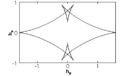
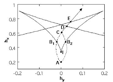
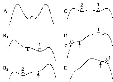
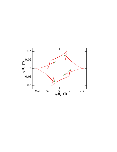
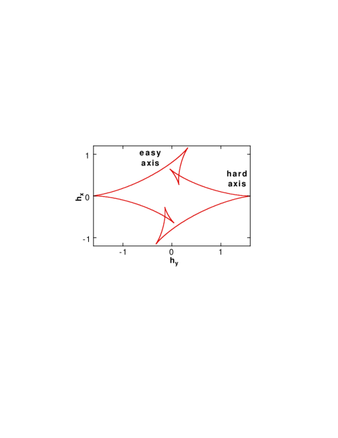
where $K_{1}$ and $K_{2}$ are anisotropy constants ($K_{1}$ could be a shape anisotropy and $K_{2}$ the cubic crystalline anisotropy of a f.c.c. crystal.) $\theta_{0}$ is a constant which allows to turn one anisotropy contribution with respect to the other one. Fig. 1 displays an example of a critical curve which can easily be calculated from Eqs. (4)–(6). When comparing the standard Stoner–Wohlfarth astroid with Fig. 1, we can realise that the critical curve can cross itself several times. In this case, the switching field of magnetisation depends on the path followed by the applied field. In order to understand this point, let us follow the energy potential [Eqs. (3) and (6)] when sweeping the applied field as indicated in Fig. 2. When the field is in A, the energy $E$ has two minima and the magnetisation is in the metastable potential well. As the field increases, the metastable well becomes less and less stable. Let us compare two paths, one going along A $\rightarrow$ B₁ $\rightarrow$ C $\rightarrow$ D $\rightarrow$ E, the other over B₂ instead of B₁. Fig. 3 shows $E$ in the vicinity of the metastable well for different field values along the considered paths (the stable potential well is not presented). One can realise that the state of the magnetisation in C depends on the path followed by the field: Going over B₁ leads to the magnetisation state in the left metastable well (1), whereas going over B₂ leads to the right metastable well (2). The latter path leads to magnetisation switching in D, and the former one leads to a switching in E. Note that a small magnetisation switch happens when reaching B₁ or B₂. Point I is a supercritical bifurcation.

FIG. 1.: Angular dependence of the switching field obtained from Eqs. (4)–(6) with $K_{1}>0$ and $K_{2}=-2/3K_{1}$. The field is normalised by the factor $2K_{1}/(\mu_{0}M_{\rm s})$.

FIG. 2.: Enlargement of angular dependence of the switching field of Fig. 1. Two possible paths of the applied field are indicated: Starting from point A and going over the point B₁ leads to magnetisation reversal in E, whereas going over the point B₂ leads to reversal in D.

FIG. 3.: Scheme of the potential energy near the metastable state for different applied fields as indicated in Fig. 2. The balls represent the state of the magnetisation, and the arrows locate the appearing or disappearing well.

III Experimental evidence for magnetisation reversal by uniform rotation

In order to demonstrate experimentally the uniform rotation mode, the angular dependence of the magnetisation reversal has often been studied (see references in Ref. [1]). However, a comparison of theory with experiment is difficult because magnetic particles often have a nonuniform magnetisation state that is due to rather complicated shapes and surfaces, crystalline defects, and surface anisotropy. In general, for many particle shapes the demagnetisation fields inside the particles are nonuniform leading to nonuniform magnetisation states [1].

An example are ultrathin magnetic dots with in-plane uniaxial anisotropy showing switching fields that are very close to the Stoner–Wohlfarth model, although magnetic relaxation experiments clearly showed that nucleation volumes are by far smaller than an individual dot volume [14] being in agreement with calculations [15]. These studies show clearly that switching field measurements as a function of the angles of the applied field cannot be taken unambiguously as a proof of a Stoner–Wohlfarth reversal.

The first clear demonstration of the uniform reversal mode has been found with Co nanoparticles [9], and BaFeO nanoparticles [10], the latter having a dominant uniaxial magnetocrystalline anisotropy. The three-dimensional angular dependence of the switching field measured on BaFeO particles of about 20 nm could be explained with the Stoner–Wohlfarth model taking into account the shape anisotropy and hexagonal crystalline anisotropy of BaFeO [11]. This explication were supported by temperature- and time-dependent measurements yielding activation volumes which are very close to the particle volume. More recently, the three-dimensional switching field measurements of individual 3 nm Co nanoparticles showed also the uniform reversal mode with dominant uniaxial magnetocrystalline anisotropy which was dominated by surface anisotropy (particle–matrix interface) [12].

The study of uniform rotation for particles with dominating cubic anisotropy revealed to be very difficult because nearly all structural defects in particles lead to dominating uniaxial anisotropy. Nevertheless, we could find few particles which were sufficiently ”perfect” in order to show clearly a field path dependence of the switching field (Fig. 1) which is the important signature of strong higher order terms in the potential energy (Eq. (1). The first measurement of such a field path dependence of switching fields were performed on single-domain FeCu nanoparticles of about 15 nm with a cubic crystalline anisotropy and a small arbitrarily oriented shape anisotropy [16]. Here we report on the magnetic study of individual single-domain cobalt nanoparticles encapsulated in a carbon envelope which provides a very efficient protection against oxidation. Our results show an experimental agreement with the simple classical model mentioned above.

FIG. 4.: TEM image of an assembly of typical cobalt nanoparticles encapsulated in a few graphitic sheets and a large amount of amorphous carbon. Most of the particles have a spherical shape checked through tilting experiments and frequently contain planar defects (see arrows).

FIG. 5.: (a) HRTEM image of a typical single-crystalline f.c.c.–Co nanoparticle in $<$110$>$ projection. Only 3 or 4 graphite sheets imaged by $<$002$>$ lattice fringes with a separation of 0.34 nm are stacked parallel to its surface. Amorphous carbon surrounds the graphite envelope. (b) enlargement of (a) (digitised and Fourier filtered image) showing the ’ABC’ type stacking of $<$111$>$ dense atomic layers which is characteristic of the f.c.c. structure. The slight deviation we noted in angles measurements is attributed to distortions of the structure induced by the interface between the nanocrystal and its graphitic envelope.

A Synthesis of nanoparticles

The arc-discharge method using two graphite electrodes has initially been developed for the synthesis of fullerenes [17, 18] and carbon nanotubes [19] and has been then adapted to the production of endohedral fullerenes and carbon coated nanocrystallites. This technique was used to synthesise the cobalt nanoparticles encapsulated in carbon: the graphite anode was drilled and packed with a mixture of graphite and pure cobalt powders [20]. A plasma was established in the helium atmosphere under the following conditions : 0.6 bar, 25-30 V, 100-105 A dc, during 45 minutes. The deposit formed on the graphite cathode was ground, ultrasonically dispersed in ethanol and put on a holey carbon film for Transmission Electron Microscopy (TEM).

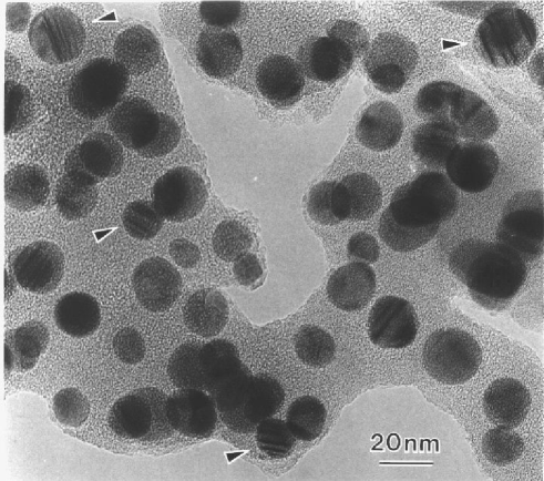
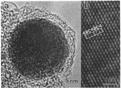
The cobalt nanoparticles are very abundant whereas only a few partially filled carbon nanotubes can be found. Most of the nanocrystals have a spherical shape with a diameter ranging from 5 to 30 nm (Fig. 4). All the particles are coated by carbon. For particles smaller than 10 nm in diameter, the carbon coating is amorphous whereas large particles are encapsulated in graphitic cages and their shape is more polyhedral. Most of the particles have only 3 or 4 graphitic sheets stacked parallel to their surface and are surrounded with amorphous carbon. No void has been observed between the crystallite and the carbon envelope which avoids the oxidation on the surface of the particles that could dramatically affect the magnetic properties.

The crystallites are pure cobalt and have a face-centered cubic (f.c.c.) structure according to the electron diffraction patterns obtained from assemblies of particles. However, the presence of a small amount of hexagonal close-packed (h.c.p.) particles cannot be excluded. Fig. 5 shows an High Resolution TEM image of a typical f.c.c.-Co nanoparticle in a $<$110$>$ projection and encapsulated in 3 or 4 graphitic sheets. No evidence of cobalt carbides has been found. This indicates that the particles were formed at high temperature and rapidly quenched since f.c.c.-Co is the high temperature phase and h.c.p.-Co and cobalt carbides are not stable above 500^∘C. The nanoparticles are mostly single-crystals and often contain twin boundaries and stacking faults (Fig. 4) since these planar defects are known to occur frequently in f.c.c.-Co. As revealed by the HRTEM images, the surface roughness generally does not exceed 2 or 3 atomic layers : this is another important point for the quality of particles with regard to the magnetic properties.

FIG. 6.: Top view and side view of the experimental three-dimensional angular dependence of the switching field of a 20 nm Co particle at 35 mK. This surface is inversion symmetrical with respect to the origin ($H$ = 0). Continuous lines on the surface are contour lines on which $\mu_{0}H_{z}$ is constant.

B Measurement technique

We studied the magnetic properties of individual nanoparticles by using planar Nb micro-bridge-DC-SQUIDs (of about 1 $\mu$m) [9]. In order to place one nanoparticle on the SQUID detector, we disperse the particles in ethanol by ultrasonication. Then we place a drop of this liquid on a chip of about one hundred SQUIDs. When the drop is dry the nanoparticles stick on the chip due to Van der Waals forces. Only in the case when a nanoparticle falls on a micro-bridge of the SQUID loop, the flux coupling between SQUID loop and nanoparticle is strong enough for our measurements. Finally we determine the exact position and shape of the nanoparticles by scanning electron microscopy.

The switching fields of the magnetisation of single Co nanoparticles were measured by using the cold mode method and the blind mode method described in detail in Ref. [21, 22].

FIG. 7.: Top view and side view of the experimental three-dimensional angular dependence of the switching field of a 15 nm Co particle at 35 mK. This surface is inversion symmetrical with respect to the origin ($H$ = 0). Continuous lines on the surface are contour lines on which $\mu_{0}H_{z}$ is constant.

C Results

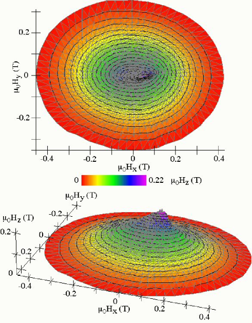
The measured angular dependence of switching fields of nearly all Co nanoparticles revealed a dominating uniaxial magnetic anisotropy similar to previous measurements [9]. Fig. 6 presents a typical example. We estimated the shape anisotropy of the typical nearly spherical nanoparticles (Fig. 4) and found that the shape anisotropy constants should be of the order of magnitude of $10^{4}$ J/m³, i.e. one order of magnitude smaller than the value of the bulk f.c.c. cobalt [23]. This result suggests that twin boundaries and stacking faults (Fig. 4) strongly alter the cubic crystal symmetry leading to dominating uniaxial anisotropy.

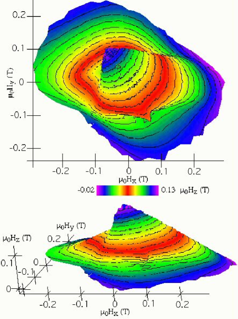
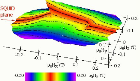
Nevertheless, we could find few particles which were sufficiently ”perfect” in order to show a more complex switching field surface and a field path dependence of the switching field (Fig. 1) which is the important signature of strong higher order terms in the potential energy (Eq. 1). One example is presented in Figs. 7–9. Note that this surface has two easy axes. In addition, the hard plan is deformed. Such a surface can, in principle, be generated by the generalised Stoner-Wohlfarth model when taking into account that the different contributions of anisotropies are aligned in an arbitrary way one with respect to each other.

In order to understand this point qualitatively, let’s come back to the simple 2D case (Eq. 6) where $\theta_{0}$ is a constant which allows to turn the uniaxial shape anisotropy with respect to the cubic anisotropy. Fig. 10 shows the angular dependence of the switching field for a misalignment of $\theta_{0}=10^{\circ}$ which leads to a strong deformation of the curve in Fig. 1.

FIG. 8.: Same data as in Fig. 7. Continuous lines on the surface are contour lines which are parallel to the SQUID plane (defined by $H_{z}$ = 0).

FIG. 9.: Cut of the angular dependence of the switching field as indicated in Fig. 8 (SQUID plane). A clear field path dependence of the switching field was found (Figs. 1 – 2) which shows a strong influence of the cubic crystalline anisotropy.

FIG. 10.: Angular dependence of the switching field obtained from Eqs. (4)–(6) with the same constants as in Fig. 1 but with $\theta_{0}=10^{\circ}$.

IV Conclusion

We used the micro-SQUID technique to study high quality nanoparticles which were synthesised by arc-discharge. The angular dependence of switching fields could be understood in the frame of the simplest classical model describing the magnetisation reversal by uniform rotation. This model were proposed more than 50 years ago by Néel, Stoner and Wohlfarth. The measured critical surface can be considered as a geometrical representation of the magnetic anisotropy of the nanoparticle. Nearly all f.c.c. Co nanoparticles revealed a dominating uniaxial magnetic anisotropy. This result suggests that twin boundaries and stacking faults strongly alter the cubic magnetocrystalline anisotropy leading to dominating uniaxial anisotropy. However, few particles were sufficiently ”perfect” in order to show a more complex switching field surface and a field path dependence of the switching field. The latter is the important signature of the cubic magnetocrystalline anisotropy.

REFERENCES

- [1] Aharoni, An Introduction to the Theory of Ferromagnetism (Oxford University Press, London, 1996).
- [2] W. T. Coffey, D. S. F. Crothers, J. L. Dormann, Yu. P. Kalmykov, E. C. Kennedy, and W. Wernsdorfer, Phys. Rev. Lett. 80, 5655 (1998).
- [3] Quantum Tunneling of Magnetization-QTM’94, Vol. 301 of NATO ASI Series E: Applied Sciences, edited by L. Gunther and B. Barbara (Kluwer Academic Publishers, London, 1995).
- [4] W. Wernsdorfer, Adv. Chem. Phys. 118, 99 (2001).
- [5] E. C. Stoner and E. P. Wohlfarth, Philos. Trans. London Ser. A 240, 599 (1948), reprinted in IEEE Trans. Magn. MAG-27, 3475 (1991).
- [6] L. Néel, C. R. Acad. Science 224, 1550 (1947).
- [7] A. Thiaville, J. Magn. Magn. Mat. 182, 5 (1998).
- [8] A. Thiaville, Phys. Rev. B 61, 12221 (2000).
- [9] W. Wernsdorfer, E. Bonet Orozco, K. Hasselbach, A. Benoit B. Barbara, N. Demoncy, A. Loiseau, D. Boivin, H. Pascard, and D. Mailly, Phys. Rev. Lett. 78, 1791 (1997).
- [10] W. Wernsdorfer, E. Bonet Orozco, K. Hasselbach, A. Benoit, D. Mailly, O. Kubo, H. Nakano, and B. Barbara, Phys. Rev. Lett. 79, 4014 (1997).
- [11] E. Bonet, W. Wernsdorfer, B. Barbara, A. Benoit, D. Mailly, and A. Thiaville, Phys. Rev. Lett. 83, 4188 (1999).
- [12] M. Jamet, W. Wernsdorfer, C. Thirion, D. Mailly, V. Dupuis, P. Mélinon, and A.Pérez, Phys. Rev. Lett. 86, 4676 (2001).
- [13] Ching-Ray Chang, J. Appl. Phys. 69, 2431 (1991).
- [14] O. Fruchart, J.-P. Nozieres, W. Wernsdorfer, and D. Givord, Phys. Rev. Lett. 82, 1305 (1999).
- [15] O. Fruchart, B. Kevorkian, and J. C. Toussaint, Phys. Rev. B 63, 174418 (2001).
- [16] E. Bonet, W. Wernsdorfer, B. Barbara, K. Hasselbach, A. Benoit, and D. Mailly, IEEE Trans. Mag. 34, 979 (1998).
- [17] H.W. Kroto, J.R. Heath, S.C. O’Brien, R.F. Curl, and R.E. Smalley, Nature 318, 162 (1985).
- [18] W. Kratschmer, L.D. Lamb, K. Fostiropoulos, and D.R. Huffman, Nature 347, 354 (1990).
- [19] S. Iijima, J. Appl. Phys. 354, 57 (1991).
- [20] C. Guerret-Piécourt, Y. Le Bouar, A. Loiseau, and H. Pascard, Nature 372, 761 (1994).
- [21] W. Wernsdorfer, D. Mailly, and A. Benoit, J. Appl. Phys. 87, 5094 (2000).
- [22] C. Thirion, W. Wernsdorfer, M. Jamet, D. Mailly, V. Dupuis, P. Mélinon, and A.Pérez, J. Magn. Magn. Mat. 1, 1 (2001).
- [23] C. H. Lee et al., Phys. Rev. B 42, 1066 (1990).