Percolation, Renormalization and the Quantum-Hall Transition

Abstract

In this article, I give a pedagogical introduction and overview of percolation theory. Special emphasis will be put on the review of some of the most prominent of the algorithms that have been devised to study percolation numerically. At the central stage shall be the real-space renormalization group treatment of the percolation problem. As a rather novel application of this approach to percolation, I will review recent results using similar real-space renormalization ideas that have been applied to the quantum Hall transition.

1 Introduction

Imagine a large chessboard, such as occasionally found in a park. It is fall, and all the master players have fled the cold a long time ago. You are taking a walk and enjoy the beautiful sunny afternoon, all the colors of the Indian summer in the trees and in the falling leaves around you. Looking at the chessboard, you see that some squares are already full of leaves, while others are still empty fall . The pattern of the squares which are covered by leaves seems rather random. As you try to cross the chessboard, you see that there is a way to get from one side of the board to the opposite side by walking on leaf-covered squares only. This is percolation — nearly.

Before continuing and explaining in detail what percolation is about, let me outline the content of this paper. In Sect. 2, I will review some of the most prominent and interesting results on classical percolation. Percolation theory is at the heart of many phenomena in statistical physics that are also topics in this book. Beyond the exact solutions of percolation in $d=1$ and $d=\infty$ dimensions, further exact solutions in $2\leq d<\infty$ only rarely exist. Thus computational methods, using high-performance computers and algorithms are needed for further progress and in Sects. 2.2 – 2.4, I explain in detail some of these algorithms. Section 3 is devoted to the real-space renormalization group (RG) approach to percolation. This provides an independent and very suggestive method of analytically computing results for the percolation problem as well as a further numerical algorithm.

While many applications of percolation theory are mainly concerned with problems of classical statistical physics, I will show in Sect. 4 that the percolation approach can give useful information also at the quantum scale. In particular, I will show that aspects of the quantum Hall (QH) effect can be understood by a suitably generalized renormalization procedure of bond percolation in $d=2$. This application allows the computation of critical exponents and conductance distributions at the QH transition and also opens the way for studies of scale-invariant, experimentally relevant macroscopic inhomogeneities. I summarize in Sect. 5.

2 Percolation

2.1 The Physics of Connectivity

From the chessboard example given above, we realize that the percolation problem deals with the spatial connectivity of occupied squares instead of simply counting whether the number of such squares has the majority of all squares. Then the obvious question to ask is: How many leaves are usually needed in order to allow passage across the board? Since leaves normally do not interact with each other, and friction-related forces can be assumed small compared to wind forces, we can model the situation by assuming that the leaves are randomly distributed on the board. Then we can define an occupation probability $p$ as being the probability that a site is occupied (by at least one leaf). Thus our question can be rephrased in modern physics terminology as: Is there a threshold value $p_{\rm c}$ at which there is a spanning cluster of occupied sites across an infinite lattice?

The first time this question was asked and the term percolation used was in the year 1957 in publications of Broadbent and Hammersley BroH57 ; Ham57a ; Ham57b . Since then a multitude of research articles, reviews and books have appeared on this subject. Certainly among the most readable such publications is the 1995 book by Stauffer and Aharony StaA95 , where also most of the relevant research articles have been cited. Let me here briefly summarize some of the highlights that have been discovered in the nearly 50 years of research on percolation.

The percolation problem in $d=1$ can be solved exactly. Since the number of empty sites in a chain of length $L$ is $(1-p)L$, there is always a finite probability for finding such an empty site in the infinite cluster at $L\rightarrow\infty$ and thus the percolation threshold is $p_{\rm c}=1$. Defining a correlation function $g(r)\propto\exp(-r/\xi)$ which measures the probability that a site at distance $r$ from an occupied site at $0$ belongs to the same cluster, we easily find $g(r)=p^{r}$ and thus $\xi=-1/\ln p\approx(p_{\rm c}-p)^{-1}$. Thus close to the percolation threshold, the correlation length $\xi$ diverges with an exponent $\nu=1$.

In $d=2$, the percolation problem provides perhaps the simplest example of a second-order phase transition. The order parameter of this transition is the probability $P(p)$ that an arbitrary site in the infinite lattice is part of an infinite cluster infinite , i.e.,

$$P(p)=\left\{\begin{array}[]{ll}0,&p\leq{p_{\rm c}},\\ (p-{p_{\rm c}})^{\beta},&p>{p_{\rm c}}\end{array}\right.$$ (1)

and $\beta$ is a critical exponent similar to the exponent $\nu$ of the correlation length. The distribution of the sites in an infinite cluster at the percolation threshold can be described as a fractal schreiber , i.e., its average size $M$ in boxes of length $N$ increases as $\langle M(N)\rangle\propto N^{D}$, where $D$ is the fractal dimension of the cluster. As in any second-order phase transition, much insight can be gained by a finite-size scaling analysis schreiber ; Bin97 . In particular, the exponents introduced above are related according to the scaling relation $\beta=(d-D)\nu$ StaA95 . Furthermore, it has been shown to an astonishing degree of accuracy, that the values of the exponents and the relations between them are independent of the type of lattice considered, i.e., square, triangular, honeycomb, etc., and also whether the percolation problem is defined for sites or bonds (see Fig. 1). This independence is called universality. In the following, we will see that the universality does not apply for the percolation threshold $p_{\rm c}$. Thus it is of importance to note that $p_{\rm c}$ for site percolation on the triangular lattice and bond percolation on the square lattice is known exactly: $p_{\rm c}=1/2$. Especially the bond percolation problem has received much attention also by mathematicians Gri89 .

Figure 1: Site (left) and bond (right) percolation on a square lattice. In site percolation, the sites of a lattice are occupied randomly and percolation is defined via, say, nearest-neighbor sites. In bond percolation, the bonds connecting the sites are used for percolation. The thin outlines define the $3$ clusters in each panel. The solid outline indicates the percolating cluster

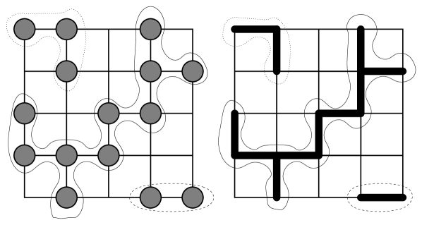
For higher dimensions, much of this picture remains unchanged, although the values of $p_{\rm c}$ and the critical exponents change. The upper critical dimension corresponds to $d=6$ such that mean field theory is valid for $d\geq 6$ with exponents as given in Table 1.

Table 1: Critical exponents $\nu$ and $\beta$ and fractal dimension $D$ for different spatial dimensions. For a more complete list see StaA95 .

Exponent	$d=2$	$d=3$	$d=4$	$d=5$	$d=6-\epsilon$
${\nu}$	$4/3$	$0.88$	$0.68$	$0.57$	$1/2+5\epsilon/84$
$\beta$	$5/36$	$0.41$	$0.64$	$0.84$	$1-\epsilon/7$
$D(p={p_{\rm c}})$	$91/48$	$2.53$	$3.06$	$3.54$	$4-10\epsilon/21$
$D(p<{p_{\rm c}})$	$1.56$	$2$	$12/5$	$2.8$	$-$
$D(p>{p_{\rm c}})$	$2$	$3$	$4$	$5$	$-$

Applications of percolation theory are numerous BunH99 . It is intimately connected to the theory of phase transitions as discussed in Bin97 ; vojta . The connectivity problem is also relevant for diffusion in disordered media schreiber ; kramer and networks grimm . A simple model of forest fires is based on percolation ideas schwabl and even models of stock market fluctuations Voi01 have been devised using ideas of percolation GolLSJ00 . Percolation is therefore a well-established field of statistical physics and it continues its vital progress with more than 230 publications in the cond-mat archives Con93 alone.

2.2 The Coloring Algorithm

As stated above, there are only few exact results available in percolation in $d\geq 2$. Thus in order to proceed further, one has to use computational methods.

The standard numerical algorithm of percolation theory is due to Hoshen and Kopelman HosK76 . Its advantage is due to the fact that it allows to analyze which site belongs to which cluster without having to store the complete lattice. Furthermore, this is being done in one sweep across the lattice, thus reducing computer time.

At the heart of the Hoshen-Kopelman algorithm is a bookkeeping mechanism StaA95 . Look at the site percolation cluster in Fig. 1. Going from left to right and top to bottom through the cluster, we give each site a label (or color) as shown in Fig. 2. If its top or left neighbor is already occupied, then the new site belongs to the same cluster and gets the same label. Otherwise we choose a new label. In this way we can proceed through the cluster until we reach a problem in line 3 as shown in the left column of Fig. 2. According to our above rule the new site, indicated by the bold question mark, can be either $2$ or $4$. This indicates that all sites previously labelled by $2$ and $4$ actually belong to the same cluster. Thus we now introduce an index Id$(\cdot)$ for each cluster label and define it such that the index of a superfluous label, say $4$, points to the right label, viz.  Id$(4)=2$. Proceeding with our analysis into the $4$th row of the lattice, we see in the center column of Fig. 2 that we again have to adjust our index at the position indicated in bold. Instead of labeling this site as $4$, we choose $2\equiv$ Id$(4)$. And consequently, Id$(3)=2$. In this way, we can easily check whether a cluster percolates from top to bottom of the lattice by simply checking whether the label of any occupied site in the bottom row of the lattice has an index equal to any of the labels in the top row. Furthermore, in addition to the top row, we only need to store the row presently under consideration and its predecessor. Thus the storage requirement is linear in lattice size $L$ and not $L^{2}$ as it would be if we were to store the full lattice. Last, the algorithm can also give information about all clusters, say, if needed for a fractal analysis of the non-percolating clusters. A Java implementation of such a coloring algorithm can be found in Ref. Ada97 .

$1$ $1$ $2$ $1$ $2$ $2$ $3$ $4$ ? ${\bullet}$ ${\bullet}$ ${\bullet}$ ${\bullet}$ ${\bullet}$ ${\bullet}$	$1$ $1$ $2$ $1$ $2$ $2$ $3$ $4$ $4$ $3$ $3$ ? ${\bullet}$ ${\bullet}$ ${\bullet}$	$1$ $1$ $2$ $1$ $2$ $2$ $3$ $4$ $4$ $3$ $3$ $2$ ${2}$ $5$ $5$
Id$({1})$ = ${1}$ Id$({2})$ = ${2}$ Id$({3})$ = ${3}$ Id$({4})$ = ${2}$	Id$({1})$ = ${1}$ Id$({2})$ = ${2}$ Id$({3})$ = ${2}$ Id$({4})$ = ${2}$	Id$({1})$ = ${1}$ Id$({2})$ = ${2}$ Id$({3})$ = ${2}$ Id$({4})$ = ${2}$ Id$({5})$ = ${5}$

Figure 2: Schematic description of the Hoshen-Kopelman coloring algorithm of the site percolation problem on a square lattice as shown in Fig. 1. $\bullet$ denotes an occupied site, the numbers denote the cluster labels. The horizontal lines bracket the current and the previous row

2.3 The Growth Algorithm

When we want to study primarily the geometrical properties of percolation clusters, another algorithm is more suitable which allows to generate the desired cluster structure directly. This algorithm is due to Leath Lea76 and works by a cluster-growth strategy. The idea of the algorithm is that we put an occupied site in the center of an otherwise empty lattice. Then we identify its nearest-neighbor sites as shown in Fig. 3. Next we occupy these sites according to the desired percolation probability $p$. We identify the new, yet undecided nearest-neighbor sites, occupy these again with probability $p$ and repeat the procedure. The cluster continues to grow until either all sites at the boundary are unoccupied or the cluster has reached the boundary of the lattice. For $p<p_{\rm c}$, the growth usually stops after a few iterations, while for $p>p_{\rm c}$, percolating clusters are generated almost always. Thus besides giving information about the fractal structure of the percolating clusters, the Leath algorithm can also be used to estimate the value of $p_{\rm c}$. A Java implementation of the Leath algorithm can be found in Refs. KinR98 ; KinR99 .

$\cdot$ $\cdot$ $\cdot$ $\cdot$ $\cdot$ $\cdot$ $\cdot$ $\odot$ $\cdot$ $\cdot$ $\cdot$ $\odot$ ${\bullet}$ $\odot$ $\cdot$ $\cdot$ $\cdot$ $\odot$ $\cdot$ $\cdot$ $\cdot$ $\cdot$ $\cdot$ $\cdot$ $\cdot$

$\cdot$ $\cdot$ $\cdot$ $\cdot$ $\cdot$ $\cdot$ $\cdot$ ${\circ}$ $\odot$ $\cdot$ $\cdot$ ${\circ}$ ${\bullet}$ ${\bullet}$ $\odot$ $\cdot$ $\odot$ ${\bullet}$ $\odot$ $\cdot$ $\cdot$ $\cdot$ $\odot$ $\cdot$ $\cdot$

$\cdot$ $\cdot$ $\cdot$ $\odot$ $\cdot$ $\cdot$ $\cdot$ ${\circ}$ $\bullet$ $\odot$ $\cdot$ ${\circ}$ ${\bullet}$ ${\bullet}$ $\circ$ $\odot$ $\bullet$ ${\bullet}$ $\circ$ $\cdot$ $\cdot$ $\odot$ $\circ$ $\cdot$ $\cdot$

Figure 3: Schematic description of the first three steps in the Leath growth algorithm of the site percolation cluster of Fig. 1. $\bullet$, $\circ$, and $\odot$ denote an occupied, empty, and undecided site

2.4 The Frontier Algorithm

As we have seen in the last section, the outer frontier of the percolation cluster is well defined. The fractal properties of this hull can be measured Vos84 ; ZifCS84 and shown to yield $D_{\rm h}=1.74\pm 0.02$. This suggests yet another algorithm for the determination of $p_{\rm c}$ RosGS85 ; ZifS86 : Generate a lattice with a constant gradient $\nabla p$ of the occupation probability $p$ as shown in Fig. 4.

Figure 4: An example for gradient percolation. All sites at $p=1$ ($p=0$) are occupied (empty). The $15$ large circles correspond to occupied sites. The $8$ light shaded sites belong to the frontier, whereas the $7$ dark shaded sites are part of the interior of the cluster or belong to other clusters. The $5$ small circles correspond to sites in the empty frontier. The dashed line indicates the frontier generating walk. Note that only the $14$ sites with solid circles have actually been visited. The $6$ other circles are shown here just for clarity and need not be generated. According to (2), we have $p_{\rm c}=(8\cdot 0.4375+5\cdot 0.75)/13=0.55769$

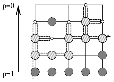
By an algorithm similar to the one used in computing the hull of the percolating cluster, one traverses the frontier of the occupied cluster and determines which sites belong to it and which belong to the empty cluster ZifCS84 ; RosGS85 ; ZifS86 . Then a very reliable estimate for the percolation threshold can be computed as

$$p_{\rm c}=\frac{N_{\rm o}p_{\rm co}+N_{\rm e}p_{\rm ce}}{N_{\rm o}+N_{\rm e}},$$ (2)

where $N_{o,e}$ denotes the number of sites in the occupied (empty) frontier and $p_{co,ce}$ is the mean height of the associated frontiers, respectively. Note that instead of actually generating the percolation lattice, the algorithm instead proceeds by just generating the sites needed for the construction of the frontier. Thus instead of dealing with, say, ${\cal O}(L^{2})$ sites as in the Hoshen-Kopelman and Leath algorithms for a lattice in $d=2$, one only needs ${\cal O}(L)$ sites in the present algorithm frontier . This reduces computer time and estimates for $p_{\rm c}$ in a large variety of lattices can be obtained with high accuracy SudZ99 ; SykE63 ; ZifS97 ; LorZ98 ; KleZ98 ; NewZ00 as shown in Table 2.

Table 2: Various current estimates of $p_{\rm c}$ for site and bond percolation on different lattices in $d=2$ SudZ99 ; SykE63 ; ZifS97 ; LorZ98 ; KleZ98 ; NewZ00 . Exactly known values are emphasized. The lattices are classified according to their number of first, second and more nearest-neighbors. The upper index gives the corresponding number in the dual lattice

lattice		site ${p_{\rm c}}$	bond ${p_{\rm c}}$
$3,12^{2}$		0.807 904
$4,6,12$		$0.747\,806$
$4,8^{2}$		$0.729\,724$
$6^{3}$	honeycomb	$0.697\,043$	0.652 703
$3,6,3,6$	Kagomé	0.652 703	$0.524\,4$
$4^{4}$	dice	$0.584\,8$	$0.475\,4$
$3,4,6,4$		$0.621\,819$
$4^{4}$	square	$0.592\,746\,0$	0.500 000
$3^{4},6$		$0.579\,498$
$3^{2},4,3,4$		$0.550\,806$
$3^{3},4^{2}$		$0.550\,213$
$3^{6}$	triangular	0.500 000	0.347 296

3 Real-Space Renormalization

3.1 Making Use of Self-Similarity

As mentioned in Sect.  2, the transition at $p_{\rm c}$ corresponds to a second-order phase transition and the correlation length $\xi$ is infinite. There is no particular length scale in the system and all clusters are statistically similar to each other. This self-similarity schreiber is at the bottom of the renormalization description just as for the fractal analysis of the percolation clusters.

We may use the self-similarity in the following way. Let us replace a suitable collection of sites by super-sites and then study percolation of the super-lattice HarLHD75 ; ReyKS77 ; Ber78 ; ReySK80 ; EscSH81 . In general, the occupation probability $p^{\prime}$ of the super-lattice will be different from the original $p$. Furthermore, if the extent of the collection of sites in the lattice was $b$, then the super-lattice will have a lattice constant $b$. Thus $\xi=b\xi^{\prime}$ and with $\xi\propto|p-p_{\rm c}|^{-\nu}$, we find

$$b|p^{\prime}-p_{\rm c}|^{-\nu}\equiv|p-p_{\rm c}|^{-\nu}$$ (3)

and consequently,

$$\nu=\frac{\log b}{\log\frac{\mathrm{d}p^{\prime}}{\mathrm{d}p}}.$$ (4)

As an example, let us consider the bond percolation problem on a square lattice ReyKS77 ; Ber78 ; ReySK80 . Here we replace 5 bonds by a super-bond in the horizontal direction as shown in Fig. 5.

Figure 5: The possible combinations of bonds (thin lines) that lead to a super-bond (thick line) together with their respective probabilities for bond percolation on a square lattice

Summing all probabilities for a connected, horizontal super-bond as shown in Fig. 5, we find that

$$p^{\prime}=p^{5}+5p^{4}(1-p)+8p^{3}(1-p)^{2}+2p^{2}(1-p)^{3}.$$ (5)

At the transition, we have $p^{\prime}=p$ and thus (5) has the solutions $p=0$, $0.5$, and $1$. The first and last solution correspond to a completely empty or occupied lattice and are trivial. The second solution reproduces the exact result of Table 2. From 4), we compute $\nu=1.4274$ which is already within $8\%$ of the exact result $4/3$. Thus the real-space RG scheme gives very good approximations to the known results. But beware, it may not always be that simple: the reader is encouraged to devise a similar RG scheme for site percolation on a square lattice.

3.2 Monte-Carlo RG

The scheme of the last section is approximate since it cannot correctly handle situations like the one in Fig. 6. In order to improve, we can construct an RG scheme that uses a larger collection of bonds. The total number of (connected and unconnected) configurations in such a collection of $n$ bonds is $2^{n}$, putting severe bounds on the practicability of the approach for analytic calculations. However, the task is ideally suited for computers. On the CD accompanying this book, I include a set of Mathematica routines that compute the real-space RG for a $d=2$ triangular lattice.

Figure 6: Although the original bonds (thin lines) are not connected, the RG procedure outlined in the text nevertheless leads to two connected horizontal super-bonds (thick lines)

4 The Quantum-Hall Effect

In 1980, von Klitzing et al. KliDP80 found that the Hall resistance $R_{\rm H}$ of MOSFETs at strong magnetic field $B$ exhibits a step-like behavior which is accompanied with a simultaneously vanishing longitudinal resistance $R$. This is in contrast to the classical Hall effect which gives a linear dependence of $R_{\rm H}$ on $B$. Even more surprising, the values of $R_{\rm H}$ at the transitions are given by universal constants, i.e., $\frac{1}{i}\frac{h}{e^{2}}$, where $i$ is an integer.

Since its discovery this so-called integer quantum Hall effect (IQHE) was studied extensively JanVFH94 ; ChaP95 . Besides semi-phenomenological models simply assuming a localization-delocalization transition more general theories considered, e.g., gauge invariance Lau81 , topological quantization ThoKNN82 , scattering Pra81 and field theoretical approaches Pru84 .

4.1 Basics of the IQHE

A simple understanding of the IQHE can be gained by considering the Hamiltonian of a single electron in a magnetic field,

$$H_{0}=\frac{1}{2m}\left({\bf p}+\frac{e}{c}{\bf A}\right)^{2}=\frac{\hbar\omega_{\rm c}}{2l_{B}^{2}}\left(\xi^{2}+\eta^{2}\right).$$ (6)

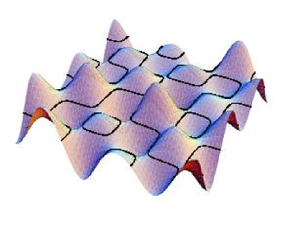
where $\vec{A}$ denotes the vector potential and the Hamiltonian has been rewritten in guiding center coordinates $X=x-\zeta$, $Y=y-\eta$ and relative coordinates $\zeta$, $\eta$ Lan30 . Here, $\omega_{\rm c}=\frac{eB}{m}$ is the frequency of the classical cyclotron motion and $l_{B}=(\frac{\hbar}{eB})^{1/2}$ is the radius of the cyclotron motion. The spectrum of this Hamiltonian is simply the harmonic oscillator with $E_{n}=\left(n+\frac{1}{2}\right)\hbar\omega_{\rm c},$ $n=0$, $1$, $\ldots$. These Landau levels are infinitely degenerate since the Hamiltonian no longer contains $X$ and $Y$. Thus the spectrum consists of $\delta$-function peaks as indicated in Fig. 7. Introducing disorder into the model by adding a smooth random potential $V(\vec{r})$ in (6) results in drift motion of the guiding center

$$\dot{X}=\frac{{\rm i}}{\hbar}\left[H,X\right]=\frac{l_{B}^{2}}{\hbar}\frac{\partial V}{\partial y},\quad\dot{Y}=\frac{{\rm i}}{\hbar}\left[H,Y\right]=-\frac{l_{B}^{2}}{\hbar}\frac{\partial V}{\partial x}.$$ (7)

perpendicular to the gradient of $V(\vec{r})$ (see Fig. 8). Furthermore, the degeneracy of the Landau levels is lifted, the $\delta$-function density of states broadens JanVFH94 , giving rise to a band-like structure as shown in Fig. 7. If the sample is penetrated by a strong magnetic field, the cyclotron motion is much smaller than the potential fluctuations. Consequently, the electron motion can be separated into cyclotron motion and motion of the guiding center along equipotential lines of the energy landscape.

Figure 7: Density of states (DOS), transversal and longitudinal conductivity as a function of $E_{\rm F}$ or, equivalently, filling factor $\nu_{\rm f}$ or $B^{-1}$ ChaP95 . The peak in the middle of the band represents one $\delta$-function peak of the clean Landau model. Dark shaded regions of the density of states correspond to localized states. The thin dashed line (with non-zero slope) for $\sigma_{xy}$ indicates the classical Hall result

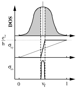
The IQHE can then be understood as follows: assume that the center of the broadened Landau levels contain extended states that can support transport, whereas the other states are spatially localized and cannot. This is similar to the standard picture in the theory of Anderson localization schreiber ; kramer . Changing the Fermi energy $E_{\rm F}$ or the filling factor $\nu_{\rm f}=2\pi l_{B}^{2}\rho_{\rm e}=2\pi\hbar\rho_{\rm e}/eB\propto E_{\rm F}$, where $\rho_{\rm e}$ denotes the electron density, we first have $E_{\rm F}$ in the region of localized states and both $\sigma_{xx}$ and $\sigma_{xy}$ are $0$. When $E_{\rm F}$ reaches the region of extended states, there is transport, $\sigma_{xx}$ is finite and $\sigma_{xy}=e^{2}/h$. Next, $E_{\rm F}$ again reaches a region of localized states and $\sigma_{xx}$ drops back to $0$ until we reach the extended states in the next Landau level.

This picture suggests the following effective classical high-field model Ior82 of the IQHE: Neglecting the cyclotron motion (i.e., large $B$) and quantum effects (i.e., only one extended state) the classical electron transport with energy $E_{\rm F}$ through the sample only depends on the “height” of the saddle points in the potential energy landscape $V(\vec{r})$. One obtains a classical bond-percolation problem StaA95 , in which saddle points are mapped onto bonds. A bond is connecting only when the potential of the corresponding saddle point equals the energy of the electron $E_{\rm F}$. From percolation theory follows StaA95 that an infinite system is conducting only when $E_{\rm F}=\langle V\rangle$. Using this model one could already describe the localization-delocalization transition and thus the quantized plateaus in resistivity observed in IQHE JanVFH94 . But for bond percolation the correlation length diverges at the transition with an exponent of $\nu=4/3$ which is in contrast to the value found in the QH experiments.

4.2 RG for the Chalker-Coddington Network Model

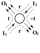
The Chalker-Coddington (CC) network model improved the high-field model by introducing quantum corrections ChaC88 , namely tunneling and interference. Tunneling occurs, in a semiclassical view, when electron orbits come close enough to each other and the electron cyclotron motions overlap. This happens at the saddle points, which now act as quantum scatterers connecting two incoming with two outgoing channels by a scattering matrix as shown in Fig. 8.

Figure 8: Left: Schematic plot of a smooth random potential $V(\vec{r})$ with equipotential lines at $E=\langle V\rangle$ indicated in black. Right: Equipotential lines of the same potential for $E=\langle V\rangle-E_{\rm max}/2$, $\langle V\rangle$, and $\langle V\rangle+E_{\rm max}/2$ corresponding to long dashed, solid and short dashed lines. Note the solid line percolating the system from top to bottom as indicated by the arrows

Similar to bond percolation a network can be constructed such that the saddle points are mapped onto bonds. While moving along an equipotential line an electron accumulates a random phase which reflects the disorder of $V(\vec{r})$. Results for this quantum percolation also show one extended state in the middle of the Landau band. The critical properties at the transition, especially the value of the exponent $\nu\approx 2.4$ LeeWK93 , agree with experiments KocHKP91 ; SchVOW00 .

Figure 9: Left: A single saddle point (circle) connected to incoming and outgoing currents $I_{i}$, $O_{i}$ via transmission and reflection amplitudes $t$ and $r$. Right: A network of $5$ saddle points can be renormalized into a single super-saddle point by an RG approach very similar to the bond percolation problem of Sect.  3. The phases are schematically denoted by the $\phi$’s

As explained for the bond percolation problem we now apply the RG method to the CC model. The RG structure which builds the new super-saddle points is displayed in Fig. 9. It consists of $5$ saddle points drawn as bonds. The links (and phase factors) connecting the saddle points are indicated by arrows pointing in the direction of the electron motion due to the magnetic field. Each saddle point acts as a scatterer connecting the $2$ incoming $I_{1,2}$ with the $2$ outgoing channels $O_{1,2}$

$$\left(\begin{array}[]{c}O_{1}\\ O_{2}\end{array}\right)=\left(\begin{array}[]{cc}t_{i}&r_{i}\\ r_{i}&-t_{i}\end{array}\right)\left(\begin{array}[]{c}I_{1}\\ I_{2}\end{array}\right)$$ (8)

with reflection coefficients $r_{i}$ and transmission coefficients $t_{i}$, which are assumed to be real numbers. The complex phase factors enter later via the links between the saddle points. By this definition – including the minus sign – the unitarity constraint $t_{i}^{2}+r_{i}^{2}=1$ is fulfilled a priori. The amplitude of transmission of the incoming electron to another equipotential line and the amplitude of reflection and thus staying on the same equipotential line add up to unity – electrons do not get lost.

In order to obtain the scattering equation of the super-saddle point we now need to connect the $5$ scattering equations according to Fig. 9. For each link the amplitude of the incoming channels is defined by the amplitude of the outgoing channel of the previous saddle point multiplied by the corresponding complex phase factor $\mathrm{e}^{{\rm i}\phi_{k}}$. This results in a system of $5$ matrix equations, which has to be solved. One obtains an RG equation for the transmission coefficient $t^{\prime}$ of the super-saddle point GalR97 analogously to Eq. (5),

$$t^{\prime}=\frac{t_{15}(r_{234}\mathrm{e}^{{\rm i}\phi_{2}}-1)+t_{24}\mathrm{e}^{{\rm i}(\phi_{3}+\phi_{4})}(r_{135}\mathrm{e}^{-{\rm i}\phi_{1}}-1)+t_{3}(t_{25}\mathrm{e}^{{\rm i}\phi_{3}}+t_{14}\mathrm{e}^{{\rm i}\phi_{4}})}{(r_{3}-r_{24}\mathrm{e}^{{\rm i}\phi_{2}})(r_{3}-r_{15}\mathrm{e}^{{\rm i}\phi_{1}})+(t_{3}-t_{45}\mathrm{e}^{{\rm i}\phi_{4}})(t_{3}-t_{12}\mathrm{e}^{{\rm i}\phi_{3}})}$$ (9)

depending on the products $t_{i\ldots j}=t_{i}\cdot\ldots\cdot t_{j}$, $r_{i\ldots j}=r_{i}\cdot\ldots\cdot r_{j}$ of transmission and reflection coefficients $t_{i}$ and $r_{i}$ of the $i=1,\ldots,5$ saddle points and the $4$ random phases $\phi_{k}$ accumulated along equipotentials in the original lattice. For further algebraic simplification one can apply a useful transformation of the amplitudes $t_{i}=(\mathrm{e}^{z_{i}}+1)^{-1/2}$ and $r_{i}=(\mathrm{e}^{-z_{i}}+1)^{-1/2}$ to heights $z_{i}$ relative to heights $V_{i}$ of the saddle points. The conductance $G$ is connected to the transmission coefficient $t$ by $G=|t|^{2}e^{2}/h$ ButILP85 .

4.3 Conductance Distributions at the QH Transition

For the numerical determination of the conductance distribution, we first choose an initial probability distribution $P_{0}$ of transmission coefficients $t$. The distribution is discretized in at least $1000$ bins. Thus the bin width is typically $0.001e/\sqrt{h}$ for the interval $t\in[0,e/\sqrt{h}]$.

Using the initial distribution $P_{0}(t)$, we now randomly select many different transmission coefficients and insert them into the RG equation (9). Furthermore, the phases $\phi_{j}$, $j=1,\ldots 4$ are also chosen randomly, but according to a uniform distribution $\phi_{j}\in[0,2\pi]$. By this method at least $10^{7}$ super-transmission coefficients $t^{\prime}$ are calculated and their distribution $P_{1}(t^{\prime})$ is stored. Next, $P_{1}$ is averaged using a Savitzky-Golay smoothing filter PreFTV92 in order to decrease statistical fluctuations. This process is then repeated using $P_{1}$ as the new initial distribution.

Figure 10: Conductance distribution at a QH plateau-to-plateau transition. The squares correspond to the fixed-point distribution, dashed and dot-dashed lines to the initial distribution and an unstable distribution, respectively. The solid line indicates a fit of the FP distribution $P_{\rm c}(t)$ by three Gaussians. Inset: Moments of the FP distribution $P_{\rm c}(G)$. The dashed lines indicate various predictions based on extrapolations of results for small $m$ WanJL96 . The dotted line denotes the moments of a constant distribution

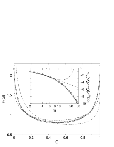
The iteration process is stopped when the distribution $P_{i}$ is no longer distinguishable from its predecessor $P_{i-1}$ and we have reached the desired fixed-point (FP) distribution $P_{\rm c}(t)$. However, due to numerical instabilities, small deviations from symmetry add up such that typically after $15$–$20$ iterations the distributions become unstable and converge towards the classical FPs of no transmission or complete transmission similar to the classical percolation case. Figure 10 shows this behavior for one of the RG iterations. The FP distribution $P_{\rm c}(G)$ shows a flat minimum around $G=0.5e^{2}/h$ and sharp peaks at $G=0$ and $G=e^{2}/h$. It is symmetric with $\langle G\rangle=0.498e^{2}/h$. This is in agreement with previous theoretical WeyJ98 ; AviBB99 and experimental CobK96 results whereas our results contain much less statistical fluctuations. Furthermore we determine moments $\langle(G-\langle G\rangle)^{m}\rangle$ of the FP distribution $P_{\rm c}(G)$. As shown in Fig. 10 for small moments up to $m=6$ our results agree with the work of Wang et al. WanJL96 , who computed moments $m\leq 8.5$. But more interesting is the fact that the obtained moments of the FP distribution can hardly be distinguished from the moments of a simple constant distribution thus indicating the influence of the broad flat minimum of the FP distribution around $G=0.5e^{2}/h$.

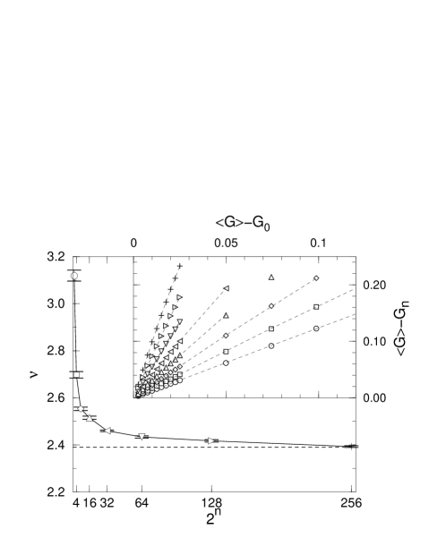
For the determination of the critical exponent, we next perturb the FP distribution slightly, i.e., we construct a distribution with shifted average $G_{0}$. Then we perform an RG iteration and compute the new average $G_{1}$ of $P_{1}(G)$. Tracing the shift of the perturbed average $G_{n}$ for several initial shifts $G_{0}$, we expect to find a linear dependence of $G_{n}$ on $G_{0}$ for each iteration step $n$. The critical exponent is then related to the slope $\mathrm{d}G_{n}/\mathrm{d}G_{0}$ CaiRRS00 . Figure 11 shows the resulting $\nu$ in dependence on the iteration step and thus system size. The curve converges close to $\nu\approx 2.4$, i.e. the value obtained by Lee et al. LeeWK93 . Note that the “system size” is more properly called a system magnification, since we start the RG iteration with an FP distribution valid for an infinite system and then magnify the system in the course of the iteration by a factor $2^{n}$.

Figure 11: Critical exponent $\nu$ as a function of magnification factor $2^{n}$ for RG step $n$. The dashed line shows the expected result $\nu=2.39$. Inset: The shift of the average $G_{n}$ of $P(G)$ is linear in $G_{0}$. The dashed lines indicate linear fits to the data

5 Summary and Conclusions

The percolation model represents the perhaps simplest example of a system exhibiting complex behavior although its constituents – the sites and bonds – are chosen completely uncorrelated. Of course, the complexity enters through the connectivity requirement for percolating clusters. I have reviewed several numerical algorithms for quantitatively measuring various aspects of the percolation problem. The specific choice reflects purely my personal preferences and I am happy to note that other algorithms such as breadth- and depth-first algorithms AhoHU83 have been introduced by P. Grassberger in his contribution grassberger .

The real-space RG provides an instructive use of the underlying self-similarity of the percolation model at the transition. Furthermore, it can be used to study very large effective system sizes. This is needed in many applications. As an example, I briefly reviewed and studied the QH transition and computed conductance distributions, moments and the critical exponent. These results can be compared to experimental measurements and shown to be in quite good agreement.

References

- (1) We note that the WEH-Ferienkurs, following which this article has been prepared, took place during early fall.
- (2) S.R. Broadbent, J.M. Hammersley: Proc. Camb. Philos. Soc. 53, 629 (1957)
- (3) J.M. Hammersley: Proc. Camb. Philos. Soc. 53, 642 (1957)
- (4) J.M. Hammersley: Ann. Math. Statist. 28, 790 (1957)
- (5) D. Stauffer, A. Aharony: Perkolationstheorie (VCH, Weinheim 1995)
- (6) For any finite lattice, “infinite” means a cluster that reaches from top to bottom and/or left to right through the lattice.
- (7) M. Schreiber, F. Milde (this volume).
- (8) K. Binder: Rep. Prog. Phys. 60, 487 (1997)
- (9) G. Grimmett: Percolation (Springer, Berlin 1989)
- (10) A. Bunde, S. Havlin (Eds.): Percolation and Disordered Systems: Theory and Applications (North-Holland, Amsterdam 1999)
- (11) T. Vojta, (this volume).
- (12) B. Kramer, (this volume).
- (13) U. Grimm, (this volume).
- (14) K. Schenk, B. Drossel, F. Schwabl, (this volume).
- (15) J. Voit: The Statistical Mechanics of Capital Markets (Springer, Heidelberg 2001)
- (16) J. Goldenberg, B. Libai, S. Solomon, N. Jan, D. Stauffer: Marketing Percolation (2000). Cond-mat/9905426
- (17) http://de.arXiv.org/, 1993–2000
- (18) J. Hoshen, R. Kopelman: Phys. Rev. B 14, 3438 (1976)
-
(19)
C. Adami: (1997),
http://www.krl.caltech.edu/~adami/CD1/Percolation/percolation.html, likely to change without prior notice - (20) P. Leath: Phys. Rev. B 14, 5056 (1976)
- (21) W. Kinzel, G. Reents: Physics by Computer (Springer, Berlin 1998)
(22)
W. Kinzel, G. Reents: (1999),
http://wptx15.physik.uni-wuerzburg.de/TP3/applet_java/percgr.html, likely to change without prior notice - (23) R.F. Voss: J. Phys. A: Math. Gen. 17(7), L373 (1984)
- (24) R.M. Ziff, P.T. Cummings, G. Stell: J. Phys. A: Math. Gen. 17, 3009 (1984)
- (25) M. Rosso, J.F. Gouyet, B. Sapoval: Phys. Rev. B 32, 6053 (1985)
- (26) R.M. Ziff, B. Sapoval: J. Phys. A: Math. Gen. 19, L1169 (1986)
- (27) Alas, this intuitively convincing argument is not strictly true: The percolation frontier is a fractal and as such scales Vos84 . On the other hand, it is not the random number generation for sites in the Hoshen-Kopelman algorithm but rather the numerical determination of the percolating clusters which is numerically challenging.
- (28) P.N. Suding, R.M. Ziff: Phys. Rev. E 60, 275 (1999)
- (29) M.F. Sykes, J.W. Essam: Phys. Rev. Lett. 10, 3 (1963)
- (30) R.M. Ziff, P.N. Suding: J. Phys. A: Math. Gen. 30, 5351 (1997)
- (31) C.D. Lorenz, R.M. Ziff: Phys. Rev. B 57, 230 (1998)
- (32) P. Kleban, R.M. Ziff: Phys. Rev. B 57, R8075 (1998)
- (33) M.E.J. Newman, R.M. Ziff: (2000). Cond-mat/0005264
- (34) A.B. Harris, T.C. Lubensky, W.K. Holcomb, C. Dasgupta: Phys. Rev. Lett. 35, 327 (1975)
- (35) P.J. Reynolds, W. Klein, H.E. Stanley: J. Phys. C: Solid State Phys. 10, L167 (1977)
- (36) J. Bernasconi: Phys. Rev. B 18, 2185 (1978)
- (37) P.J. Reynolds, H.E. Stanley, W. Klein: Phys. Rev. B 21, 1223 (1980)
- (38) P.D. Eschbach, D. Stauffer, H. Herrmann: Phys. Rev. B 23, 422 (1981)
- (39) K.v. Klitzing, G. Dorda, M. Pepper: Phys. Rev. Lett. 45, 494 (1980)
- (40) M. Janssen, O. Viehweger, U. Fastenrath, J. Hajdu: Introduction to the Theory of the Integer Quantum Hall effect (VCH, Weinheim 1994)
- (41) T. Chakraborty, P. Pietilänen: The Quantum Hall effects (Springer, Berlin 1995)
- (42) R.B. Laughlin: Phys. Rev. B 23, 5632 (1981)
- (43) D.J. Thouless, M. Kohmoto, M.P. Nightingale, M. den Nijs: Phys. Rev. Lett. 49, 405 (1982)
- (44) R.E. Prange: Phys. Rev. B 23, 4802 (1981)
- (45) A.M.M. Pruisken: Nucl. Phys. B 235, 277 (1984)
- (46) D.L. Landau: Z. Phys. 64, 629 (1930)
- (47) S.V. Iordanskii: Solid State Commun. 43, 1 (1982)
- (48) J.T. Chalker, P.D. Coddington: J. Phys.: Condens. Matter 21, 2665 (1988)
- (49) D.H. Lee, Z. Wang, S. Kivelson: Phys. Rev. Lett. 70, 4130 (1993)
- (50) S. Koch, R.J. Haug, K. v. Klitzing, K. Ploog: Phys. Rev. B 43, 6828 (1991)
- (51) R.T.F. van Schaijk, A. de Visser, S.M. Olsthoorn, H.P. Wei, A.M.M. Pruisken: Phys. Rev. Lett. 84, 1567 (2000)
- (52) A.G. Galstyan, M.E. Raikh: Phys. Rev. B 56, 1422 (1997)
- (53) M. Büttiker, Y. Imry, R. Landauer, S. Pinhas: Phys. Rev. B 31, 6207 (1985)
- (54) W.H. Press, B.P. Flannery, S.A. Teukolsky, W.T. Vetterling: Numerical Recipes in FORTRAN, 2nd edn. (Cambridge University Press, Cambridge 1992)
- (55) Z. Wang, B. Jovanovic, D.H. Lee: Phys. Rev. Lett. 77, 4426 (1996)
- (56) A. Weymer, M. Janssen: Ann. Phys. (Leipzig) 7, 159 (1998). Cond-mat/9805063
- (57) Y. Avishai, Y. Band, D. Brown: Phys. Rev. B 60, 8992 (1999)
- (58) D.H. Cobden, E. Kogan: Phys. Rev. B 54, R17 316 (1996)
- (59) P. Cain, R.A. Römer, M.E. Raikh, M. Schreiber: Localization-Delocalization quantum Hall transition in the present of a quenched disorder (2001).
- (60) A. Aho, J.E. Hopcroft, J.D. Ullman: Data Structures and Algorithms (Addison-Wesley, New York 1983)
- (61) P. Grassberger, (this volume).
Index
- bin width §4.3
- bond §4.1
- bond percolation §3.1, §4.1
- bonds §2.1
- CC §4.2
- CC network model §4.2
- Chalker-Coddington network model §4.2
- chessboard §1
- conductance §4.2
- connectivity §2.1, §2.1
- correlation function §2.1
- correlation length §2.1
- critical exponent §2.1, §4.3
- cyclotron motion §4.1
- disorder §4.1
- drift motion §4.1
- equipotential lines §4.1
- extended states §4.1
- Fermi energy §4.1
- filling factor §4.1
- finite-size scaling §2.1
- fixed-point §4.3
- fixed-point distribution §4.3
- FP §4.3
- FP distribution §4.3
- fractal §2.1, §3.1
- frontier §2.4, §2.4
- growth §2.3
- growth algorithm Figure 3
- guiding center §4.1
- Hall resistance §4
- high field model §4.1
- Hoshen-Kopelman algorithm §2.2
- hull of the percolating cluster §2.4
- index of labels §2.2
- Indian summer §1
- infinite cluster §2.1, §2.1, §2.1
- integer quantum Hall effect §4
- interference §4.2
- IQHE §4
- Landau level §4.1
- Landau levels §4.1
- leaf §2.1
- Leath algorithm §2.3
- leaves §2.1
- localized §4.1
- longitudinal resistance §4
- magnetic field §4.1
- mean field theory §2.1
- moments of the FP distribution §4.3
- occupation probability §3.1
- percolation probability §2.3
- percolation threshold §2.1, §2.1
- quantum percolation §4.2
- real-space renormalization group §1
- reflection coefficients §4.2
- renormalization §3.1
- RG §1, §3.1, §3.2, §4.2, §5
- RG equation §4.2, §4.3
- RG iteration §4.3
- RG iterations §4.3
- Savitzky-Golay smoothing §4.3
- second order phase transition §2.1
- self-similarity §3.1, §3.1, §5
- site percolation §2.1
- sites §2.1
- storage requirement §2.2
- super-bond §3.1
- theory of phase transitions §2.1
- transmission coefficients §4.2
- tunneling §4.2
- unitarity §4.2
- universality §2.1
- upper critical dimension §2.1
- vector potential §4.1