Persistence in the One-Dimensional $A+B\rightarrow\emptyset$ Reaction-Diffusion Model

Abstract

The persistence properties of a set of random walkers obeying the $A+B\rightarrow\emptyset$ reaction, with equal initial density of particles and homogeneous initial conditions, is studied using two definitions of persistence. The probability, $P(t)$, that an annihilation process has not occurred at a given site has the asymptotic form $P(t)\sim{\rm const}+t^{-\theta}$, where $\theta$ is the persistence exponent (“type I persistence”). We argue that, for a density of particles $\rho\gg 1$, this non-trivial exponent is identical to that governing the persistence properties of the one-dimensional diffusion equation, $\partial_{t}\phi=\partial_{xx}\phi$, where $\theta\simeq 0.1207$ [1]. In the case of an initially low density, $\rho_{0}\ll 1$, we find $\theta\simeq 1/4$ asymptotically. The probability that a site remains unvisited by any random walker (“type II persistence”) is also investigated and found to decay with a stretched exponential form, $P(t)\sim\exp(-{\rm const}\times\rho_{0}^{1/2}t^{1/4})$, provided $\rho_{0}\ll 1$. A heuristic argument for this behavior, based on an exactly solvable toy model, is presented.

I Introduction

Diffusion-limited reactions are used to model a wide range of phenomena in physics, chemistry and biology, and continue to stimulate current research. Reaction-diffusion processes have been applied to studies such as stochastic spin-flip dynamics , exciton-exciton dynamics in tetra-methylammonium manganese trichloride [3], the kinetics of bipolymerisation [4], reptation of DNA in gels [5], interface growth [6], diffusion of zeolites [7] and other phenomena such as competing species in biology, self-organised criticality, pattern formation and dynamic phase transitions.

Much of the effort to date has focused on reactions of the form $A+A\rightarrow\emptyset$ and $A+B\rightarrow\emptyset$, with a variety of boundary and initial conditions . It is well appreciated that within the context of these models there exists an upper critical dimension $d_{c}$, below which spatial fluctuations in the initial distribution of the reactants play a significant role in the evolution of the density of the particles. This dependence on the microscopic fluctuations invalidates traditional approaches such as the mean-field approximation. Attempts to understand the role played by fluctuations have involved numerous techniques, including Smoluchowski-type approximations [8] and field-theoretic methods [9, 10, 11]. In this paper we set out to elucidate the effects of these fluctuations on persistence within the context of the $A+B\rightarrow\emptyset$ model.

Persistence phenomena have received considerable attention in recent years [1, 12, 13, 14, 15, 16, 17, 18, 19, 20, 21, 22, 23]. Theoretical and computational studies include spin systems in one [12, 14] and higher [15] dimensions, diffusion fields [1, 16], fluctuating interfaces [17] and phase ordering dynamics [18]. Experimental studies include the coarsening dynamics of breath figures [19], soap froths [20] and twisted nematic liquid crystals [21]. Persistence in nonequilibrium critical phenomena has also been studied in the context of the global order parameter $M(t)$ regarded as a stochastic process [22]. Reaction-diffusion models offer much scope for the study of persistence and have already contributed significantly to our understanding in this area [23].

The definition of persistence is as follows. Let $\phi(x,t)$ be a stochastic variable fluctuating in space and time according to some dynamics. The persistence probability is simply the probability $P(t)$ that at a fixed point in space, the quantity ${\rm sgn}\,[\phi(x,t)-\langle\phi(x,t)\rangle]$ does not change up to time $t$. In many systems of physical interest a power law decay, $P(t)\sim t^{-\theta}$, is observed, where $\theta$ is the persistence exponent and is, in general, nontrivial. The nontriviality of $\theta$ emerges as a consequence of the coupling of the field $\phi(x,t)$ to its neighbours, since such coupling implies that the stochastic process at a fixed point in space and time is non-Markovian.

Two distinct types of persistence emerge naturally in the study of the $A+B\rightarrow\emptyset$ reaction-diffusion model. Consider a nonequilibrium field $\phi(x,t)$ which takes values at each lattice site $x$. The field evolves in time $t$ through interactions with its neighbours. In type I persistence, the field $\phi(x,t)$ changes its sign whenever an event occurs at the lattice site $x$ at time $t$, where an event is defined to be the reaction process $A+B\rightarrow\emptyset$. Type II persistence satisfies the conventional definition and the field $\phi(x,t)$ changes sign when the lattice site $x$ is visited by either an $A$ or $B$ particle at time $t$. The persistence probability at time $t$ is defined as the fraction of sites in which the stochastic field $\phi(x,t)$ did not change its value in the time interval $[0,t]$. Our analysis suggests, in the case of type I persistence, that when the initial density of particles is high ($\rho_{0}\gg 1$, where $\rho_{0}$ is the density of either $A$ or $B$ particles), the value of the persistence exponent is identical to that which emerges in the study of the one-dimensional diffusion equation $\partial_{t}\phi=\partial_{xx}\phi$, as long as the running density, $\rho(t)$, satisfies $\rho(t)\gg 1$. This yields $\theta\simeq 0.1207$ [1]. When, however, the initial density of particles is low ($\rho_{0}\ll 1$), we find $\theta\simeq 1/4$, in agreement with a simple heuristic argument based on the decay of the density. In the case of type II persistence we show that the persistence decays with the “stretched exponential” form $P(t)\sim\exp(-{\rm const}\times\rho_{0}^{1/2}t^{1/4})$, and we provide a heuristic derivation of this based on the behavior of a toy model.

The paper is organised as follows. In section I we introduce the model and calculate the evolution of the particle density for all $\rho_{0}$, including $\rho_{0}\gg 1$. In section II we present our results for type I persistence. In section III we introduce a generalised toy model of noninteracting diffusing particles and illuminate, through a special case, the type II persistence properties of the $A+B\rightarrow\emptyset$ model. All our predictions are tested by extensive numerical simulations.

II PARTICLE DENSITY IN THE $A+B\rightarrow\emptyset$ model

We are concerned with the following model. Consider the $A+B\rightarrow\emptyset$ reaction involving two types of particle, both executing diffusive random walks. The particles move on a one-dimensional lattice with periodic boundary conditions, and react upon contact to form an inert particle. At $t=0$, exactly equal numbers, $N_{A}(0)=N_{B}(0)$, of $A$ particles and $B$ particles are randomly distributed on the lattice. This is done by randomly assigning one half of the lattice sites to $A$ particles and the other half to $B$-particles. The $A$-sites and $B$-sites are then randomly filled with $A$ and $B$ particles, i.e. each $A(B)$-particle occupies each of the $A(B)$-sites with equal probability such that, at large scales, both densities $\rho_{A}(0)$ and $\rho_{B}(0)$ are initially homogeneous. We define $\rho_{0}=\rho_{A}(0)=\rho_{B}(0)=N_{A}(0)/L$ where $L$ is the size of the lattice. The two species are also given the same diffusion constant $D_{A}=D_{B}=D=1/2$. Our model then evolves permitting multiple occupancy of sites, but we impose an instantaneous reaction so that each lattice site contains only one type of particle.

The mean-field approach yields an asymptotic decay of the particle density according to $\rho_{A}(t)=\rho_{B}(t)\sim{\rm const}\times t^{-1}$ with an amplitude independent of the initial density. However, in low enough spatial dimension, $d\leq d_{c}=4$, the dominating process asymptotically is the diffusive decay of the fluctuations in the initial conditions. This leads to anomalous kinetics and it was shown by Toussaint and Wilczek [24] that

$$\left<\rho_{A}(t)\right>=\left<\rho_{B}(t)\right>\sim\frac{\sqrt{\rho}_{0}}{\pi^{1/2}(8\pi)^{d/4}}(Dt)^{-d/4}\ .$$ (1)

This result has been confirmed using field-theoretic methods for $2<d<4$ by Lee and Cardy [10]. The exponent $-d/4$ has also been rigorously confirmed by Bramson and Lebowitz [25]. The numerical simulations which have been performed in one [24, 26], two [24, 27] and three dimensions [28] are also in good agreement with the analytical predictions of the decay exponent. However, it was noted by Lee and Cardy [10] that, although in one dimension reasonable agreement with the dependence on the initial density has been found, in higher dimensions the $\sqrt{\rho(0)}$ amplitude dependence has not been observed. They suggest that, in the one-dimensional simulations, the initial average occupation number per site was kept low, whereas for the higher dimensional simulations it was necessary to start with a nearly full lattice in order to reach the asymptotic regime and therefore that Eq. (1) might not be a universal result, but rather a limit for small initial density. We believe this to be the case. We focus on the particle density in one dimension. In our study of type I persistence we are particularly interested in the limit of high initial particle density, $\rho_{0}\gg 1$, where the problem should map onto simple diffusion. As a precursor to looking at the persistence, therefore, we first consider how the particle density decays with time in this limit.

In the high-density limit, where there are many particles per site, one can neglect dynamical fluctuations in the density. If $N_{n}(t)$ is the number of particles at site $n$ at time $t$, the dynamics of $N_{n}(t)$ is governed by diffusion:

$$\dot{N}_{n}(t)=D(N_{n+1}(t)-2N_{n}(t)+N_{n-1}(t))\ .$$ (2)

Here we have adopted the convention that $N_{n}>0$ means that site $n$ is occupied by $N_{n}$ $A$-particles, while $N_{n}<0$ means that it is occupied by $-N_{n}$ $B$-particles. Then the annihilation process is automatically built into the diffusion equation (2). Introducing a discrete Fourier transform and taking the limit $L\to\infty$, gives,

$$N_{n}(t) = \sum_{m}N_{m}(0)\int_{-\pi}^{\pi}\frac{dk}{2\pi}\exp[-2D(1-\cos k)t$$ (4)

$$\hskip 85.35826pt+ik(n-m)].$$

For $t\gg 1$ we are justified in using the approximation $1-\cos k\simeq k^{2}/2$ in the integrand, and extending the limits on the $k$-integral to $\pm\infty$. This gives

$$N_{n}(t)=\sum_{m}N_{m}(0)\frac{1}{\sqrt{4\pi Dt}}\exp\left[-\frac{(n-m)^{2}}{4Dt}\right]\ .$$ (5)

For $t\to\infty$, the Gaussian kernel becomes broad, and $N_{n}(t)$ becomes, asymptotically, a Gaussian random variable (where the randomness comes from the initial conditions). It’s mean is clearly zero, since $\langle N_{m}(0)\rangle=0$ by symmetry, so its distribution is completely specified by its variance. This is independent of $n$ by translational invariance, so we drop the subscript and write (again for $t\to\infty$).

$$\left<N^{2}(t)\right> = \sum_{m,m^{\prime}}\frac{\left<N_{m}(0)N_{m^{\prime}}(0)\right>}{4\pi Dt}$$ (7)

$$\times\exp\left\{-\frac{(n-m)^{2}}{4Dt}-\frac{(n-m^{\prime})^{2}}{4Dt}\right\}.$$

Using $\left<N_{m}(0)N_{m^{\prime}}{0}\right>=\left<N_{m}^{2}(0)\right>\delta_{mm^{\prime}}$ we obtain, asymptotically,

$$\left<N^{2}(t)\right>=\frac{\left<N^{2}(0)\right>}{\sqrt{8\pi Dt}}.$$ (8)

At time $t=0$ the number of particles of a given type on a given site has a Poisson distribution with mean $2\rho_{0}$, where recall that $\rho_{0}$ is half the total density. Hence the variance is given by $\left<N^{2}(0)\right>=\left<|N(0)|^{2}\right>=(2\rho_{0})^{2}+2\rho_{0}$, giving

$$\left<N^{2}(t)\right>=\frac{4\rho_{0}^{2}+2\rho_{0}}{\sqrt{8\pi Dt}}=\sigma^{2}(t)\ ,$$ (9)

where $\sigma$ is the standard deviation, and the probability distribution of $N(t)$ is simply $P[N(t)]=(1/\sqrt{2\pi\sigma^{2}})\exp(-N^{2}/2\sigma^{2})$.

The total particle density, recalling that, with our convention, $B$-particles have been assigned negative values of $N_{n}(t)$, is given by

$$\left<|N(t)|\right>=\sqrt{\frac{2}{\pi\sigma^{2}}}\int_{0}^{\infty}dNN\exp\left(-\frac{N^{2}}{2\sigma^{2}}\right)=\sqrt{\frac{2}{\pi}}\sigma.$$ (10)

Substituting for $\sigma$ from Eq.(9) yields, finally,

$$\left<|N(t)|\right>=\frac{(4\rho_{0}^{2}+2\rho_{0})^{1/2}}{(2\pi^{3}Dt)^{1/4}}.$$ (11)

The individual particle densities, therefore, decay asymptotically according to,

$$\left<\rho_{A}(t)\right>=\left<\rho_{B}(t)\right>\simeq\frac{(2\rho_{0}^{2}+\rho_{0})^{1/2}}{(2\pi)^{3/4}}(Dt)^{-1/4}.$$ (12)

It is interesting that in the low density limit $\rho_{0}\ll 1$, we recover the result of Toussaint and Wilczek [24],

$$\left<\rho_{A}(t)\right>=\left<\rho_{B}(t)\right>\simeq\frac{\rho_{0}^{1/2}}{(2\pi)^{3/4}}(Dt)^{-1/4}\ ,\qquad\rho_{0}\ll 1.$$ (13)

However, in the high density limit $\rho_{0}\gg 1$ we obtain the same decay exponent $-1/4$ as for low density but a different amplitude. The amplitude now scales as $\rho_{0}$ in contrast to the low density limit where it scales like $\rho_{0}^{1/2}$:

$$\left<\rho_{A}(t)\right>=\left<\rho_{B}(t)\right>\simeq\frac{\rho_{0}}{(2\pi^{3})^{1/4}}(Dt)^{-1/4}\ ,\qquad\rho_{0}\gg 1.$$ (14)

Given the correctness of Eq.(12) in both low and high density limits, we expect it to be a good approximation across the whole range of densities.

For convenience, let us write Eq.(14) as $\left<\rho_{A}(t)\right>=\left<\rho_{B}(t)\right>\simeq K\rho_{0}(Dt)^{-\gamma}$. The analytical values of $K$ and $\gamma$ are then $K=0.35635\ldots$ and $\gamma=1/4$. Numerical evidence has already substantiated Eq.(13) [24, 26]. Below, we present numerical support for our high density calculation.

FIG. 1.: Log-log plot of the particle density as a function of time for $\rho_{0}=50,250\textrm{ and }500$.

$\rho_{0}$	$\gamma_{num}$	$K_{num}$
50	$0.2576\pm 0.0005$	$0.3599\pm 0.0007$
250	$0.2524\pm 0.0002$	$0.3568\pm 0.0003$
500	$0.2548\pm 0.0005$	$0.3669\pm 0.0008$

TABLE 1. Numerical values of the decay exponent $\gamma$ and the constant $K$ where $\left<\rho_{A}(t)\right>=\left<\rho_{B}(t)\right>\sim K\rho_{0}(Dt)^{-\gamma}$ for $\rho_{0}=50,250\textrm{ and }500$. The numerical values of $K$ were obtained by plotting $\left<\rho_{A}(t)\right>\textrm{ vs. }t^{-\gamma}$ and evaluating $K_{num}$ from the gradient of the curve. The analytical values are $\gamma=1/4$ and $K=0.35645$.

In conducting numerical simulations of this nature one must naturally consider how to increment time. A physically realistic and computationally simple method is to increment $dt$ by (1/current number of particles). However, the expediency of this technique clearly does not extend to systems with high densities of particles. A more efficient method is to allow all particles to move simultaneously. In our simulations, therefore, one time step constitutes a jump by all particles in the system to a nearest neighbour site with equal probability. In the low density limit, we have made comparisons of the two methods of updating and find, asymptotically that the results are identical. Within the context of a low initial density, systems which permit multiple occupancy of lattice sites generate indistinguishable results from those which permit a maximum of one particle per site. For the purposes of this paper, therefore, all of the simulations are based on a parallel updating of the particles and permit multiple occupancy of lattice sites. Our numerical simulations for an initial high density of particles are performed on a one-dimensional lattice of size $10^{4}$. Each run is performed for $5\times 10^{4}$ time steps and we average our results over 100 runs. The results are shown for three different initial densities in Figure 1. After initial transients, the log-log plots apparently approach straight lines in each case. The values extracted for the decay exponent $\gamma$ and the amplitude $K$ are given in Table 1, where the quoted errors are purely statistical. We attribute the small differences between the measured and theoretical values to a failure to reach the true asymptotic regime.

III TYPE I PERSISTENCE

Consider the $A+B\rightarrow\emptyset$ reaction-diffusion process on a one-dimensional continuum. The rate equations for the concentrations are $\partial_{t}N_{A}=\partial_{xx}N_{A}-R$ and $\partial_{t}N_{B}=\partial_{xx}N_{B}-R$ where $R$ is the reaction rate per unit volume. The concentration difference, $\Delta N=N_{A}-N_{B}$, obeys the simple diffusion equation $\partial_{t}\phi=\partial_{xx}\phi$. It is well known that, below the critical dimension $d_{c}=4$, the $A+B\rightarrow\emptyset$ model evolves to a coarsened state in which the two species segregate into domains of either $A$ or $B$ particles. The domain walls are defined by $\Delta N=0$ and their motion is clearly determined by the annihilation process $A+B\rightarrow\emptyset$. The persistent sites in this model are therefore defined as those sites which have not been touched by the zeros, $\Delta N=0$, of the diffusion field, i.e. those sites which have never seen an annihilation process. In order to overcome the discrete nature of our problem and model the diffusive process of the domain walls as described above, we allow our model to approach the continuum limit by starting with a very high initial density of particles, $\rho_{0}\gg 1$. One might think that, in this limit, the entire system will asymptotically become nonpersistent. However, we find this not to be true. The persistence decays according to $P(t)\sim A+t^{-\theta}$ where $A$ is a constant i.e. there are some sites which are always isolated from the diffusing boundaries between domains. We expect the offset $A$ to vanish as $\rho_{0}\to\infty$: clearly, in the real, continuous diffusion problem $P(t)\sim t^{-\theta}$, with no offset. Our hypothesis is that, in the limit of a large initial density of particles $\rho_{0}\gg 1$, the offset tends to zero and the persistence exponent is identical to that which emerges from a study of the diffusion equation in one dimension, $\theta\simeq 0.1207$ [1]. This should hold if the density during the entire run remains large enough $(\rho(t)\gg 1)$ that the continuum description in terms of the diffusion equation remains valid. If, on the other hand, the simulation enters the low density regime at late times, we expect the approach of the persistence to its asymptotic value to be described by the low-density theory.

In the limit of low initial density, $\rho_{0}\ll 1$, a realistic representation of the diffusing boundaries according to the diffusion equation is not feasible, due to the discrete nature of the problem. In this case it is clear that the entire system cannot become persistent since, by definition, the total number of reactions $A+B\rightarrow\emptyset\ll L$ where $L$ is the size of the lattice. Hence the relationship $P(t)\sim A+t^{-\theta}$ is expected, with $A\to 1$ as $\rho_{0}\to 0$. The large mean separation between particles implies that any site which experiences an annihilation process is unlikely to witness such an event again i.e.  every reaction process $A+B\rightarrow\emptyset$ leads to a single, isolated nonpersistent site. Given that the total number of reaction processes is governed by the initial density of walkers, in the limit of sufficiently low density one can set a lower bound on the persistence $\left<P(\infty)\right>=A\geq 1-\rho_{0}$. The persistence properties are therefore determined by the decay of the walker density. The walkers decay according to $\sim t^{-1/4}$ and we therefore expect that, for $\rho_{0}\ll 1$, $\theta=1/4$.

Our numerical results are presented below. The algebraic form for the persistence prevents a simple evaluation of the exponent. A three parameter nonlinear curve of the form $A+Bt^{-\theta_{nl}}$ was fitted to the data to ascertain the value $\theta_{nl}$ where the subscript denotes the implementation of a nonlinear curve fitting technique. The fit was carried out using $t$ as the independent variable, though the data are plotted against $\ln t$ for clarity of presentation. To demonstrate the validity of determining $\theta$ in this manner, we also plot our data in the form $\left<P(t)\right>$ against $t^{-\theta_{nl}}$, where the correct value of $\theta$, in such a plot, manifests itself as a straight line graph. An unbiased method of determining the exponent is also presented, by numerically differentiating the data and displaying the results on a log-log plot. The value of $\theta$ determined in this manner is denoted $\theta_{diff}$. We consider the high density limit first and take as our initial values $\rho_{0}=500\textrm{ and }250$. The simulations are performed on a one-dimensional lattice of size $10^{4}$ and run for $5\times 10^{4}$ time steps. We average our results over 100 runs. In the nonlinear fits, the regime $t\leq 3\times 10^{4}$ is fitted, corresponding to $\ln t\leq 10.3$.

FIG. 2.: A nonlinear fit of the form $A+Bt^{-\theta_{nl}}$ is made to the fraction of persistent sites at time $t$ for an initial density $\rho_{0}=500$. The values of the fit parameters are $A=0.05\pm 0.02$, $B=0.57\pm 0.005$, and $\theta_{nl}=0.13\pm 0.01$.

The data are presented in Figures 2-7. Figure 2 shows the nonlinear fit for $\rho_{0}=500$, from which the exponent $\theta_{nl}=0.13\pm 0.01$ is extracted, consistent with the diffusion value, $\theta\simeq 0.1207$. The plot, in Figure 3, of $\langle P(t)\rangle$ against $t^{-0.129}$ (where $0.129$ is the best-fit value of $\theta_{nl}$ from Figure 2) yields a good straight line at large $t$. The unbiased determination of $\theta$ from a numerical differentiation of the data is shown in Figure 4, where the logarithmic derivative of $\langle P(t)\rangle$ is plotted against $t$ on a log-log plot. The resulting data should be a straight line of slope $-\theta$. The best-fit value of the slope is $-\theta_{diff}=-0.12\pm 0.01$. The slope was extracted from the region between the arrows, where initial transients have decayed but the data are not yet too noisy. The expected slope, $-0.1207$, is shown as a guide to the eye.

FIG. 3.: The fraction of persistent sites is plotted against $t^{-\theta_{nl}}$ for $\rho_{0}=500$. The value $\theta_{nl}=0.129$ is taken from the nonlinear curve fit in Fig.2.

FIG. 4.: The fraction of persistent sites at time $t$ is numerically differentiated ($\Delta(\ln t)=0.1$) and presented on a log-log plot for $\rho_{0}=500$. The gradient, taken between the arrows, gives $\theta_{diff}=0.12\pm 0.01$. The straight line has slope -0.1207.

The equivalent data for $\rho_{0}=250$ are shown in Figures 5-7. In this case one obtains $\theta_{nl}=\theta_{diff}=0.13\pm 0.01$, again consistent with the diffusion equation result.

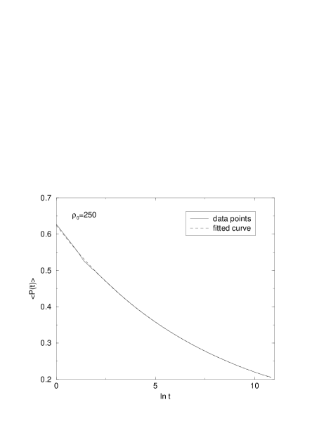
FIG. 5.: Same as Fig.2, but for $\rho_{0}=250$. The values of the fit parameters are $A=0.07\pm 0.02$, $B=0.55\pm 0.005$, $\theta_{nl}=0.13\pm 0.01.$

FIG. 6.: Same as Fig.3, but for $\rho_{0}=250$, with $\theta_{nl}=0.132.$

Notice that the values of $A$ obtained from the non-linear fits are quite small – $0.05(2)$ and $0.07(2)$ for $\rho_{0}=500$ and $\rho_{0}=250$ respectively. An equivalent fit for $\rho_{0}=50$ gives the larger value $A=0.17(2)$, so the data are consistent with the hypothesis that $A\to 0$ for $\rho_{0}\to\infty$, although the data are not good enough to extract the functional dependence of $A$ on $\rho_{0}$ in this limit.

FIG. 7.: Same as Fig.4, but for $\rho_{0}=250$. $\theta_{diff}=0.13\pm 0.01$.

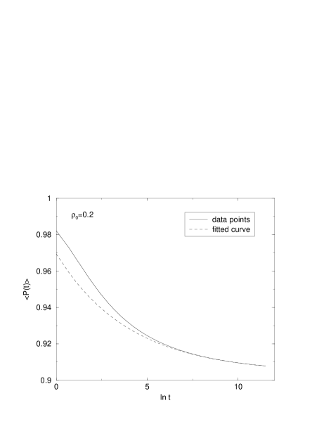
FIG. 8.: Same as Fig.2, but for $\rho_{0}=0.2$. The fit parameters are $A=0.90\pm 0.02$, $B=0.06\pm 0.005$, $\theta_{nl}=0.25\pm 0.01$.

Our low density results are presented below. We choose as our initial densities $\rho_{0}=0.2\textrm{ and }0.1$. In this regime, our simulations are performed on a lattice of size $10^{5}$ and run for $10^{5}$ time steps. The system takes longer to enter the asymptotic regime due to the low initial density and this is reflected in our extended number of time steps. We average our results over 50 runs. Figures 8 and 11 show the same type of non-linear fit, $\langle P(t)\rangle=A+B/t^{\theta_{nl}}$ that was used in Figures 2 and 5. The fit works well except at early times, and the fitted values are close to $\theta=1/4$ as anticipated. Note that the logarithmic scale for the abscissa greatly expands the early-time regime. The nonlinear fit was restricted to the range $10^{4}<t<10^{5}$ (i.e. the last 90% of each run), corresponding to $9.2<\ln t<11.5$. Figures 9 and 12 show the same data plotted as $\langle P(t)\rangle$ against $t^{-\theta_{nl}}$, and reveal the expected linear behaviour at late times. Finally, Figures 10 and 13 give the log-log plots for the differentiated data, from which the exponent estimates $\theta_{diff}$ are obtained. The slope is measured between the arrows in Figs. 10 and 13, corresponding to a similar region to that used for the non-linear fits.

FIG. 9.: Same as Fig.3, but for $\rho_{0}=0.2$. $\theta_{nl}=0.247$.

FIG. 10.: Same as Fig.4, but for $\rho_{0}=0.2$. Here the straight line has a gradient of -1/4. The gradient of the data, measured between the arrows, is $\theta_{diff}=0.25\pm 0.01$.

The estimates $\theta_{nl}$ and $\theta_{diff}$ of the persistence exponent, for both low and high density regimes, are summarised in Table 2. A natural consequence of the slow algebraic decay of the particle density is that the asymptotic regime, in the case $\rho_{0}\ll 1$, occurs only after many time steps. We expect the result $\theta\simeq 1/4$ for the low-density regime to manifest itself more clearly in systems run for a greater number of time steps.

FIG. 11.: Same as Fig.2, but for $\rho_{0}=0.1$. The fit parameters are $A=0.95\pm 0.02$, $B=0.05\pm 0.005$, $\theta_{nl}=0.26\pm 0.01$.

FIG. 12.: Same as Fig.3, but for $\rho_{0}=0.1$. $\theta_{nl}=0.264$.

$\rho_{0}$	$A$	$B$	$\theta_{nl}$	$\theta_{diff}$
500	$0.05\pm 0.02$	$0.57\pm 0.005$	$0.13\pm 0.01$	$0.12\pm 0.01$
250	$0.07\pm 0.02$	$0.55\pm 0.005$	$0.13\pm 0.01$	$0.13\pm 0.01$
0.2	$0.90\pm 0.02$	$0.06\pm 0.005$	$0.25\pm 0.01$	$0.25\pm 0.01$
0.1	$0.95\pm 0.02$	$0.05\pm 0.005$	$0.26\pm 0.01$	$0.27\pm 0.01$

TABLE 2. Values of the exponent $\theta$ in the relationship $P(t)=A+Bt^{-\theta}$, where $\theta$ has been evaluated according to a nonlinear curve fitting technique ($\theta_{nl}$) and through a method of numerical differentiation ($\theta_{diff}$). We expect, asymptotically, $\theta\simeq 0.1207$ for $\rho_{0}\gg 1$ and $\theta=1/4$ for $\rho_{0}\ll 1$.

FIG. 13.: Same as Fig.10 for $\rho_{0}=0.1$. $\theta_{diff}=0.27\pm 0.01$.

IV TYPE II PERSISTENCE

In this section we address the following question: What is the asymptotic probability $P(t)$ that a given site has never been visited by an $A$ or $B$ particle, in a one dimensional system of $A$ and $B$ random walkers subject to the $A+B\rightarrow\emptyset$ reaction-diffusion process? Necessarily, we pose this question within the context of a low initial density.

Our approach involves the introduction of a toy model, whose predictions we will compare to simulation results. The model consists of a system of noninteracting diffusing particles, with initial density $\rho_{0}=N(0)/L$, on a one-dimensional lattice with diffusion constant $D=1/2$. Note that the definition of $\rho_{0}$ in type II persistence refers to the total density of initial particles, in contrast to type I persistence, where $\rho_{0}$ referred to half the total density.

Particle decay is invoked by allowing each particle to vanish at every time step with some (usually time-dependent) probability. We define $f(t)$ to be the fraction of particles remaining at time $t$ i.e. $f(t)=\rho(t)/\rho_{0}$. We are then free to mimic the behaviour of any reaction-diffusion process by a suitable choice of $f(t)$.

The analysis of persistence in this toy model is straightforward. We first define the probability, $Q(x,t)$, that the origin has not been crossed by a given diffusing particle with initial position $x>0$. We define our lattice to be the interval $(-L/2,L/2)$. Then an elementary calculation gives $Q(x,t)=\textrm{erf}(x/2\sqrt{Dt})$, where we have assumed that $x\ll L$ and $L^{2}\gg Dt$, i.e. we have effectively taken the limit $L\to\infty$ in the calculation of $Q(x,t)$. A simple approach in the calculation of the number of persistent sites is to consider the first-passage-time distribution $P_{1}(t)$, where $P_{1}(t)dt$ is the probability that the first crossing of the origin occurs in $(t,t+dt)$. Then $P_{1}(t)dt=Q(x,t)-Q(x,t+dt)$ gives $P_{1}(t)=-dQ/dt$. Since the diffusing particle survives to time $t$ with probability $f(t)$, the probability for the origin to be persistent at time $t$ is given by,

$$Q(x,t) = 1-\int_{0}^{t}dt^{\prime}P_{1}(t^{\prime})f(t^{\prime})$$ (15)

$$= 1-\frac{x}{2\sqrt{D\pi}}\int_{0}^{t}\frac{ds}{s^{3/2}}f(s)\exp\left(-\frac{x^{2}}{4Ds}\right).$$ (16)

In the presence of many random walkers, whose random initial positions have a uniform distribution over space, the mean persistence is given by $\left<P(t)\right>=\left<Q(|x|,t)\right>^{\rho_{0}L}$ where $\rho_{0}L=N$ the total number of initial walkers and the average is over the initial position of a walker, assumed uniform in $(-L/2,L/2)$. This gives

$$\left<P(t)\right> = \left[1-\frac{1}{2L\sqrt{D\pi}}\int_{-\frac{L}{2}}^{\frac{L}{2}}dx|x|\int_{0}^{t}\frac{ds}{s^{3/2}}f(s)\right.$$ (18)

$$\left.\times\exp\left(-\frac{x^{2}}{4Ds}\right)\right]^{\rho_{0}L}.$$

For $L\rightarrow\infty$ we obtain,

$$\left<P(t)\right>=\exp\left(-2\rho_{0}\sqrt{\frac{D}{\pi}}\int_{0}^{t}\frac{ds}{s^{1/2}}f(s)\right).$$ (19)

A system of strictly diffusing particles with no decay is modelled by setting $f(s)=1$. In this case, $\left<P(t)\right>=\exp(-At^{1/2})$ where $A=4\rho_{0}\sqrt{D/\pi}$. In Fig. 14 we present a numerical verification of our calculation. The gradient of the graphs gives $-A$. The values of $A$ extracted from the data are compared with the numerical predictions in Table 3. The agreement is excellent.

FIG. 14.: Log-linear plot of the persistence for a system of noninteracting diffusing particles with no decay.

$\hskip 14.22636pt\rho_{0}\hskip 14.22636pt$	$A_{th}$	$A_{num}$
0.002	0.00319	$0.00320(5)$
0.005	0.00797	$0.00790(5)$

TABLE 3. The persistence properties of a system of noninteracting particles with zero probability of decay is described by $\left<P(t)\right>\sim\exp(-At^{1/2})$. Above we provide a comparison of the values of $A$ as deduced from the theory $A_{th}$ and from numerical simulations $A_{num}$.

Our model can also be applied to the $q$-state Potts model, which has $q$ distinct but equivalent ordered phases. The $A+A\rightarrow\emptyset$ model corresponds to $q=2$, while $A+A\rightarrow A$ corresponds to $q=\infty$. The density of walkers in the 1D Potts model is known to decay asymptotically according to [29],

$$\rho(t)\simeq\frac{q-1}{q}\frac{1}{\sqrt{2\pi Dt}}.$$ (20)

We can derive a generalised value of $\theta(q)$ for our toy model by substituting $f(s)=\rho(s)/\rho_{0}$ into Eq.(19) where $\rho(s)$ is given by Eq.(20). This gives,

$$\left<P(t)\right>\sim t^{-\theta_{T}(q)}\ ,$$ (21)

where

$$\theta_{T}(q)=\frac{\sqrt{2}}{\pi}\left(\frac{q-1}{q}\right)\ ,$$ (22)

and the subscript $T$ denotes ‘toy’. Despite the simplistic nature of our model, a power law decay for the persistence is predicted, in agreement with known results. Our expression for $\theta(q)$, (Eq.(22)) is clearly a poor approximation to the exact expression for the 1D Potts model obtained by Derrida et al [14].

$$\theta_{P}(q)=-\frac{1}{8}+\frac{2}{\pi^{2}}\,\left[\cos^{-1}\left(\frac{2-q}{\sqrt{2}\,q}\right)\right]^{2}\ ,$$ (23)

where the subscript $P$ denotes ‘Potts’. The values of the persistence exponent returned by our model for the $q=2$ and $q=\infty$ cases are, $\theta_{T}(q=2)=0.225$ and $\theta_{T}(q=\infty)=0.450$. The values given by Eq.(23) for the Potts model are $\theta_{P}(q=2)=3/8$ and $\theta_{P}(q=\infty)=1$. The encouraging feature of our toy model, however, is that the essential dynamics of the system leading to the power-law decay of the persistence in Eq.(21) is correctly identified as the $t^{-1/2}$ decay in the number of surviving random walkers at time $t$. If the number of surviving walkers decays as $t^{-\alpha}$ for large $t$, the toy model predicts, via Eq.(19), that the persistence will decay as a stretched exponential, $\langle P(t)\rangle\sim(-At^{1/2-\alpha})$, for $\alpha<1/2$, while $\langle P(t)\rangle$ will approach a non-zero constant for $\alpha>1/2$. The borderline case, $\alpha=1/2$, yields power-law decay of the persistence, as we have seen.

We naturally now turn our attention to the $A+B\rightarrow\emptyset$ reaction process to see if the correct time dependence of the persistence also emerges from our model. The density of $A$ and $B$ particles in this case in given by Eq. (13). Therefore $\left<\rho(t)\right>$ is given by,

$$\left<\rho(t)\right>\sim\frac{\rho_{0}^{1/2}}{(2\pi^{3})^{1/4}}(Dt)^{-1/4}\ ,\qquad\rho_{0}\ll 1\ ,$$ (24)

where $\rho(t)=\rho_{A}(t)+\rho_{B}(t)$ and $\rho_{0}=N(0)/L$. Substituting $f(s)=\rho(s)/\rho_{0}$ where $\rho(s)$ is given by Eq.(24) into Eq.(19) yields $\left<P(t)\right>\sim\exp(-Bt^{1/4})$ with $B=(2^{11}D/\pi^{5})^{1/4}\rho_{0}^{1/2}$. For the $A+B\rightarrow\emptyset$ reaction we therefore predict a stretched exponential decay of the persistence, with exponent $1/4$.

FIG. 15.: Log-linear plot of the persistence for the $A+B\rightarrow\emptyset$ reaction-diffusion process. $\left<P(t)\right>\sim\exp(-Bt^{\gamma})$ with $\gamma=1/4$.

The results of our numerical simulations are presented below. The simulations are performed on a one-dimensional lattice of size $10^{5}$ for $10^{5}$ time steps. We choose as our initial densities $\rho_{0}=0.02$ and $\rho_{0}=0.04$. A direct test of the stretched exponential prediction is obtained by plotting $\ln\langle P(t)\rangle$ against $t^{1/4}$, as in Figure 15. The fact that the data do not clearly show the expected straight line behaviour may indicate that the density is not yet in the regime where it is well described by the $t^{-1/4}$ form given by Eq.(24). Indeed, a direct study of the density indicates that the $t^{-1/4}$ behaviour is only evident at the latest times reached in the simulations. An alternative analysis involves differentiating the data with respect to $\ln t$ and presenting the result as a double logarithmic plot, as in Figures 16 and 17. Here there is evidence that the data approach the expected slope of $1/4$ at late times, though the noisy character of the differentiated data at the very latest times tends to obscure the asymptotic behaviour.

FIG. 16.: The log of the persistent fraction at time $t$ is numerically differentiated $(\Delta(\ln t)=0.1)$ and presented on a log-log plot for $\rho_{0}=0.02$ The gradient of the curve gives $\gamma$. The straight line has a slope of $1/4$.

FIG. 17.: Same as Fig.16 but for $\rho_{0}=0.04$.

In short, the data as presented in Figures 15, 16 and 17 are not clean enough to provide a convincing test of our prediction $\left<P(t)\right>\sim\exp(-Bt^{\gamma})$ with $\gamma=1/4$. The slow approach of the particle density to its asympotic $1/t^{1/4}$ behaviour is, in our view, the reason for this. A better test of our model, therefore, is to consider the persistence as a function of the actual running density of particles, rather than using the asymptotic behaviour of the density in Eq.(19). Taking the log of Eq.(19) and differentiating with respect to $\ln t$ yields,

$$-\frac{d\ln\left<P(t)\right>}{d\ln t}=2\sqrt{\frac{D}{\pi}}\rho(t)t^{1/2}\ ,$$ (25)

since $\rho_{0}f(t)=\rho(t)$, the running density. The left-hand side of Eq.(25) and $\rho(t)t^{1/2}$ (without the factor $2\sqrt{D/\pi}$) are plotted in Figures 18 and 19 for the two densities studied. The two curves agree rather well over the whole range of $\ln t$, except at the latest times, where the date are very noisy. The factor $2\sqrt{D/\pi}$ in Eq.(25), omitted from the plots, has the numerical value $\sqrt{2/\pi}\simeq 0.8$ (recall $D=1/2$), whereas Figures 18 and 19 suggest this number should be closer to unity. Given the crudeness of the toy model, however, the agreement between the data and the model is surprisingly good.

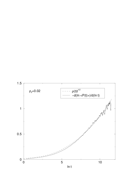
FIG. 18.: A direct test of Eq.(25) for $\rho_{0}=0.02$.

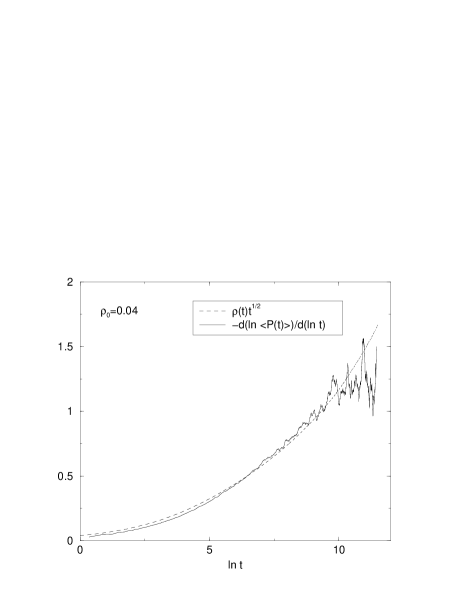
FIG. 19.: Same as Figure 18, but for $\rho_{0}=0.04$.

V SUMMARY

In this paper we have investigated the persistence properties of the $A+B\rightarrow\emptyset$ reaction-diffusion process using two distinct definitions of persistence. In type I persistence, we studied the fraction of sites which had never witnessed an annihilation process. In the high density limit $\rho_{0}\gg 1$ we argued that the persistence exponent is that which emerges from a study of the one dimensional diffusion equation, $\partial_{t}\phi=\partial_{xx}\phi$, where $\theta\simeq 0.1207$ [1], and presented data consistent with this result. In the low density limit $\rho_{0}\ll 1$ we argued that the persistence properties are governed by the same exponent that describes the decay of the particle density, giving $\theta=1/4$. Again, the data support this prediction. In type II persistence, we considered the probability that a site remained unvisited by either an $A$ or $B$ particle. Our approach, in this case, was to develop a toy model, which can be applied to any reaction-diffusion process and expresses the persistence properties in terms of the density of the reactants. For the $A+B\rightarrow\emptyset$ process the model predicts $\left<P(t)\right>\sim\exp(-Bt^{1/4})$. The data are consistent with this result when allowance is made for the actual time-dependence of the particle density (rather than just its asymptotic form). An obvious goal for future study would be to to place this stretched-exponential decay on a firmer theoretical foundation.

VI ACKNOWLEDGMENT

This work was supported by EPSRC (UK).

REFERENCES

- [1] S. N. Majumdar, C. Sire, A. J. Bray, and S. J. Cornell, Phys. Rev. Lett. 77, 2867 (1996).
- [2] For a recent review see S. Redner in Nonequilibruim Statistical Mechanics in One Dimension, ed. V. Privman, Cambridge University Press, 1997 and references therein.
- [3] R. Kroon, H .Fleurent, and R. Sprik, Phys. Rev. E 47, 2462 (1993).
- [4] J. T. MacDonald, J. H. Gibbs, and A. C. Pipkin, Biploymers 6, 1 (1968); G. M. Schütz, Int. J. Mod. Phys. B 11, 197 (1997).
- [5] J. M. J. Van Leeuwen and A. Kooiman, Physica A184, 79 (1992); M. Prähofer and H. Spohn, Physica A 233, 191 (1996).
- [6] J. Krug and H. Spohn, Solids Far From Equilibrium, ed. C. Godrèche, Cambridge University Press, 1991; T. Halpin-Healey and Y. -C. Zhang, Phys. Rep, 254, 215 (1995).
- [7] V. Kukla, J. Kornatowski, D. Demuth, I. Girnus, H. Pfeifer, L. Rees, S. Schunk, K. Unger, and J. Kärger, Science 272, 702 (1996); C. Rödenbeck, J. Kärger, and K. Hahn, Phys. Rev. E 55, 5697 (1997).
- [8] P. L. Krapivsky, E. Ben-Naim, and S. Redner, Phys. Rev. E 50 2474 (1994).
- [9] B. P. Lee, J. Phys A: Math. Gen. 27 2633 (1994).
- [10] B. P. Lee and J. Cardy, J. Stat. Phys. 80 971 (1995); J. Stat. Phys. 87 951 (1997).
- [11] M. Howard and J. Cardy, J. Phys. A: Math. Gen. 28 3599 (1995).
- [12] B. Derrida, A. J. Bray, and C. Godrèche, J. Phys. A 27, L357 (1994).
- [13] For a recent review see S. N. Majumdar, Curr. Sci. India 77, 370 (1999).
- [14] B. Derrida, V. Hakim, and V. Pasquier, Phys. Rev. Lett. 75, 751 (1995); J. Stat. Phys. 85, 763 (1996).
- [15] D. Stauffer, J. Phys. A 27, 5029 (1994).
- [16] B. Derrida, V. Hakim, and R. Zeitak, ibid. 77, 2871 (1996).
- [17] J. Krug, H. Kallabis, S. N. Majumdar, S. J. Cornell, A. J. Bray, and C. Sire, Phys. Rev. E 56, 2702 (1997).
- [18] A. J. Bray, B. Derrida, and C. Godrèche, Europhys. Lett. 27, 175 (1994); P. L. Krapivsky, E. Ben-Naim, and S. Redner, Phys. Rev. E 50, 2474 (1994); S. N. Majumdar and C. Sire, Phys. Rev. Lett. 77, 1420 (1996).
- [19] M. Marcos-Martin, D. Beysens, J. -P. Bouchaud, C. Godrèche, and I. Yekutieli, Physica D 214, 396 (1995).
- [20] W. Y. Tam, R. Zeitak, K. Y. Szeto, and J. Stavans, Phys. Rev. Lett. 78, 1588 (1997).
- [21] B. Yurke, A. N. Pargellis, S. N. Majumdar, and C. Sire, Phys. Rev. E 56, R40 (1997).
- [22] S. N. Majumdar, A. J. Bray, S. J. Cornell, and C. Sire, Phys. Rev. Lett. 77, 3704 (1996); K. Oerding, S. J. Cornell, and A. J. Bray, Phys. Rev. E 56, R25 (1997).
- [23] J. Cardy, J. Phys. A 28, L19 (1995); E. Ben-Naim, Phys. Rev. E 53, 1566 (1996); M. Howard, J. Phys. A: Math. Gen. 29, 3437 (1996); S. J. Cornell and A. J. Bray, Phys. Rev. E 54, 1153 (1996); G. Manoj and P. Ray, J. Phys. A: Math. Gen. 33 L109 (2000); A. J. Bray and S. J. O’Donoghue, Phys. Rev. E 62 3366 (2000).
- [24] D. Toussaint and F. Wilczek, J. Chem. Phys. 78 2642 (1983).
- [25] M. Bramson and J. L. Lebowitz, J. Stat. Phys. 62 297 (1991); J. Stat. Phys. 65 941 (1991).
- [26] K. Kang and S. Redner, Phys. Rev. Lett. 52 955 (1984).
- [27] S. Cornell, M. Droz, and B. Chopard, Physica A 188 322 (1992).
- [28] F. Leyvraz, J. Phys. A: Math. Gen. 25 3205 (1992).
- [29] T. Masser and D. ben-Avraham, Phys. Lett. A 275 382 (2000).