Granular flow down an inclined plane: Bagnold scaling and rheology

Abstract

We have performed a systematic, large-scale simulation study of granular media in two- and three-dimensions, investigating the rheology of cohesionless granular particles in inclined plane geometries, i.e., chute flows. We find that over a wide range of parameter space of interaction coefficients and inclination angles, a steady state flow regime exists in which the energy input from gravity balances that dissipated from friction and inelastic collisions. In this regime, the bulk packing fraction (away from the top free surface and the bottom plate boundary) remains constant as a function of depth $z$, of the pile. The velocity profile in the direction of flow $v_{x}(z)$ scales with height of the pile $H$, according to $v_{x}(z)\propto H^{\alpha}$, with $\alpha=1.52\pm 0.05$. However, the behavior of the normal stresses indicates that existing simple theories of granular flow do not capture all of the features evidenced in the simulations.

I Introduction

It is tempting to regard the behavior of granular materials as being a problem in engineering or applied science, inasmuch as the fundamental laws governing their constituent particles are well known. Being comprised of macroscopically large grains, granular materials obey classical mechanics, although the existence of friction and inelastic collisions complicates matters. However, while it is true that the collision of two grains is analytically tractable, an aggregate of such grains is a many-body system, whose macroscopic behavior cannot be simply related to the laws controlling individual constituents.

For this reason, a continuum treatment is often adopted, in which the variables are averaged properties whose governing equations are derivable, in principle, from the known microscopic laws. Among these averaged variables are the density $\rho$ and the stresses $\sigma_{\alpha\beta}$, which obey the Cauchy equations that enforce momentum conservation (or force balance if there are no accelerations). However, this set of equations is insufficient to solve for the stresses, since there are too few equations: in $D$ dimensions, there are $D(D+1)/2$ independent components of $\sigma_{\alpha\beta}$ (which is a symmetric tensor), but only $D$ equations of momentum conservation. Therefore, the Cauchy equations must be augmented by additional constitutive relations, possibly history-dependent, which tell how the material in question responds to the application of a force. It is in these constitutive relations that the specifics of the material in question come into play. In the case of steady state flow, which we will consider in this paper, constitutive equations would relate the strain-rate, $\dot{\gamma}_{\alpha\beta}$, to the stress.

In 1954, Bagnold [1] proposed that in inertial granular flow, the shear stress is proportional to the square of the strain-rate:

$$\sigma\propto\dot{\gamma}^{2}.$$ (1)

His argument, applied to the case of bulk granular flow, is predicated on a constant density profile. In practice, the presence of significant finite-size or wall effects often obscures Bagnold scaling. In this study, we report a set of numerical simulations of bulk granular flow down an inclined plane, so-called “chute flow”, in two and three dimensions. The geometry is simple: a layer of bulk granular material is placed on a flat plane of area $A$ (or line of length $L$ in 2D) on which grains have been glued, so as to form a rough base. The thickness of the layer is measured in terms of the pile height parameter $H\equiv Nd^{2}/A$ (or $Nd/L$ in 2D), where $N$ and $d$ are the total number of particles and their diameter, respectively. The plane is inclined at an angle $\theta$ and the flow is observed. The parameters controlling the flow are the macroscopic variables $\theta$ and $H$, as well as the microscopic variables determining the nature of interaction between two grains, such as grain friction $\mu$ and coefficient of restitution $\epsilon$.

In Ref. [2], we provided a summary of our simulations in two and three dimensions; in this paper we expand on these results both in depth and breadth for the case of steady state flow. The results obtained reveal the rich and surprising nature of the collective behavior of the system. For certain values of the parameters, we observe Bagnold scaling in stable steady state flow, with a constant density profile independent of depth. However, we also saw surprising examples of self-organization, including the flow-induced crystallization of a disordered state into one with much lower dissipation. In this regime (systems flowing on moderately smooth bottom surfaces), we found reentrant disordering as well, and even oscillations between ordered and disordered states. The effects of bottom surfaces are thoroughly discussed in a separate work [3]. In this paper, we concentrate on rough bottom surfaces for which the behavior is simpler.

These simulations also allow us to investigate more subtle aspects of chute flow, such as hysteresis in the angle of repose and normal stress inequalities not accounted for by any conventional continuum theory. Additionally, we were able to look for surface and bulk instabilities to flow at the angle of repose. In particular, we find that although the Bagnold rheology of flow near the angle of repose is a bulk rheology, the fundamental instability inducing the flow in three dimensions appears to be an instability of the surface layers of the granular medium.

Because granular materials are so common in nature, existing on many different length scales, there is a great amount of experimental data on a wide range of dynamic situations; shear flow and vibration experiments [4, 5, 6, 7], and studies of geological debris flows [8], to name just a few [9, 10]. There have been several moderately well-characterized experimental studies of granular flow down an inclined plane under laboratory conditions [11, 12, 13, 14, 15, 16]. Yet for all the intense activity in this field over the years, the rheology of granular systems still remains a largely unsolved problem.

There has been some work on continuum modeling of chute flow; for a review of continuum based ideas see Savage [17] and references therein. Other theoretical analyses (sometimes combined with case-specific simulation verification), specifically applied to chute flow geometries, attempt to calculate density and velocity profiles [18, 19, 20, 21], but a general consensus on the qualitative features of these profiles has yet to be reached.

The state of the art of computer simulations of chute flow is much less satisfactory because of the enormous equilibration times needed to set up steady flow. In three dimensions, simulations have been performed for rather thin piles, which provides insight into only a small region of phase space [16, 22, 23]. Simulations of two-dimensional flows also report on small systems, and it is unclear whether these studies are carried out in the steady state regime or whether the data reported are transient [24, 25, 26, 27]. The basics behind granular simulations are available in Refs. [28] for 2D and [23] for 3D.

Our simulations attempt a systematic 3D study of chute flows. Unfortunately, we probe regions of phase space difficult to access in experiment. In a typical 3D experiment the flow is induced through a hopper-feeder mechanism which controls the flow rate of the system, but not the thickness of the flowing sample, which is chosen spontaneously by the system. Thus, much experimental data is for flowing piles 10-15 particles high, whereas most of our simulations focus on moderate to thick piles, greater than 30 particles. Simulation results for systems smaller than 10 - 15 particles high do not show the same scaling as that for thicker systems [11]. Also, 3D experiments are usually carried out in narrow channels of order 10 particles wide or less, where side-wall effects may have a significant role in the observed behavior. Our simulations are periodic in this, the vorticity, direction, and we have yet to study wall effects. We suspect that most discrepancies that may exist between different experimental and simulation studies are due to such differences in the detailed nature of the systems studied.

Because of the complexity of flowing granular systems, it is useful to first define the region of study. In order to determine the phase boundaries of fully developed, steady state flow, we have performed a series of simulations of inclined plane gravity driven flows in two and three dimensions in an attempt to define the region of phase space for which steady state flows exist. A typical configuration snapshot in 3D, defining the computational geometry, is shown in Fig. 1.

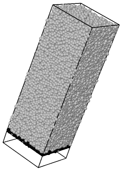
FIG. 1.: Typical 3D snapshot for chute flow: N=24,000, with bottom surface dimensions 20x20 diameters shown by the black particles fixed to the bottom plate; tilt angle $\theta=24^{o}$, coefficient of restitution $\epsilon=0.88$, and friction coefficient $\mu=0.50$. Flow is directed down the incline.

In our simulations, initiation of flow is achieved by tilting at a large angle ($24-30^{o}$) to induce flow. This procedure removes any configuration construction history effects. We then reduce the inclination to a lower angle and allow the simulation to run until we observe a steady state flow regime (if one exists). We define steady state as flow wherein the energy input from gravity balances that dissipated from friction and collisions; so that the total kinetic energy of the system reaches a macroscopically constant value. In this case, the results are independent of sample history.

In Fig. 2, we draw phase boundaries for both two and three dimensional flows as a function of the external control parameters: tilt angle $\theta$ and pile height $H$. This should be compared to a similar experimental determination recently obtained by Pouliquen [29]. The salient features are the existence in both 2D and 3D of three principal regions, corresponding to no flow, stable flow, and unstable flow. For a system of given thickness and fixed microscopic interaction parameters, these three regions are separated by two angles: $\theta_{r}$, the angle of repose, and $\theta_{max}$, the maximum stability angle, the largest angle for which stable flow is obtained, shown by a solid and dashed lines in Fig. 2, respectively.

(a) (b)

FIG. 2.: Phase behavior of granular particles in chute flow geometry, characterized by pile height $H$ vs. tilt angle $\theta$ for monodisperse systems in (a) 2D with $\mu=0.50$ and $\epsilon=0.92$ (identified as Model L2 in Table I), and (b) 3D with $\mu=0.50$ and $\epsilon=0.88$ (identified as Model L3). Both figures are for the spring dash-pot interaction model with rough bottom surface. Solid circles indicate region of steady state flow, open symbols correspond to no flow or unstable flow. In 3D we have identified hysteretic flow as x.

For $\theta<\theta_{r}$, granular flow cannot be sustained. In the region $\theta_{r}<\theta<\theta_{max}$, we obtain steady state flow with packing fraction independent of depth. The region of constant packing fraction in the flowing material for steady state systems is accompanied by a smoothly varying, non-linear velocity profile. For $\theta>\theta_{max}$, the development of a shear thinning layer at the bottom of the pile results in lift-off and unstable acceleration of the entire pile. The exact locations of these phase boundaries depend on the model parameters such as $\mu$ and $\epsilon$. For instance, in 2D, if $\epsilon$ is reduced from $0.92$ to $0.82$, the maximum angle of steady-state flow increases from $\approx 23^{o}$ to $26^{o}$. Similarly, reducing $\mu$ typically reduces the range of stable flow.

It is well known that granular systems exhibit hysteresis. Such behavior is usually attributed to system preparation and associated history effects [30]. Although we observe three distinct regimes, the behavior close to the phase boundaries is sensitive to the procedure for the initiation of flow. Indeed, we have observed hysteresis in our 3D simulations when approaching $\theta_{r}$ from either side, particularly for thinner piles. The hysteresis was significantly reduced upon increasing pile height $H$. Crystallization of the 2D monodisperse pile upon the arrest of flow was primarily responsible for the large hysteresis observed in that case.

Besides the phase diagram, our most important results concern the detailed structure and rheology of the steady-state flowing regime. In this regime, we do see a constant density profile with height, as well as the Bagnold scaling of Eq.(1). The amplitude of the strain rate goes to zero at the angle of repose; thus relations such as Eq.(1) possess an additional strong angular dependence.

We also analyzed the normal stresses in the flowing state, and found a number of results, most notably that the normal stress perpendicular to the free surface, $\sigma_{zz}$, is approximately, but not exactly, equal to the normal stress parallel to the flow, $\sigma_{xx}$.

There are two fundamental puzzles in these results for the rheology of chute flow. The first, and smaller, puzzle is the appearance of an anomalous normal stress difference $\sigma_{zz}-\sigma_{xx}$. We have been unable to define a simple, local, dimensionally consistent and rotationally invariant constitutive relation connecting $\sigma$ to $\dot{\gamma}^{2}$ that recovers this behavior.

The second, and deeper puzzle, is the relationship between the rheology and the Coulomb yield criterion. As the angle of repose is approached from above, the amplitude of the flow goes to zero, but the tensor structure of $\sigma$ remains approximately liquid-like, instead of recovering the large normal stress difference characteristic of the Coulomb yield criterion, which presumably applies to the static pile at the angle of repose. The one exception to this observation is the surface stress in three dimensions, where the normal stress differences do become large as the angle of repose is approached, suggesting that surface yield may control the failure of the static state.

In the bulk, however, we are left with a transition to a static state that appears continuous in shear rate, but is apparently discontinuous in normal stress. We do not believe that an understanding of chute flow rheology is possible without resolving this seeming paradox.

We present the simulation scheme in Section II, detailing the inter-particle force laws. In Section III, we report our comprehensive simulation analysis, including the behavior of the density and velocity profiles for our systems with varying interaction parameters. In Section IV, we present a detailed discussion of stress analysis and rheology of chute flow systems. In Section V we summarize our findings.

II Simulation Methodology

We use the methods of molecular dynamics to perform 2D and 3D simulations of granular particles. For this study we model $N$ mono-disperse spheres of diameter $d$ and mass $m$, supported on the $xy$-plane by a rough bed. The computational geometry of the present 3D system consists of a rectangular box with periodic boundary conditions in the $x$ (flow)- and $y$ (vorticity)-directions and constrained in the vertical $z$-direction by a fixed rough, bottom wall and a free top surface, as in Fig. 1. Simulations in periodic cells attempt to study flow down infinitely long and wide chutes, while using a finite number of particles.

In 3D, the fixed bottom is constructed from a random conformation of spheres of the same diameter $d$ as those in the bulk by taking a slice with areal fraction very close to random close packing (approximately 1.2 particle diameters thick), from a previously packed state. This simulates an experimental procedure whereby glue is spread over the original smooth chute surface and particles are then sprinkled onto this surface to construct a rough floor approximately one particle layer thick. For 2D studies, the bottom wall is constructed from a regular array of spheres of diameter $2d$ and particle motion is restricted to the $xz$-plane.

We employed a contact force model that captures the major features of granular interactions. In 2D, interactions between (projected) spheres are modeled using a linear spring model with velocity-dependent damping (the spring-dashpot interaction) and static friction. In 3D the spring-dashpot model and static friction are also used, as well as Hertzian contact forces with static friction. In the presentation of the results, we will specify which model is employed, and discuss the differences.

The implementation of the contact forces, both the normal forces and the shear (friction) tangential forces, is essentially a reduced version of that employed by Walton and Braun [22], developed earlier by Cundall and Strack [28]. More recent versions of these models now exist [31, 32, 33]. We ignore hysteretic effects between loading or unloading normal contacts and we do not differentiate between frictional directions at the same contact point at different time-steps as does Walton[23].

Static friction is implemented by keeping track of the elastic shear displacement throughout the lifetime of a contact. For two contacting particles $\{i,j\}$, at positions $\{{\bf r}_{i},{\bf r}_{j}\}$, with velocities $\{{\bf v}_{i},{\bf v}_{j}\}$ and angular velocities $\{{\mathbf{\omega}}_{i},{\mathbf{\omega}}_{j}\}$, the force on particle $i$ is computed as follows: the normal compression $\delta_{ij}$, relative normal velocity ${\bf v}_{n_{ij}}$, relative tangential velocity ${\bf v}_{t_{ij}}$ are given by

$$\delta_{ij} = d-r_{ij},$$ (2)

$${\bf v}_{n_{ij}} = ({\bf v}_{ij}\cdot{\bf n}_{ij}){\bf n}_{ij},$$ (3)

$${\bf v}_{t_{ij}} = {\bf v}_{ij}-{\bf v}_{n_{ij}}-\frac{1}{2}({\mathbf{\omega}}_{i}+{\mathbf{\omega}}_{j})\wedge{\bf r}_{ij},$$ (4)

where ${\bf r}_{ij}={\bf r}_{i}-{\bf r}_{j}$, ${\bf n}_{ij}={\bf r}_{ij}/r_{ij}$, with $r_{ij}=|{\bf r}_{ij}|$, and ${\bf v}_{ij}={\bf v}_{i}-{\bf v}_{j}$. The rate of change of the elastic tangential displacement ${\bf u}_{t_{ij}}$, set to zero at the initiation of a contact, is given by

$$\frac{d{\bf u}_{t_{ij}}}{dt}={\bf v}_{t_{ij}}-\frac{({\bf u}_{t_{ij}}.{\bf v}_{ij}){\bf r}_{ij}}{r_{ij}^{2}}.$$ (5)

The second term in Eq.(5) arises from the rigid body rotation around the contact point and insures that ${\bf u}_{t_{ij}}$ always lies in the local tangent plane of contact. Normal and tangential forces acting on particle $i$ are given by

$${\bf F}_{n_{ij}} = f(\delta_{ij}/d)(k_{n}\delta_{ij}{\bf n}_{ij}-\gamma_{n}m_{\rm eff}{\bf v}_{n_{ij}}),$$ (6)

$${\bf F}_{t_{ij}} = f(\delta/d)(-k_{t}{\bf u}_{t_{ij}}-\gamma_{t}m_{\rm eff}{\bf v}_{t_{ij}}),$$ (7)

where $k_{n,t}$ and $\gamma_{n,t}$ are elastic and viscoelastic constants respectively, and $m_{\rm eff}=m_{i}m_{j}/(m_{i}+m_{j})$ is the effective mass of spheres with masses $m_{i}$ and $m_{j}$. The corresponding contact force on particle $j$ is simply given by Newton’s third law, i.e., ${\bf F}_{ji}=-{\bf F}_{ij}$. For spheres of equal mass $m$, as is the case here, $m_{\rm eff}=m/2$; $f(x)=1$ for the linear spring-dashpot model, denoted henceforth as Model L, or $f(x)=\sqrt{x}$ for Hertzian contacts with viscoelastic damping between spheres, denoted as Model H.

Our results are given in non-dimensional quantities by defining the following normalization parameters: distances, times, velocities, forces, elastic constants, and stresses are respectively measured in units of $d,~{}t_{o}=\sqrt{d/g},~{}v_{o}=\sqrt{gd},~{}F_{o}=mg,~{}k_{o}=mg/d,~{}\text{ and }~{}\sigma_{o}=mg/d^{2}$. For a realistic simulation of glass spheres with diameter $d=100\mu m$, the appropriate elastic constant $k^{glass}_{n}=O(10^{10})$ necessitates a very small time-step for accurate simulation, prohibiting any large-scale study. In our simulations, we typically use a value for $k_{n}=O(10^{5})$ which we believe captures the general behavior of intermediate-to-high-$k$ systems, thus offering a reasonable representation of realistic granular materials (we discuss this aspect further in Section III B). A complete list of model parameters used in our standard simulation set, which consists of 2D and 3D versions of Model L (L2 and L3), and a 3D version of Model H (H3), are given in Table I.

In a gravitational field g, the translational and rotational accelerations of particles are determined by Newton’s second law, in terms of the total forces and torques on each particle $i$:

$${\bf F}_{i}^{\rm tot} = m_{i}{\bf g}+\sum_{j}{{\bf F}_{n_{ij}}+{\bf F}_{t_{ij}}};$$ (8)

$$\mbox{\boldmath{$\tau$}}_{i}^{\rm tot} = -\frac{1}{2}\sum_{j}{{\bf r}_{ij}\wedge{\bf F}_{t_{ij}}}.$$ (9)

The amount of energy lost in collisions is characterized by the inelasticity through the value of the coefficient of restitution. For Model L, there are separate coefficients, $\epsilon_{n}$ and $\epsilon_{t}$, for the normal and tangential directions which are related to their respective damping coefficients $\gamma_{n,t}$ and spring constants $k_{n,t}$:

$$\epsilon_{n,t}=\exp(-\gamma_{n,t}t_{col}),$$ (10)

where the collision time $t_{col}$ is given by,

$$t_{col}=\pi\left(2k_{n}/m-\gamma_{n}^{2}/4\right)^{-1/2}.$$ (11)

The value of the spring constant should be large enough to avoid grain interpenetration, yet not so large as to require an unreasonably small simulation time step $\delta t$, since an accurate simulation typically requires $\delta t\sim t_{col}/50$. For Model H, the effective coefficients of restitution depend on the initial velocity of the particles.

The static yield criterion, characterized by a local particle friction coefficient $\mu$ [34], is modeled by truncating the magnitude of ${\bf u}_{t_{ij}}$ as necessary to satisfy $|{\bf F}_{t_{ij}}|<|\mu{\bf F}_{n_{ij}}|$. Thus the contact surfaces are treated as “stuck” while $F_{t_{ij}}<\mu F_{n_{ij}}$, and as “slipping” while the yield criterion is satisfied. This “proportional loading” approximation [35] is a simplification of the much more complicated and hysteretic behavior of real contacts [36]. To test the robustness of the proportional loading assumption, we also carried out simulations with Model L in which ${\bf u}_{t}$ is not truncated but the local yield criterion $F_{t}<\mu F_{n}$, is implemented. Note that we do not believe this to be a physically reasonable choice. Results for the two cases are similar, although the average kinetic energy is somewhat smaller (by approximately $18\%$ for Model L2) when $u_{t}$ is truncated compared to those simulations when $u_{t}$ is unbounded.

The components of the stress tensor $\sigma_{\alpha\beta}$ within a given sampling volume $V$ are computed as the sum over all particles $i$ within that sampling volume of the contact stress (virial) and kinetic terms,

$$\sigma_{\alpha\beta}=\frac{1}{V}\sum_{i}\left[\sum_{j\neq i}\frac{{r}_{ij}^{\alpha}F_{ij}^{\beta}}{2}+m_{i}(v_{i}^{\alpha}-\overline{v^{\alpha}})(v_{i}^{\beta}-\overline{v^{\beta}})\right],$$ (12)

where $F_{ij}^{\beta}=F_{n_{ij}}^{\beta}+F_{t_{ij}}^{\beta}$, and $\overline{\bf v}$ is the time-averaged velocity of the particles within the sampling volume $V$. The time-averaged velocity must be subtracted since the kinetic portion of the stress tensor is entirely due to fluctuations in the velocity field.

For Hertzian contacts [37], the ratio $k_{t}/k_{n}$ depends on the Poisson ratio of the material, and is about 2/3 for most materials. For ease in our simulations, we use a value $k_{t}/k_{n}$=2/7, which makes the period of normal and shear contact oscillations equal to each other for Model L [38]. However, the contact dynamics are not very sensitive to the precise value of this ratio. We have performed simulations with different values of $k_{t}/k_{n}$ to test how this ratio may affect our results; different values of this ratio yield nearly identical results. The only difference we observe is a slight increase in the total, averaged kinetic energy (KE) of the system when $k_{t}/k_{n}>2/7$, and a decrease for $k_{t}/k_{n}<2/7$. For example, when we set $k_{t}/k_{n}=2/3$ instead of $2/7$, the total averaged KE increases by about $10\%$, whereas all other macroscopic quantities measured in the simulations, such as density and stress, remain essentially unchanged.

Similarly, although all results reported here are for $\gamma_{t}/\gamma_{n}=0$ (i.e. no rotational velocity damping term) we have also carried out simulations to measure the effect of introducing rotational damping, $\gamma_{t}/\gamma_{n}>0$. When we set $\gamma_{t}=\gamma_{n}$, we observe a slight decrease, of about $8\%$, in the total averaged KE, compared with those simulations that have $\gamma_{t}=0$. Making $\gamma_{t}/\gamma_{n}$ non-zero quickens the approach to the steady state by draining out more energy. However, all other quantities are, again, unchanged. We discuss reasons why we observe minimal changes with these interaction parameters in Sec. III B.

Typical values for the friction coefficient $\mu$ range between, 0.4 and 0.6 for many materials. We chose $\mu=0.50$ for most of our simulations, though variations in $\mu$ will be discussed in Sec. III B. Similarly, the value of $\epsilon$ is chosen to reflect the properties of a realistic granular particle.

Model	$D$	$f(x)$	$k_{n}$	$\gamma_{n}$	$k_{t}/k_{n}$	$\gamma_{t}/\gamma_{n}$	$\mu$	$\epsilon$
L2	2	1	$2\cdot 10^{5}$	$33.5$	2/7	0	0.50	0.92
L3	3	1	$2\cdot 10^{5}$	$50.0$	2/7	0	0.50	0.88
H3	3	$\sqrt{x}$	$2\cdot 10^{5}$	$50.0$	2/7	0	0.50	-

TABLE I.: Parameter values used in our standard simulation set for the 2D and 3D linear spring models (Models L2 and L3, $f(x)=1$), and the 3D Hertzian model (Model H3, $f(x)=\sqrt{x}$). For Model H3, $\epsilon$ is velocity dependent.

The equations of motion for the translational and rotational degrees of freedom are integrated with either a third-order Gear predictor-corrector or velocity-Verlet scheme [39] with a time-step $\delta t=10^{-4}$ for $k_{n}=2\times 10^{5}$. All data was taken after the system had reached the steady state. To reach the steady state, simulations were required to run for $~{}1-2\times 10^{7}\delta t$ when starting from a non-flowing state for $N<10,000$, and the largest system in 2D $(H=200)$ required a run time of $~{}2-5\times 10^{8}\delta t$. On a 500 MHz DEC Alpha processor, our code requires about 5 days to simulate 10 million timesteps of a 3D 8000-particle granular system. We have also created a parallel version of the 3D code using the standardized MPI message-passing library. The parallel code partitions the simulation domain into small 3D sub-blocks using the methods described in [40]. Even on a cluster computer with relatively low interprocessor communication bandwidth, the code runs at high parallel efficiencies so long as we simulate 1000 or so particles per processor. For example, on 8 processors of our Alpha/Myrinet cluster, we can simulate 15 million timesteps/day of the same 8000-particle system.

For the imposition of chute flows with varying tilt angles, we rotate the gravity vector ${\bf g}$ in the $xz$-plane by the tilt angle $\theta$ away from the $-{\bf z}$ direction — flow is from left to right in this sense. This means that the ${\bf z}$-axis is always normal to the free surface. In 3D the area of the bottom is $A=L_{x}L_{y}$ where $L_{x}$ and $L_{y}$ are the dimensions of the simulation cell in the $x$ and $y$ directions respectively. For the 3D simulations, we define a measure of the height of the pile by defining $H\equiv Nd^{2}/A$ as the pile height if it were sitting on a level plane at rest in a simple cubic lattice. For example, for $N=8000$ and $L_{x}=20d$ and $L_{y}=10d$, $H=40$ (although due to the precise configuration, the actual measured height $\approx 37$). This is a useful definition for comparing between different system sizes. We study a range of system sizes, $1000\leq N\leq 20000$. For the largest system, $H=100$. The influence of other wall dimensions $L_{x},~{}L_{y}$ was also studied. For the 2D runs, the $x$-dimension of the periodic side is fixed at $100d$ (i.e. $50$ large particles long) and the pile height $2\leq H\leq 200$, i.e. $N=200-20000$.

In 2D, the initial state was constructed by building a triangular lattice of particles. The tilt angle was then increased until flow occurred. The initial flow occurred only for $\theta\gtrsim 23^{o}$. This minimum value to induce flow depends on the size and spacing of bottom plate particles. The initial failure occurred mostly at the bottom of the pile, followed by movement of a dilation front toward the top of the pile as shown in Fig. 3. Once this initial steady state was achieved, the angle $\theta$ was adjusted to its desired value, and the system equilibrated to its final steady state. In 3D, we started the system from a randomly diluted simple cubic lattice. The angle was then increased to a large angle $\theta=30^{o}$ to induce disorder and settling of particles. The angle $\theta$ was then decreased to the desired value and flow allowed to continue until a steady state was reached, before measurements were taken.

In 3D, to test for hysteresis near $\theta_{r}$, $\theta$ was reduced to below $\theta_{r}$ until the system settled down into a disordered state and stopped flowing. $\theta$ was subsequently increased to $\theta_{r}^{flow}$ and the system began flowing. This angle of flow initiation was sometimes different from the angle of cessation of flow $\theta_{r}^{stop}$ when taking a flowing state and then lowering $\theta$ down to $\theta_{r}^{stop}$ to stop the flow. However, this small hysteretic behavior, in 3D, only occurs for thin piles at low angles.

In 2D the equivalent phase diagram can only be constructed by taking a flowing state at angle $\theta$ and then lowering to $\theta_{r}^{stop}$. Once the 2D state stops flowing the system spontaneously crystallizes into a polycrystalline ordered state. To induce flow from this ordered state requires increasing $\theta$ to a much higher angle than $\theta_{r}^{stop}$.

III Results: Velocity and Density Profiles

A Kinematics of steady state systems

We focus our main attention on the regime of steady state flow for moderate to deep piles, for which $\theta_{r}$ is independent of depth. In Fig. 4 we plot the density and velocity (in the direction of flow) $z$-profiles over a range of inclination angles $\theta$, for a series of simulations in 2D and 3D. Figure 4(a) is for a 2D system (Model L2, cf. Table I) of N=10,000 particles, corresponding to $H=100$. In Fig. 4(b), the equivalent 3D model (Model L3 with $N=8,000,H=40$), denoted by the open symbols, is compared to the 3D Hertzian model (Model H3). The tilt angle was varied between $18^{o}-30^{o}$ in all cases. In 2D the system becomes unstable to an accelerating flow above $23^{o}$ and in 3D the unstable flow regime is observed above $26^{o}$.

In both 2D and 3D, the packing fraction remains constant over almost 40 layers in 3D, and 100 layers in 2D. For all steady state systems, as the tilt angle is increased, the value of the bulk packing fraction decreases. This decrease accompanies a growing dilated region (of lower packing fraction) near the free surface at the top. All the velocity profiles are concave, and velocities increase in value with increasing tilt angles. Consequently, the total kinetic energy of the system rises with increasing angle [41].

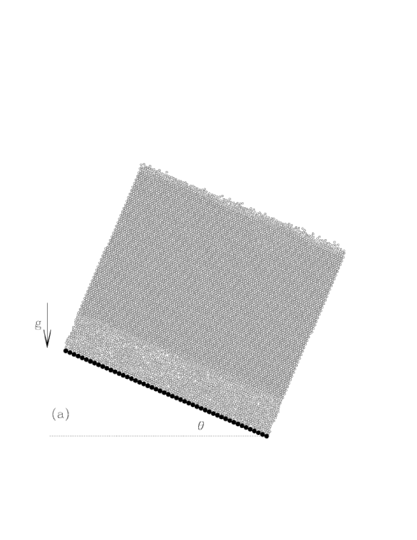
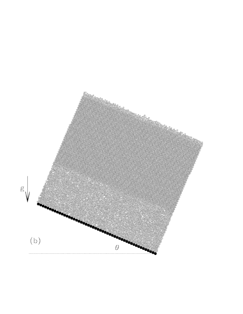
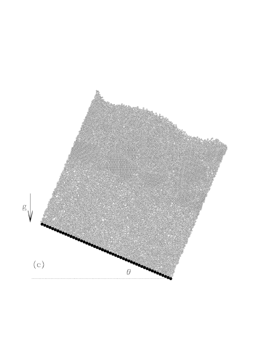
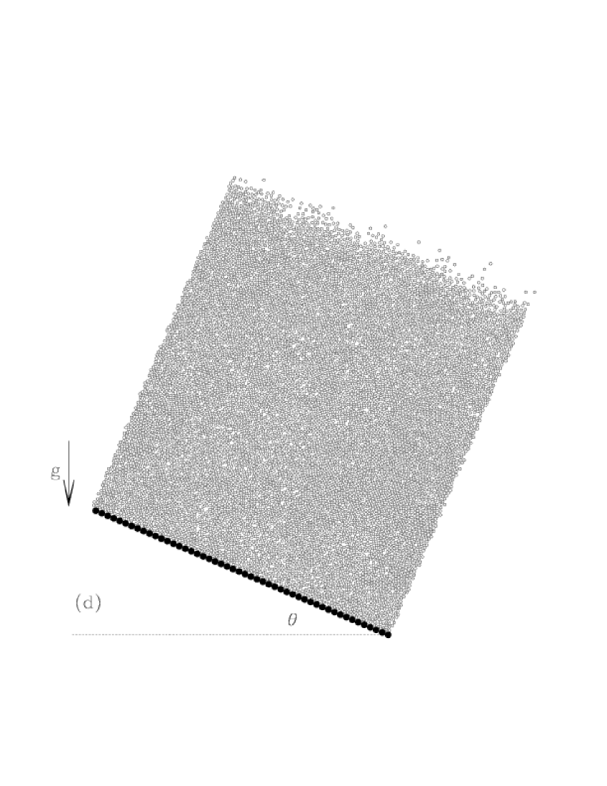
FIG. 3.: Time sequence of a typical configuration in 2D following an instantaneous change in the inclination angle $\theta$ from $0^{o}$ to $24^{o}$. Results are for $N=10000,~{}\mu=0.50$, and $\epsilon=0.82$, and for times $t$ = a) 100, b) 400, c) 600, d) 6000. Flow is left to right. As the flow progresses, the dilational front propagates upwards through the system, destroying the initial ordered array; the pile consequently “fluffs” up.

(a) (b)

FIG. 4.: Packing fraction $\phi$ and velocity $v_{x}$ profiles, as a function of distance from bottom $z$, for (a) 2D spring–dash-pot model (Model L2), with $H=100$, at tilt angles of $\theta$=18, 19, 20, 21, 22, 23 degrees. (b) 3D, $H=40$ systems at $\theta$=20, 22, 24, 26 degrees, with Model L3 (open symbols) and Model H3 (solid lines).

We monitor vertical mixing of the bulk by measuring the bulk-averaged, mean-square displacement of particles over time. Figure 5 shows the mean-square displacement of particles normal to the surface $<z^{2}>$ as a function of simulation time for Model L3, over a range of tilt angles. The linear relationship demonstrates well-defined diffusive motion in the z-direction, suggesting thorough mixing in the system. Similar results are observed in 2D. At long times $<z^{2}>$ will reach a constant due to the finite height of the pile.

FIG. 5.: z-component of the mean square displacement for 3 angles, $\theta=21^{o},22^{o}$, and $23^{o}$, for Model L3, with $H=40$.

By observing a sequence of snapshots (not shown here) of tracer particles at various heights in the bulk, we also find that diffusion is somewhat faster nearer the bottom of the pile. This is indicative of the fact that fluctuations in the particle velocities are greater closer to the bottom wall. Fig. 6 depicts the diagonal components of the kinetic part of the stress tensor, $\rho<(\delta v^{\alpha})^{2}>$, where $\rho$ is the mass density and $\delta v^{\alpha}=v^{\alpha}-\overline{v^{\alpha}}$, at three different angles for Model L3. Indeed we do find that the velocity fluctuations (frequently termed “granular temperature” in the literature of dilute granular flows) are greatest at the bottom of the pile (away from the actual plate) and decrease with height until the values appear to level off at the top free surface.

FIG. 6.: Profiles of the kinetic portion of the diagonal elements of the stress tensor $\rho<(\delta v^{\alpha})^{2}>$, normalized by their maximum value along the curve, for Model L3 inclined at $21^{o}~{}(---)$, $23^{o}~{}($—$)$, and $25^{o}~{}(-\cdot)$.

This behavior partially illustrates how the pile is able to maintain a constant density profile, even though the stresses increase towards the bottom, and the flowing pile has a finite compressibility, as evidenced by the changing density as a function of tilt angle $\theta$. Particles deeper into the pile experience increasing compaction forces due to the load of the particles above, yet a constant density is maintained through the increased particle velocity fluctuations.

The data sets shown in Fig. 4 are for one system size only. In Fig. 7 density and velocity profiles for systems of varying heights are compared. The densities measured deep in the pile, as well as the density and strain rate profiles near the surface, are independent of the overall height of the pile. This suggests that the rheology of the system is local in this regime; i. e., that constitutive relations locally relate stress and strain rate. For reasons alluded to in Sec. IV D, we have been unable to identify these constitutive relations.

(a) (b)

FIG. 7.: Density and velocity profiles for (a) 2D systems (Model L2) for $\theta=20^{o}$ with sizes $H=200,~{}100,~{}50,~{}25$ and (b) 3D systems (Model L3) for $\theta=24^{o}$ with sizes $H=100,~{}60,~{}50,~{}60$ .

FIG. 8.: Density and velocity profiles for thin systems (Model L2), with $H=10$, at $20^{o}$ and $23^{o}$. These profiles are very different from the thicker piles.

We note that the behavior observed in Figs. 4 and 7 is true only for $H\gtrsim 20$. For smaller piles, such as those commonly studied experimentally [13], the behavior is very different, as seen in Fig. 8, where a linear velocity profile is evident. Recent experimental studies of thin piles in inclined plane geometries also report linear velocity profiles [11].

B Dependence on Interaction Parameters

In this subsection, we investigate the sensitivity of these results to the particle interaction parameters. We independently vary the internal coefficient of friction $\mu$, the coefficient of restitution $\epsilon$, and the value of the spring constant $k_{n}$. We observe that while the density of the bulk material does not depend sensitively on these interaction parameters, the velocity profiles do.

Figure 9 shows the sensitivity to the friction coefficient $\mu$ by depicting density, velocity, and strain rate profiles for: (a) Model L2 with $H=50$ and $\theta=20^{o}$, where $\mu=0.15,~{}0.25,~{}0.50,~{}1.0$, and (b) Model L3 with $H=40$ and $\theta=22^{o}$, for values of $\mu=0.15,~{}0.25,~{}0.5,~{}1.0$. The data suggest that there is minimal change in the bulk density over this range in $\mu$. In the bottom panels of Fig. 9, the shear rate $\frac{\partial v_{x}}{\partial z}$ scaled by $\frac{\partial v_{x}^{max}}{\partial z}$ is plotted for the various values of $\mu$.

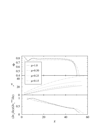
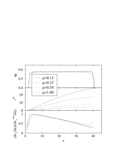
(a) (b)

FIG. 9.: Density, velocity, and strain rate profiles for different values of the particle friction coefficient for: (a) Model L2 at $\theta=20^{o},H=50$ for $\mu=0.15,~{}0.25,~{}0.50,~{}1.0$, and (b) Model L3 at $\theta=22^{o},H=40$ for $\mu=0.15,~{}0.25,~{}0.50,~{}1.0$.

Similarly, Fig. 10 shows the profiles for the same systems as described in Fig. 9, but with a fixed $\mu=0.5$ and varying coefficients of restitution $\epsilon$, i.e., varying the inelasticity of the system. Again we see that variations in $\epsilon$ have little effect on the flow behavior of these systems, particularly in 3D, provided that the system is able to reach steady state. [For low $\mu$ ($\approx 0.10$) and high $\epsilon$ ($\approx$ 0.96 for 2d and 0.98 for 3d), the systems become unstable.]

(a) (b)

FIG. 10.: Density and velocity profiles for different values of $\epsilon$ for (a) Model L2 at $\theta=20^{o},H=50$ for $\epsilon=0.72,0.82,0.92,0.96$, and (b) Model L3 at $\theta=22^{o},H=40$ for $\epsilon=0.58,0.78,0.88,0.98$.

Another microscopic parameter we have investigated is the effective hardness of the particle, determined by the value of the spring constant $k_{n}$. We vary $k_{n}$ and keep $\epsilon$ constant by adjusting the value of $\gamma_{n}$. Simulations investigating this parameter can be time-consuming: increasing $k_{n}$ by a factor of 100 requires a reduction in the time-step by a factor of 10. Fortunately, as Fig. 11, (measured for Model L2 with $\theta=20^{o},H=50$) indicates, the effect of variations in $k_{n}$ is minimal, provided $k_{n}$ is sufficiently large.

FIG. 11.: Density and velocity profiles for different values of the spring constant $k_{n}$, for Model L2 at $\theta=20^{o},H=50$.

FIG. 12.: Tilt dependence of the packing fraction in the region of constant packing fraction, for Models L2 (solid circles), L3 (solid squares), and H3 (open diamonds). The dashed lines denote the linear dependence on tilt angle near the angle of repose.

C Dependence on Tilt Angle

Judging by the insensitivity of the macroscopic quantities to the various interaction parameters for Model L (as shown), as well as Model H, we see that to a good approximation, effects due to material properties and system size can be neglected in the steady state regime. As shown in Fig. 12, the packing densities vary approximately linearly with $\theta$ and approach the maximum values $\phi_{2D}^{\rm max}=0.815(5)$ and $\phi_{3D}^{\rm max}=0.590(5)$ at $\theta_{r,2D}\approx 17.8^{\circ}$ and $\theta_{r,3D}\approx 19.4^{\circ}$ for 2D and 3D, respectively.

It is interesting to note that the asymptotic packing fractions $\phi^{max}_{2D}$ and $\phi^{max}_{3D}$ are close to the values one would obtain assuming the flow was the densest possible flow of lines (in 2D) or planes (3D) of close-packed particles parallel to the top surface. For the 2D case, the packing corresponds to a square lattice with a packing fraction of $\pi/4\simeq.79$. For the 3D case, the sliding planes would be square lattices, stacked to form triangular lattices in the $y-z$ plane. This arrangement has a packing fraction of $\frac{\pi}{3\sqrt{3}}\simeq.60$.

IV Results: Stress Analysis

A Cauchy Equations

The stress tensor is symmetric: $\sigma_{ij}=\sigma_{ji}$, with $D(D+1)/2$ independent components in $D$-dimensional space. The Cauchy (force-balance) condition provides only $D$ equations, leaving the solution underdetermined. Thus, an additional $D(D-1)/2$ constitutive relations are needed to close the equations and to solve for the transmission of stress in a granular system.

In 2D, the steady state Cauchy equations are

$$\frac{\partial\sigma_{zz}}{\partial z} = \rho g\cos\theta,$$ (13)

$$\frac{\partial\sigma_{xz}}{\partial z} = \rho g\sin\theta.$$ (14)

For a given tilt angle, these give:

$$\sigma_{zz}(z)=g\cos\theta\int_{z}^{\infty}dz\rho(z)$$ (15)

$$\sigma_{xz}(z)=\sigma_{zz}(z)\tan\theta,$$ (16)

where $\rho$ is the number density of spheres ($\phi=\pi\rho d^{D}/2D$ for dimensionality $D=$ 2 and 3). If, as in our case, the density $\rho$ is constant,

$$\sigma_{zz}(z) = g\rho\cos\theta(h-z),$$ (17)

$$\sigma_{xz}(z) = g\rho\sin\theta(h-z),$$ (18)

where $h$ is the effective height of the flowing pile, which appears as a constant of integration in Eq.(17). $\sigma_{xx}$ cannot be determined from these considerations; as we lack a constitutive relation that would determine it. Nevertheless, important features of the behavior of the stress tensor can be obtained by Mohr-Coulomb analysis[42].

B Mohr-Coulomb Analysis

The Mohr circle, shown in Fig. 13a, is a geometrical construction that enables visualization of rotational transformations of the stress tensor. The circle is drawn in the $\sigma-\tau$ plane, such that the points $A~{}(\sigma_{zz},\sigma_{xz})$ and $B~{}(\sigma_{xx},-\sigma_{xz})$ form a diameter of the circle, centered at point $O$. Coordinates of the points on the circle represent the normal ($\sigma$) and shear ($\tau$) components of the stress tensor associated with all possible shear planes. Upon a rotation of the coordinate system, i.e., the plane in which shear is specified, by an angle $\psi$, the representative points rotate by an angle $2\psi$ around the circle.

At a given tilt angle, $\sigma_{zz}$ and $\sigma_{xz}$ are determined by the Cauchy equations, which fixes the location of point $A$ ($\sigma_{xz}/\sigma_{zz}=\tan\theta$). However, $\sigma_{xx}$, and thus the location of point $B$, is undetermined by the Cauchy equations, and depends on the rheology.

The “stress angle” $2\varphi\equiv\widehat{COA}$, formed by the stress point $A$, origin of the Mohr Circle $O$, and point $C$, whose tangent passes through the origin of the ($\sigma,\tau$) plane, can be used as a surrogate for any quantity that completes the description of the $x-z$ stress state, since it uniquely identifies the two-dimensional stress state of the flowing pile (for $\theta>\theta_{r}$) by fixing the value of $\sigma_{xx}$. For a pile with a uniform Coulomb yield criterion that is at incipient yield everywhere (IYE) when $\theta=\theta_{r}$, the points $C$ and $A$ coincide, and therefore $\varphi=0$. On the other hand, if the flowing pile behaves like a fluid, $\sigma_{xx}=\sigma_{zz}$, and consequently $\sin 2\varphi=\tan\theta$.

C Stress Tensor Near the Surface

In all cases, the behavior of $2\varphi$ as a function of depth can be fitted to an empirical form that starts at a “surface” value at the effective height $h$ and approaches a “bulk” value exponentially (see Fig. 13b):

$$2\varphi(z)=2\varphi^{\rm bulk}+2(\varphi^{\rm surf}-\varphi^{\rm bulk})e^{-(h-z)/\delta}.$$ (19)

Figure 14 depicts the values for the fitting parameters $2\varphi^{\rm surf}$ and $2\varphi^{\rm bulk}$ as a function of tilt angle for the three main models studied in this paper. The following observations can be made:

(i) $2\varphi$, and consequently all the ratios of stress tensor components, becomes independent of depth below a transitional surface layer about $5d$ to $8d$ in thickness.

(ii) In 2D (Model L2, see Fig. 14a), as $\theta$ is lowered to $\theta_{r}$, the stress state at the surface moves even farther from IYE compared to the bulk. Independent observations confirm that the top surface does not play any discernible role in the arrest and start of flow; this primarily occurs near the bottom surface.

(iii) However, for both models in 3D (Fig. 14b), as $\theta$ is lowered to $\theta_{r}$, the surface layer does approach incipient yield ($2\varphi=0$) while the bulk remains far from it. It appears that the stabilization of the surface layer at $\theta=\theta_{r}$ is responsible for the arrest and subsequent restart of flow in the entire system, accompanied by a near-elimination of flow hysteresis.

(a) (b)

FIG. 13.: (a) The Mohr circle is a graphical tool that is used to determine transformations of a rank 2 tensor (such as stress) under rotation. The stress components for a given coordinate system are represented by points $A$ and $B$, which form a diameter of the circle. The transformed stress components upon a rotation of the coordinate system by angle $\psi$ can be found by a rotation of these points by $2\psi$ around the circle. The point $C$, which has a tangent that passes through the origin, corresponds to the orientation of a shear plane (at an angle $\varphi$ to the $x-$axis) with the largest ratio of shear to normal stress. (b) The stress angle $2\varphi$ [$\widehat{COA}$ in (a)] as a function of height for $\theta=20^{\circ}$ ($\bigcirc$), $22^{\circ}$ ($\Box$), $24^{\circ}$ ($\Diamond$), and $26^{\circ}$ ($\triangle$). The results are for Model H3 with H=40. The lines are fits that decay exponentially from $2\varphi^{\rm surf}$ at the effective height $h$ [cf. Eq.(17)] to $2\varphi^{\rm bulk}$ in the bulk, with a typical decay length of 1.3 to $2.2d$, indicating a surface layer about $5d$ to $8d$ thick.

(a) (b)

FIG. 14.: The stress angle at the surface, $2\varphi^{\rm surf}$ (circles), and in the bulk, $2\varphi^{\rm bulk}$ (squares), for (a) Model L2 (open symbols connected by dotted lines), and (b) Model L3 (open symbols connected by dotted lines) and H3 (solid symbols connected by dashed lines). For Model L2, the rheology at the surface $(z=h)$ near $\theta_{r}$ is even farther away from the IYE condition compared to the bulk. However, both 3D models observe near-IYE conditions at the surface near $\theta_{r}$, suggesting that the arrest of flow may be initiated by the surface rather than the bulk. The solid lines depict behavior expected without a normal stress anomaly, when $\sin 2\varphi=\tan\theta$.

(iv) The bulk has nearly identical normal stresses $\sigma_{xx}$ and $\sigma_{zz}$, which would have corresponded to $2\varphi=\arcsin(\tan\theta)$, depicted by the solid lines in Fig. 14. In other words, the normal stress anomalies discussed in Sec. IV D are quite small compared to what one would have attributed to a plastic material at incipient yield.

(v) The transitional surface layer is not directly related to the dilated layer; the former is much thicker near $\theta=\theta_{r}$ and penetrates well into the region of constant density, as can be seen by comparing Figs. 4 and 13b. In fact, upon approaching $\theta_{r}$, the width of the surface rheological layer $\delta$ increases slightly whereas the width of the dilated layer decreases substantially.

FIG. 15.: Profiling the components of the stress tensor at $\theta=22^{o}$ in (a) Model L2 for $H=100$, (b) Model L3 for $H=40$.

D Bulk Rheology

Having identified the behavior associated with the free surface at the top, we can now investigate the stress tensor below this surface layer. For tilt angles sufficiently above $\theta_{r}$, where the granular medium behaves roughly like a fluid, one might expect the normal stresses ($\sigma_{xx},\sigma_{yy},\sigma_{zz}$ in 3D, $\sigma_{xx}~{}and~{}\sigma_{zz}$ in 2D) to be equal. In 3D, we find that $\sigma_{yy}$ is smaller than the $xx-$ and $zz-$components by $15-20\%$, suggesting that consolidation and compaction normal to the shear plane is poorer. The normal stresses and the driving shear stress $\sigma_{xz}$, for the 2D and 3D linear spring model are shown in Fig. 15. The components ($\sigma_{xy},\sigma_{yz}$) are not shown, since they vanish due to the symmetries in the geometry; they are indeed measured to be zero within the error bars associated with the sample size and averaging time.

We observe that for both the 2D and 3D systems (and for both linear spring and Hertz models), although $\sigma_{xx}\approx\sigma_{zz}$, there are small but systematic deviations from perfect equality that become independent of depth in the bulk. Let us define a “normal stress anomaly” $\chi$ as,

$$\chi\equiv\frac{\sigma_{zz}-\sigma_{xx}}{\sigma_{zz}}.$$ (20)

This is simply an alternate parameterization of the stress angle $2\varphi$ defined earlier, introduced as a convenience to emphasize the small deviations around fluid-like behavior, for which $\chi=0$. Therefore, $\chi$ is also independent of height $z$ except near the top and bottom surfaces. With this in mind, we plot the bulk value of $\chi$ vs. $\theta$ in Fig. 16, noting a strong angle dependence, in which $\chi$ is neither monotonic in $\theta$ nor of a specific sign. We have evaluated a class of homogeneous, polynomial, rotationally invariant constitutive stress-strain rate relations, but have not been able to satisfactorily describe these rather peculiar normal stress anomalies.

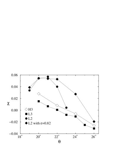
FIG. 16.: Dependence of the normal stress anomaly $\chi$ on tilt angle $\theta$ for Models L2 and L3 (closed symbols), and Model H3 (open symbols).

The fact that the stress varies linearly with depth and our earlier observations of constant density suggests that the analysis relevant to our systems is that due to Bagnold [1]. Bagnold’s collisional-momentum transfer analysis for granular systems works under the assumption of a constant density profile, resulting in stress profiles that vary linearly with depth. The essence of Bagnold’s theory is a constitutive equation whereby the shear stress $\sigma_{xz}$ is proportional to the square of the strain rate $\dot{\gamma}^{2}\equiv\left(\partial v_{x}(z)/\partial z\right)^{2}$, where $v_{x}(z)$ is the velocity in the direction of flow at height $z$:

$$\sigma_{xz}=A_{\rm Bag}^{2}{\dot{\gamma}}^{2}.$$ (21)

Combined with Eq.(18), and the no-slip boundary condition at $z=0$, this results in a velocity profile of the form,

$$v_{x}(z)=A_{\rm Bag}h^{3/2}\left(\frac{2}{3}\sqrt{\rho g\sin\theta}\right)\left[1-\left(\frac{h-z}{h}\right)^{3/2}\right].$$ (22)

From Fig. 17, we observe that for the bulk of the flow, the relationship $\sigma_{xz}\propto\dot{\gamma}^{2}$ holds to a good approximation below the first 5-8 layers, and away from the bottom wall, for the 2D and 3D systems. We have fitted the “Bagnold” scaling with the dotted lines, the solid lines and symbols represent the simulation data [43]. The tilt dependence of the overall amplitude of the strain rate, $A_{\rm Bag}$, is shown in Fig. 18. In 3D, $A_{\rm Bag}$ continuously approaches zero at the angle of repose, whereas in 2D, there is a jump in this amplitude, consistent with the overall hysteretic behavior.

(a) (b)

FIG. 17.: Rheology curves of chute flow systems-shear strain vs. shear stress; a) 2D, (Model L2, $H=100$) and b) 3D ($H=40$): Model L3 (symbols) and Model H3 (solid lines). Bagnold scaling fits in the bulk are shown by dashed lines for Model L and dotted lines for Model H.

FIG. 18.: Strain rate amplitude $A_{\rm Bag}=\dot{\gamma}/\sqrt{\sigma_{xz}}$ associated with the bulk Bagnold rheology for the three model systems. Whereas 3D amplitudes extrapolate to zero at $\theta_{r}$, there is a finite jump associated with the 2D amplitude at $\theta_{r}$.

Another way to test this scaling is by plotting the average velocity $<v^{2}>^{1/2}$ as a function of $H$ (which is proportional to $h$). The scaling in Fig. 19 shows that $<v^{2}>^{1/2}\propto H^{\alpha}$, where $\alpha=1.52\pm 0.05$. This result also agrees well with experiment [29]. If we rescale the data from Fig. 7, we find good agreement apart from the region near the top surface where the density is no longer constant. This suggests that Bagnold’s theory may provide an approximate description of the bulk motion of our systems. In fact, Bagnold scaling is a generic dimensional result for the situation where the time scale of the system is only set by the inverse of the shear rate, as is the case here [2].

Bagnold’s original stress-strain rate relationship arises from a momentum transfer mechanism that is based on binary collisions. From the simulation data, we find that the dominant term in the stress is due to lasting contacts between particles, and the ballistic (kinetic) contribution to the stress is significantly smaller (about $1\%$ of the total value). Thus, the success of the Bagnold scaling is based on the dimensional structure of the problem, rather than on the particular momentum transfer mechanism that he identified.

(a) (b)

FIG. 19.: Scaling of velocity in the direction of flow $<v^{2}_{x}(z)>^{1/2}$ with system height $H$ in; (a) 2D at $20^{o}$ with $\epsilon=0.92$, for two different values of $\mu$, (b) model H3 at $24^{o}$. The slope of the lines indicate that $<v^{2}>^{1/2}\propto H^{\alpha}$, with $\alpha=1.52\pm 0.05$.

Another method to test the nature of collisions is to compute the average coordination number $Z_{c}$ as a function of inclination angle. This data, for the 2D and 3D linear-spring systems, is shown in Fig. 20. In a system dominated by binary collisions, one would expect $Z_{c}\ll 1$; this is clearly not the case for our system. The observed behavior is an increasing $Z_{c}$ as $\theta$ approaches the angle of repose from above. Normalized this way for a static 2D triangular lattice with no free particles, the value would be 3. Similarly, for 3D static packings one might expect a value between $4-6$ [44].

Because of these observations, we reason that contributions to the kinetic term of the stress tensor do not play a significant role in determining the macroscopic quantities measured. It might then be argued that for a densely packed pile of stiff objects in motion, the overall time evolution of the system in the configurational phase space is primarily constrained and controlled by aspects of geometrical packing, rather than the specific form of the stiff force laws between particles or dissipation functions. This might be why the system is so insensitive to variations in the interaction parameters, as described in Sec. III B.

FIG. 20.: Averaged instantaneous coordination number $Z_{c}$,as a function of tilt angle for Model L2 with $H=100$, and Model L3 with $H=40$.

V Conclusions

We have concentrated on the steady-state nature of chute flows, specifying first the region in phase space in which such flows can be observed, and second the structure and rheology of these flows.

A region of constant packing fraction is a generic feature in our 2D and (two) 3D models, with only a small dilated layer at the free surface. Analysis of the velocity profiles has revealed that to a good approximation, Bagnold scaling holds: the Bagnold velocity profile, $v_{x}\propto H^{1.5}$, and rheology, $\sigma\propto\dot{\gamma}^{2}$, is reasonably verified away from the surface. This is in contrast with earlier simulations on chute flows, which indicated linear velocity profiles. We argue that although this latter may be the case for small systems, such as flowing layers less than 20 particles high, steady flows of moderately thick systems are well-approximated by Bagnold scaling.

Although the regime of Bagnold-like flow appears to dominate the system, we have found that deviations from this simple theory exist. The normal stress anomaly remains a mystery, and our fits to the stress-strain rate curves apply only away from the top and bottom surfaces. We have also found that the transmission of stress in such dense flows is dominated by contacts, as opposed to binary collisions in Bagnold’s analysis of dilute flows.

Finally, we observe that the normal stresses in bulk flows do not approach a Coulomb yield criterion structure at the angle of repose, despite the continuous disappearance of the shear rate at this threshold. The fact that Coulomb yield is approached at the surface for 3D flows hints at a special role for surface failure in this case.

Our simulation code, both in its simple and parallelised versions, enables us to study large systems for very long time scales, and we continue to investigate some of the outstanding issues in this area. We will report elsewhere the differences between rough and smooth bottom surfaces [3]. We will also go on to study 3D planar Couette flows, extending Ref. [45], and will be reporting on this in the future.

REFERENCES

- [1] R. A. Bagnold, Proc. Royal Society. London 255, 49 (1954).
- [2] D. Ertaş, G. S. Grest, T. C. Halsey, D. Levine, and L. E. Silbert, submitted to Europhysics Letters (unpublished).
- [3] L. E. Silbert, G. S. Grest, S. J. Plimpton, and D. Levine, in preparation (unpublished).
- [4] S.-S. Hsiau and H.-W. Jang, J. Chinese Institute Engineers 22, 93–99 (1999).
- [5] D. W. Howell, R. P. Behringer, and C. T. Veje, Chaos 9, 559–572 (1999).
- [6] A. Barois-Cazenave, P. Marchal, V. Falk, and L. Choplin, Powder Tech. 103, 58–64 (1999).
- [7] M. Medved, D. Dawson, H. M. Jaeger, and S. R. Nagel, Chaos 9, 691–696 (1999).
- [8] T. Takahashi, Ann. Rev. Fluid Mech. 13, 57–77 (1981).
- [9] C. S. Campbell, P. W. Cleary, and M. Hopkins, J. Geophysical Res. 100, 8267–8283 (1995).
- [10] J. T. Jenkins and E. Askari, Chaos 9, 654–658 (1999).
- [11] P.-A. Lemieux and D. J. Durian, Phys. Rev. Lett. 85, 4273–4276 (2000).
- [12] O. Pouliquen and N. Renaut, J. Phys. II 6, 923–935 (1996).
- [13] O. Hungr and N. R. Morgenstern, Gotechnique 3, 405–413 (1984).
- [14] T. G. Drake, J. Geophysical Res. 95, 8681–8696 (1990).
- [15] E. Azanza, F. Chevoir, and P. Moucheront, J. Fluid Mech. 400, 199–227 (1999).
- [16] D. M. Hanes and O. R. Walton, Powder Tech. 109, 133–144 (2000).
- [17] S. B. Savage, J. Fluid Mech. 377, 1–26 (1998).
- [18] H. Ahn, C. E. Brennen, and R. H. Sabersky, J. of Appl. Mech. 59, 109–119 (1992).
- [19] P. Mills, D. Loggia, and M. Tixier, Europhys. Lett. 45, 733–738 (1999).
- [20] D. V. Kharkhar, J. J. McCarthy, and J. M. Ottino, Powder Tech. 86, 219–227 (1996).
- [21] D. Hirshfield and D. C. Rapaport, Phys. Rev. E 56, 2012–2018 (1997).
- [22] O. R. Walton and R. L. Braun, J. Rheo. 30, 949–980 (1863).
- [23] O. R. Walton, Mech. Mat. 16, 239–247 (1993).
- [24] T. Pschel, J. Phys. II 3, 27–40 (1993).
- [25] X. M. Zheng and J. M. Hill, Powder Tech. 86, 219–227 (1996).
- [26] X. M. Zheng and J. M. Hill, Comp. Mech. 22, 160–166 (1998).
- [27] S. Dippel and D. E. Wolf, Computer Physics Communications 121-122, 284–289 (1999).
- [28] P. A. Cundall and O. D. L. Strack, Gotechnique 29, 47–65 (1979).
- [29] O. Pouliquen, Phys. Fluids 11, 542–548 (1999).
- [30] L. Vanel, D. Howell, D. Clark, R. P. Behringer, and E. Clement, Phys. Rev. E 60, R5040–R5043 (1999).
- [31] L. Vu-Quoc and X. Zhang, Mech. Mat. 31, 235–269 (1999).
- [32] B. C. Vemuri, L. C. L. Vu-Quoc, X. Zhang, and O. Walton, Mech. Mat. 31, 235–269 (1999).
- [33] J. J. Moreau, Euro. J. Mech. and Solids 13, 93–114 (1994).
- [34] We have also studied the role of dynamic friction in 2D simulations. This model has set to zero always, and only includes the tangential velocity damping term . Using this model, we never observed a steady state flow for our chute flow simulations.
- [35] T. C. Halsey and D. Ertaş, Phys. Rev. Lett. 83, 5007 (1999).
- [36] R. D. Mindlin and H. Deresiewicz, L. Appl. Mech. 20, 327 (1953).
- [37] K. L. Johnson, Contact Mechanics (Cambridge, UK, 1999).
- [38] J. Schafer, S. Dippel, and D. E. Wolf, J. Phys. I France 6, 5–20 (1996).
- [39] M. P. Allen and D. J. Tilldesley, Computer Simulations of Liquids (Oxford, UK, 1999).
- [40] S. J. Plimpton, J. Comp. Phys. 117, 1–19 (1995).
- [41] Although we do not see slip in this study, we have observed slip in our 2D simulations using a smoother bottom wall constructed from spheres of the same diameter as those in the bulk.
- [42] R. M. Nedderman, Statics and Kinematics of Granular Materials (Cambridge, UK, 1992).
- [43] Although the overall fit is good, deviations from the simple scaling law occur even at depths where the density has reached its bulk value. Thus, the rheology of the system does not appear to be entirely local, with surface effects penetrating farther into the pile than is suggested by the density profile.
- [44] H. A. Makse, D. L. Johnson, and L. M. Schwartz, Phys. Rev. Lett. 84, 4160–4163 (2000).
- [45] P. A. Thompson and G. S. Grest, Phys. Rev. Lett. 67, 1751–1754 (1991).