Spin waves in the spiral phase of a doped antiferromagnet: a strong-coupling approach

Abstract

We study spin fluctuations in the spiral phase of the two-dimensional Hubbard model at low doping on the basis of the spin-particle-hole coherent-state path integral. In the strong correlation limit, we obtain an analytical expression of the spin-wave excitations over the entire Brillouin zone except in the vicinity of ${\bf q}=0$. We discuss the validity of the Hartree-Fock and random-phase approximations in the strong-coupling limit, and compare our results with previous numerical and analytical calculations. Although the spiral phase is unstable, as shown by a negative mean-field compressibility and the presence of imaginary spin-fluctuation modes, we expect the short-wavelength fluctuation modes (with real energies) to survive in the actual ground-state of the system.

I Introduction

Despite a lot of theoretical efforts, there is still no satisfying description of the ground-state and the low-lying excitations of a doped two-dimensional (2D) antiferromagnet. One of the simplest (realistic) models describing such a system is the Hubbard model. In the strong correlation limit, it reduces to the Heisenberg model at half-filling. For a 2D square lattice, the ground-state is known to be antiferromagnetic, and the low-lying excitations (spin-waves) are well understood. However, away from half-filling, the coexistence of local moments and itinerant charge carriers raises difficulties that have not been overcome so far.

In the framework of the Heisenberg model, perturbation theory around a broken-spin-symmetry ground-state (from linear spin-wave analysis to renormalization-group approach) has proven to be very successful. Formally, this semiclassical approach corresponds to a $1/S$ expansion, where $S$ is the size of the localized spins. It is very natural to follow the same line of approach in itinerant spin-$\frac{1}{2}$ fermion systems by promoting the localized moments from spin-$\frac{1}{2}$ to spin-$S$ (with $S\gg 1$). The spin degrees of freedom are then treated semiclassically, whereas the itinerant fermions are considered quantum mechanically.

The semiclassical approach is realized for instance in the Hartree-Fock or random-phase (RPA) approximations. For the Hubbard model, the (homogeneous) Hartree-Fock theory [1, 2, 3, 4, 5, 6, 7, 8, 9, 10] and the slave-boson mean-field theory[3, 11] predict a spiral magnetic order at strong coupling in agreement with mean-field (semiclassical) theories of the $t$-$J$ model [12, 13, 14, 15, 16] as first shown by Schraiman and Siggia.[17] This (homogeneous) spiral phase turns out to be unstable, as shown by a negative compressibility. The instability also manifests itself by the presence of imaginary spin-wave modes. [5, 6, 8, 10] Short-range spiral order,[17], phase separation, coexisting spin- and charge-density waves (domain-wall formation), [18, 5, 6, 8] and formation of local spin polarons[19, 20, 21] have been proposed as a possible alternative to the spiral phase. Although phase separation is likely to be suppressed by long-range Coulomb interaction, it is not clear whether the latter can stabilize the homogeneous spiral magnetic order. [5, 6] In any case, we expect the short-range spiral order to survive in the actual ground-state of the system. The study of (short-wavelength) spin-wave modes around the mean-field spiral order can then be seen as a way to access this short-range order, even though the mean-field theory incorrectly predicts a long-range spiral order. On the experimental side, strong antiferromagnetic fluctuations have been observed in the normal phase of high-$T_{c}$ copper oxides. In particular, inelastic neutron scattering data have revealed noticeable incommensurate fluctuations at finite doping. [22]

In this paper, we reconsider the semiclassical limit of the 2D Hubbard model on the basis of the spin-particle-hole coherent-state path integral. [23, 24] The latter has been designed to study strongly correlated fermion systems where itinerant charge carriers interact with local moments. As shown below, it provides a very natural framework to derive the spin-wave modes around the mean-field spiral order.

The outline of the paper is as follows. In Sec. II, we introduce the effective action of the Hubbard model based on the spin-particle-hole coherent-state path integral. After performing a saddle-point approximation on the spin variables corresponding to a (homogeneous) spiral order, we calculate the hole Green’s function and the free energy within a $t/U$ expansion. We discuss the reason why the Hartree-Fock theory turns out to be correct in the strong correlation limit at low doping. In Sec. III, we compute the spin-wave excitations. We point out that a correct description of the three Goldstone modes of the spiral phase (at ${\bf q}=0,\pm{\bf Q}$, where ${\bf Q}$ is the wave-vector of the spin modulation) follows from a consistent calculation of vertex corrections and self-energy terms in the fermion Green’s functions. Finally, we obtain an analytical expression of the spin-wave excitations valid over the entire Brillouin zone, except in the vicinity of ${\bf q}=0$. We compare our analytical result with previous numerical [5, 6, 8, 9] and analytical calculations.[10]

II Mean-field theory

We consider a bipartite 2D lattice with $N$ sites. The Hubbard model is defined by

$$\hat{H}=-t\sum_{\langle{\bf r},{\bf r}^{\prime}\rangle,\sigma}(\hat{c}^{\dagger}_{{\bf r}\sigma}\hat{c}_{{\bf r}^{\prime}\sigma}+{\rm h.c.})+U\sum_{\bf r}\hat{n}_{{\bf r}\uparrow}\hat{n}_{{\bf r}\downarrow},$$ (1)

where $\hat{c}_{{\bf r}\sigma}$ is a fermionic operator for a $\sigma$-spin particle at site $\bf r$ ($\sigma=\uparrow,\downarrow$), $\hat{n}_{{\bf r}\sigma}=\hat{c}^{\dagger}_{{\bf r}\sigma}\hat{c}_{{\bf r}\sigma}$, and $\langle{\bf r},{\bf r}^{\prime}\rangle$ denotes nearest neighbors. We denote by $\mu$ the chemical potential, $\beta$ the inverse temperature, and $n=1-x$ the mean number of particles per site. We consider only hole doping ($x\geq 0$) and set $\hbar=k_{B}=1$ throughout the paper. All results are obtained in the zero-temperature limit ($T\to 0$).

The spin-particle-hole coherent-state path integral formulation of the Hubbard model was derived in Refs. [23, 24]. This approach is based on the introduction of spin-particle-hole coherent states which generalize the spin-$\frac{1}{2}$ coherent states by allowing the creation of a hole or an additional particle. In the strong-coupling limit $U\gg t$, the effective action $S[\gamma^{*},\gamma;{\bf\Omega}]$ of the Hubbard model is given by

$$S[\gamma^{*},\gamma;{\bf\Omega}] = \sum_{\bf r}\int d\tau\gamma^{*}_{{\bf r}\uparrow}(\partial_{\tau}-\mu+A^{0}_{\bf r})\gamma_{{\bf r}\uparrow}-\sum_{{\bf r},{\bf r}^{\prime}}\int d\tau\gamma^{*}_{{\bf r}\uparrow}\hat{t}_{{\bf r}\uparrow,{\bf r}^{\prime}\uparrow}\gamma_{{\bf r}^{\prime}\uparrow}$$ (5)

$$+\sum_{\bf r}\int d\tau\gamma^{*}_{{\bf r}\downarrow}(\partial_{\tau}-\mu+U-A^{0}_{\bf r})\gamma_{{\bf r}\downarrow}-\sum_{{\bf r},{\bf r}^{\prime}}\int d\tau\gamma^{*}_{{\bf r}\downarrow}\hat{t}_{{\bf r}\downarrow,{\bf r}^{\prime}\downarrow}\gamma_{{\bf r}^{\prime}\downarrow}$$

$$-\sum_{{\bf r},{\bf r}^{\prime}}\int d\tau\Bigl{(}\gamma^{*}_{{\bf r}\uparrow}\hat{t}_{{\bf r}\uparrow,{\bf r}^{\prime}\downarrow}\gamma_{{\bf r}^{\prime}\downarrow}+{\rm c.c.}\Bigr{)}$$

$$+\sum_{\bf r}\int d\tau_{1}d\tau_{2}d\tau_{3}d\tau_{4}\Gamma^{\rm II}_{\uparrow\downarrow,\uparrow\downarrow}(\tau_{1},\tau_{2};\tau_{3},\tau_{4})\gamma^{*}_{{\bf r}\uparrow}(\tau_{1})\gamma^{*}_{{\bf r}\downarrow}(\tau_{2})\gamma_{{\bf r}\downarrow}(\tau_{4})\gamma_{{\bf r}\uparrow}(\tau_{3}).$$

${\bf\Omega}$ is a unit vector field which gives the direction of the local moments at the singly-occupied sites. $\gamma_{\uparrow}$ and $\gamma_{\downarrow}$ are Grassmann variables describing particles propagating in the lower (LHB) and upper (UHB) Hubbard bands, respectively. $A^{0}_{\bf r}=\langle{\bf\Omega}_{\bf r}|\dot{\bf\Omega}_{\bf r}\rangle$ is a Berry phase term ($|\dot{\bf\Omega}_{\bf r}\rangle=\partial_{\tau}|{\bf\Omega}_{\bf r}\rangle$). The intersite hopping matrix $\hat{t}_{{\bf r}{\bf r}^{\prime}}=R^{\dagger}_{\bf r}t_{{\bf r}{\bf r}^{\prime}}R_{{\bf r}^{\prime}}$ depends on ${\bf\Omega}$ via the SU(2)/U(1) matrix

$$R_{\bf r}=e^{-\frac{i}{2}\varphi_{\bf r}\sigma_{z}}e^{-\frac{i}{2}\theta_{\bf r}\sigma_{y}}e^{-\frac{i}{2}\psi_{\bf r}\sigma_{z}}$$ (6)

which rotates the unit vector $\hat{\bf z}$ to ${\bf\Omega}_{\bf r}={\bf\Omega}(\theta_{\bf r},\varphi_{\bf r})$. Here $\theta_{\bf r}$ and $\varphi_{\bf r}$ are the polar angles determining the direction of ${\bf\Omega}_{\bf r}$. The choice of $\psi_{\bf r}$ is free and corresponds to a “gauge” freedom. In the Hubbard model, $t_{{\bf rr}^{\prime}}=t$ if ${\bf r}$ and ${\bf r}^{\prime}$ are nearest neighbors and vanishes otherwise. The quartic term of the action (5) is determined by the two-particle atomic vertex $\Gamma^{\rm II}$.

In this section, we make a saddle-point approximation on the spin variables ${\bf\Omega}_{\bf r}$. As discussed in Ref. [24], this approach can be justified by taking a “large-$S$” semiclassical limit, which consists in promoting the spin-$\frac{1}{2}$ coherent states describing singly occupied sites to spin-$S$ coherent states. In the limit $S\to\infty$, the Berry phase term suppresses quantum fluctuations of ${\bf\Omega}$. The spin variables become classical and do not fluctuate at zero temperature.

A broken-symmetry ground-state corresponding to a (coplanar) spiral order is defined by the “classical” configuration

$$\theta^{\rm cl}_{\bf r}=\frac{\pi}{2},\,\,\,\,\,\,\,\,\,\varphi^{\rm cl}_{\bf r}={\bf Q}\cdot{\bf r}.$$ (7)

We consider only the diagonal spiral phase (${\bf Q}=(Q,Q)$), which is known to be the most stable one in the strong-coupling limit.[1] Note that the antiferromagnetic (${\bf Q}=(\pi,\pi)$) and ferromagnetic (${\bf Q}=0$) phases are special cases of the spiral order defined by Eq. (7). In the gauge $\psi_{\bf r}=0$, the hopping matrix $\hat{t}^{\rm cl}_{{\bf r}{\bf r}^{\prime}}$ depends only on the difference ${\bf r}-{\bf r}^{\prime}$:

$$\hat{t}^{\rm cl}_{{\bf r}{\bf r}^{\prime}}=t_{{\bf r}{\bf r}^{\prime}}e^{-\frac{i}{2}{\bf Q}\cdot({\bf r}-{\bf r}^{\prime})\sigma_{x}}.$$ (8)

This yields the following saddle-point action:

$$S_{\rm cl}[\gamma^{*},\gamma] = -\sum_{{\bf k},\omega,\sigma}\gamma^{*}_{{\bf k}\sigma}(i\omega)(i\omega+\mu-U\delta_{\sigma\downarrow}+2t\cos\frac{Q}{2}\cos k_{\nu})\gamma_{{\bf k}\sigma}(i\omega)+\sum_{{\bf k},\omega,\sigma}\gamma^{*}_{{\bf k}\sigma}(i\omega)2t\sin\frac{Q}{2}\sin k_{\nu}\gamma_{{\bf k}\bar{\sigma}}(i\omega)$$ (10)

$$+\frac{1}{N\beta}\sum_{{\bf k},{\bf k}^{\prime},{\bf q}}\sum_{\omega_{1},\omega_{2},\omega_{3}}\Gamma^{\rm II}_{\uparrow\downarrow,\uparrow\downarrow}(i\omega_{1},i\omega_{2};i\omega_{3}(i\omega_{4}))\gamma^{*}_{{\bf k}+{\bf q}\uparrow}(i\omega_{1})\gamma^{*}_{{\bf k}^{\prime}-{\bf q}\downarrow}(i\omega_{2})\gamma_{{\bf k}^{\prime}\downarrow}(i\omega_{4})\gamma_{{\bf k}\uparrow}(i\omega_{3}),$$

where $\gamma_{{\bf k}\sigma}$ is the Fourier transform of $\gamma_{{\bf r}\sigma}$, and ${\bf k}$ runs over the entire Brillouin zone. $\Gamma^{\rm II}_{\uparrow\downarrow,\uparrow\downarrow}(i\omega_{1},i\omega_{2};\omega_{3}(i\omega_{4}))=i\omega_{2}-i\omega_{3}-U$, where $\omega_{4}=\omega_{1}+\omega_{2}-\omega_{3}$ is fixed by energy conservation. In Eq. (10) and below, there is an implicit sum over $\nu=x,y$. Without the quartic term, the action (10) is similar to that obtained in Refs. [5, 6] within a large-$U$ Hartree-Fock approximation where the SU(2) spin-rotation invariance is maintained by introducing a fluctuating spin-quantization axis in the functional integral. We show below that the quartic term can indeed be neglected in the low-doping limit.

For later convenience, we introduce the parameter

$$p=-\cos\frac{Q}{2}\geq 0$$ (11)

which determines the spiral pitch. By changing $Q$ in $Q+2\pi$, it is always possible to choose the sign of $p$ positive. $p$ varies from 0 in the antiferromagnetic phase to 1 in the ferromagnetic phase.

FIG. 1.: Definition of the various symbols appearing in the Feynman diagrams.

FIG. 2.: Diagrammatic representation of the LHB self-energy at order $O(t/U)$. Slashed dashed lines indicate interband transitions ($\hat{t}^{\rm cl}_{\sigma\bar{\sigma}}$).

We are now in a position to apply the strong-coupling perturbation theory described in Ref. [24]. We first consider the LHB Green’s function. To zeroth order in $t/U$, $\hat{t}^{\rm cl}_{\sigma\bar{\sigma}}$ is ignored, since it corresponds to interband transitions. As shown in Ref. [24], $\Gamma^{\rm II}$ does not affect the LHB Green’s function to this order. We thus obtain

$${\cal G}^{(0)}_{\uparrow}({\bf k},i\omega)=(i\omega+\mu-2tp\cos k_{\nu})^{-1}$$ (12)

as the propagator of the $\gamma_{\uparrow}$ field. Corrections to ${\cal G}^{(0)}_{\uparrow}$ are taken into account by introducing a self-energy $\Sigma$, i.e. ${\cal G}^{-1}_{\uparrow}={\cal G}^{(0)-1}_{\uparrow}-\Sigma$. To order $O(t/U)$, there are three contributions to $\Sigma$ shown in Fig. 2.[24] [The symbols used in the Feynman diagrams are defined in Fig. 1.] The last contribution (Fig. 2c) vanishes due to the sum over the internal momentum in the loop. We show at the end of this section that the second contribution (Fig. 2b) can be neglected in the low-doping limit. The first contribution (Fig. 2a) gives

$$\Sigma({\bf k},i\omega) = 4t^{2}(1-p^{2})(\sin k_{\nu})^{2}G^{(0)}_{\downarrow}(i\omega)$$ (13)

$$\simeq -J(1-p^{2})(\sin k_{\nu})^{2},$$ (14)

where $J=4t^{2}/U$. The last line of Eq. (14) is obtained by approximating the UHB atomic Green’s function $G^{(0)}_{\downarrow}(i\omega)=(i\omega+\mu-U)^{-1}$ by $-1/U$. We therefore obtain the following expression for the propagator of the $\gamma$ field:

$${\cal G}_{\uparrow}({\bf k},i\omega)=(i\omega-\epsilon_{\bf k})^{-1},$$ (15)

$$\epsilon_{\bf k}=-\mu+2tp\cos k_{\nu}-J(1-p^{2})(\sin k_{\nu})^{2}.$$ (16)

It should be noted that ${\cal G}_{\uparrow}$ is not the LHB Green’s function of the original fermions (i.e. the $c$ field in Eq. (1)). The latter is given by (see Eq. (3.32) in Ref. [24])

$${\cal G}^{\rm LHB}_{\sigma}({\bf r}\tau,{\bf r}^{\prime}\tau^{\prime}) = (R_{\bf r}(\tau))_{\sigma\uparrow}{\cal G}_{\uparrow}({\bf r}\tau,{\bf r}^{\prime}\tau^{\prime})(R_{\bf r}^{\prime}(\tau^{\prime}))_{\uparrow\sigma}$$ (17)

$$= \frac{e^{-\frac{i}{2}\sigma{\bf Q}\cdot({\bf r}-{\bf r}^{\prime})}}{2}{\cal G}_{\uparrow}({\bf r}\tau,{\bf r}^{\prime}\tau^{\prime}).$$ (18)

In Fourier space, this gives

$${\cal G}^{\rm LHB}_{\sigma}({\bf k},i\omega)=\frac{1}{2}{\cal G}_{\uparrow}({\bf k}+\frac{\sigma}{2}{\bf Q},i\omega).$$ (19)

The quasi-particle pole has a residue equal to $1/2$, as expected since ${\cal G}^{\rm LHB}_{\sigma}$ is the Green’s function projected onto the LHB. Moreover, the dispersion law of the original fermions is shifted by $\pm{\bf Q}/2$ with respect to that of the $\gamma_{\uparrow}$ particles.

Eqs. (16) and (19) agrees with the large-$U$ expansion of the Hartree-Fock result. There are two contributions to the energy $\epsilon_{\bf k}$ of the particles in the LHB. The first is due to inter-sublattice hopping processes and gives a band of width $8tp$. The second comes from intra-sublattice hopping processes which occur via virtual transitions to the UHB. The resulting bandwidth is of order $J(1-p^{2})$. Anticipating that $p\simeq(U/2t)x$ [Eq. (30)], inter- (intra)-sublattice hopping processes dominate when $J(1-p^{2})\ll tp$, i.e $t^{2}/U^{2}\ll x$ ($tp\ll J(1-p^{2})$, i.e. $x\ll t^{2}/U^{2}$). From Eq. (16), we readily see the instability of the antiferromagnetic phase against the formation of a spiral phase in the presence of holes. When $p$ is finite, the kinetic energy gain due to inter-sublattice hopping (or order $p$) dominates over the energy loss due to intra-sublattice hopping (of order $p^{2}$), thus stabilizing a non-linear spin order. [Note that the energy loss due to intra-sublattice hopping can also be seen as a loss of exchange energy.]

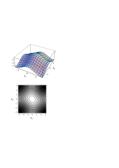
FIG. 3.: Dispersion law $\epsilon_{\bf k}$ in the LHB for $t^{2}/U^{2}\ll x$ ($U/t=10$ and $x=0.15$).

Since $p\geq 0$, the top of the LHB (for the $\gamma$ particles) is located in the middle of the Brillouin zone (${\bf k}=0$). In the vicinity of ${\bf k}=0$, the dispersion law (16) can be approximated as

$$\epsilon_{\bf k}\simeq-\mu+4tp-tpk^{2}-J(1-p^{2})(k_{x}+k_{y})^{2}.$$ (20)

Introducing the momentum ${\bf K}$ defined by

$$K_{x}=\frac{k_{x}+k_{y}}{\sqrt{2}},\,\,\,\,\,\,K_{y}=\frac{-k_{x}+k_{y}}{\sqrt{2}},$$ (21)

we obtain a parabolic band with anisotropic effective masses:

$$\epsilon_{\bf K} = -\mu+4tp-\frac{K_{x}^{2}}{2m_{x}}-\frac{K_{y}^{2}}{2m_{y}},$$ (22)

$$\frac{1}{m_{x}} = 2tp+4J(1-p^{2}),\,\,\,\,\,\,\,\,\frac{1}{m_{y}}=2tp.$$ (23)

The dispersion law $\epsilon_{\bf k}$ is shown in Figs. 3 and 4 (we have used $p\simeq(U/2t)x$, see Eq. (30)). When $t^{2}/U^{2}\ll x$, the anisotropy of the effective masses is weak and the Fermi surface is almost circular. The minima of the LHB lie at the corners of the Brillouin zone (Fig. 3). With decreasing $x$, the Fermi surface becomes elliptical, and the minima of the LHB move away from the corners of the Brillouin zone (Fig. 4).

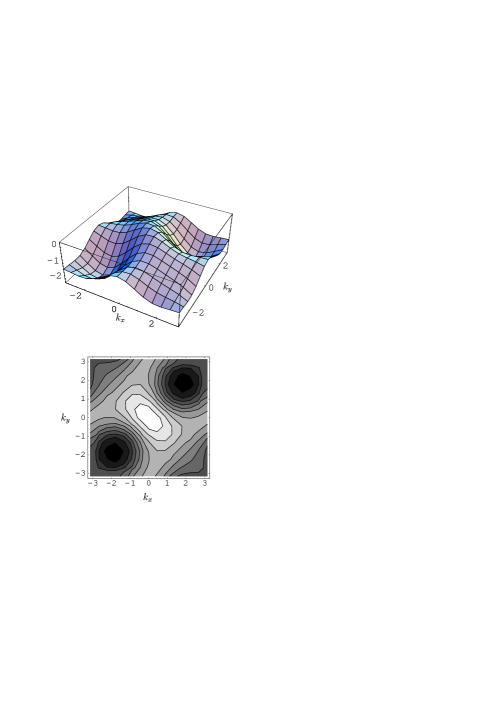
FIG. 4.: Dispersion law $\epsilon_{\bf k}$ in the LHB for $x\sim t^{2}/U^{2}$ ($U/t=10$ and $x=0.04$).

For $T=0$, the free energy (per site) $F(\mu)$ is given by (see Appendix A)

$$F = \frac{1}{N}\sum_{\bf k}\theta(-\epsilon_{\bf k})\epsilon_{\bf k}$$ (24)

$$= -\mu-J(1-p^{2})-\frac{(4tp-\mu)^{2}}{4\pi}\sqrt{m_{x}m_{y}}.$$ (25)

The chemical potential is obtained from $n=1-x=-\partial F/\partial\mu$,[25] i.e.

$$\mu=4tp-\frac{2\pi x}{\sqrt{m_{x}m_{y}}}.$$ (26)

From Eqs. (25) and (26), we deduce the energy $E(x)=F+\mu(1-x)$:

$$E=-4tpx-J(1-p^{2})+\frac{\pi x^{2}}{\sqrt{m_{x}m_{y}}}.$$ (27)

The spiral pitch is obtained by minimizing the energy $E$ at fixed hole doping $x$, i.e. $\partial E/\partial p=0$. This gives the following equation for $p$:

$$(4tx-2Jp)[4t^{2}p^{2}+8tJp(1-p^{2})]^{1/2}$$ (28)

$$=\frac{\pi x^{2}}{2}[8t^{2}p+8tJ(1-3p^{2})].$$ (29)

In the limit $x\ll 1$, we find[26, 5, 6, 10]

$$p\simeq\frac{U}{2t}x.$$ (30)

At half-filling, the spin configuration is antiferromagnetic ($p=0$). As soon as holes are introduced into the system, a spiral phase is stabilized. Since $p\leq 1$, Eq. (30) holds only when $x\leq x_{c}=2t/U$. When $x\geq x_{c}$, the minimum of the energy is reached for the ferromagnetic state ($p=1$).

From Eqs. (26) and (30), we deduce that the compressibility $\kappa=\partial n/\partial\mu\simeq-1/2U$ is negative in the spiral phase. This signals an instability towards phase separation. The presence of imaginary spin-wave modes at finite momenta (see Sec. III) suggests that other types of ground-states could also be stabilized. Zhou and Schulz have proposed a charge-density wave (coexisting with some kind of magnetic order). [5, 6] This possibility has also been studied in the framework of the Schraiman and Siggia’s model. [18] The ferromagnetic phase, which has a positive compressibility $\kappa\simeq 1/4\pi t$, is found to be stable.

FIG. 5.: Lowest-order correction $F^{\prime}$ to the free energy $F$ due to the two-particle vertex $\Gamma^{\rm II}$.

Let us now consider the self-energy shown in Fig. 2b. Although its calculation presents no difficulty, the determination of its contribution to the free energy requires to perform a coupling constant integration in order to ensure a consistent description of the system thermodynamics. Instead of considering $\Sigma$, we evaluate the lowest order correction $F^{\prime}$ to the free energy $F$ due to the two-particle vertex $\Gamma^{\rm II}$ (Fig. 5). This is sufficient to show that $\Gamma^{\rm II}$ can be ignored in the low-doping limit ($x\ll 1$). As shown in Appendix B, one finds

$$F^{\prime}=xJ(1-p^{2}).$$ (31)

$F^{\prime}$ can be simply taken into account by replacing $J(1-p^{2})$ in Eq. (25) by $J(1-p^{2})(1-x)$. This modification can be ignored for $x\ll 1$. We conclude that $\Gamma^{\rm II}$ can be ignored in the low-doping limit.

The fact that we can neglect the quartic term of the action $S[\gamma^{*},\gamma;{\bf\Omega}]$ justifies the functional integral formulation of Refs. [5, 6]. It is also the reason why a standard RPA analysis [3, 4, 5, 6, 8, 9, 10] gives correct results in the strong-coupling limit. Note however that this conclusion holds only in the low-doping limit ($x\ll 1$). For an arbitrary doping, the quartic term of the action (10) cannot be neglected, and the RPA approach breaks down since it misses processes of order $O(t/U)$. It should also be noted that the UHB Green’s function ${\cal G}_{\downarrow}$ obtained by diagonalizing the quadratic part of the action (10) (which is the starting point of the RPA approach) is meaningless in the strong-coupling regime since it does not correspond to the leading term within a $t/U$ expansion (see Ref. [24] for a detailed discussion of this point).

III Spin-wave modes

A Effective action

In this section, we derive the effective action for the fluctuations $\delta{\bf\Omega}_{\bf r}={\bf\Omega}_{\bf r}-{\bf\Omega}^{\rm cl}_{\bf r}$ of the spin variables around their saddle-point value. The calculation is performed within a perturbative expansion in $t/U$.

We parametrize the fluctuations $\delta{\bf\Omega}_{\bf r}$ by [27]

$$p_{\bf r}=\frac{1}{2}\delta{\bf\Omega}_{\bf r}\cdot\hat{\mathchoice{{\hbox{\boldmath$\displaystyle\theta$}}}{{\hbox{\boldmath$\textstyle\theta$}}}{{\hbox{\boldmath$\scriptstyle\theta$}}}{{\hbox{\boldmath$\scriptscriptstyle\theta$}}}}_{\bf r},\,\,\,\,\,\,q_{\bf r}=\delta{\bf\Omega}_{\bf r}\cdot\hat{\mathchoice{{\hbox{\boldmath$\displaystyle\varphi$}}}{{\hbox{\boldmath$\textstyle\varphi$}}}{{\hbox{\boldmath$\scriptstyle\varphi$}}}{{\hbox{\boldmath$\scriptscriptstyle\varphi$}}}}_{\bf r},$$ (32)

where $\hat{\mathchoice{{\hbox{\boldmath$\displaystyle\theta$}}}{{\hbox{\boldmath$\textstyle\theta$}}}{{\hbox{\boldmath$\scriptstyle\theta$}}}{{\hbox{\boldmath$\scriptscriptstyle\theta$}}}}_{\bf r}=\hat{\bf z}$ and $\hat{\mathchoice{{\hbox{\boldmath$\displaystyle\varphi$}}}{{\hbox{\boldmath$\textstyle\varphi$}}}{{\hbox{\boldmath$\scriptstyle\varphi$}}}{{\hbox{\boldmath$\scriptscriptstyle\varphi$}}}}_{\bf r}=(-\sin({\bf Q}\cdot{\bf r}),\cos({\bf Q}\cdot{\bf r}),0)$. $q_{\bf r}$ ($p_{\bf r}$) corresponds to fluctuations in (out of) the spiral plane. We easily obtain

$$p_{\bf r}=\frac{\cos\theta_{\bf r}}{2},\,\,\,\,\,\,q_{\bf r}\simeq\varphi_{\bf r}-{\bf Q}\cdot{\bf r},$$ (33)

where the last equality holds for small fluctuations. The Berry phase term can be expressed in terms of the variables $p,q$:

$$A^{0}_{\bf r}=-\frac{i}{2}(p_{\bf r}\dot{q}_{\bf r}-\dot{p}_{\bf r}q_{\bf r}).$$ (34)

Using Eqs. (6) and (33), we deduce

$$\delta\hat{t}_{{\bf rr}^{\prime}}=\hat{t}_{{\bf rr}^{\prime}}-\hat{t}^{\rm cl}_{{\bf rr}^{\prime}}=t_{{\bf rr}^{\prime}}\left(\begin{array}[]{lr}A_{{\bf rr}^{\prime}}&-B^{*}_{{\bf rr}^{\prime}}\\ B_{{\bf rr}^{\prime}}&A^{*}_{{\bf rr}^{\prime}}\end{array}\right)$$ (35)

where

$$A_{{\bf rr}^{\prime}} = \cos\biggl{(}\frac{{\bf Q}\cdot({\bf r}-{\bf r}^{\prime})}{2}\biggr{)}\biggl{[}-\frac{(p_{\bf r}-p_{{\bf r}^{\prime}})^{2}}{2}+\frac{i}{2}(p_{\bf r}+p_{{\bf r}^{\prime}})(q_{\bf r}-q_{{\bf r}^{\prime}})-\frac{(q_{\bf r}-q_{{\bf r}^{\prime}})^{2}}{8}\biggr{]}$$ (37)

$$+\sin\biggl{(}\frac{{\bf Q}\cdot({\bf r}-{\bf r}^{\prime})}{2}\biggr{)}\biggl{[}i(p_{\bf r}+p_{{\bf r}^{\prime}})-\frac{q_{\bf r}-q_{{\bf r}^{\prime}}}{2}\biggr{]},$$

$$B_{{\bf rr}^{\prime}} = \cos\biggl{(}\frac{{\bf Q}\cdot({\bf r}-{\bf r}^{\prime})}{2}\biggr{)}\biggl{[}p_{\bf r}-p_{{\bf r}^{\prime}}-\frac{i}{2}(q_{\bf r}-q_{{\bf r}^{\prime}})\biggr{]}$$ (39)

$$+\sin\biggl{(}\frac{{\bf Q}\cdot({\bf r}-{\bf r}^{\prime})}{2}\biggr{)}\biggl{[}\frac{i}{2}(p_{\bf r}+p_{{\bf r}^{\prime}})^{2}-\frac{1}{2}(p_{\bf r}-p_{{\bf r}^{\prime}})(q_{\bf r}-q_{{\bf r}^{\prime}})+\frac{i}{8}(q_{\bf r}-q_{{\bf r}^{\prime}})^{2}\biggr{]}$$

to quadratic order in $p,q$.

Taking into account spin fluctuations, the action can be written as

$$S[\gamma^{*},\gamma;{\bf\Omega}] = S_{\rm cl}[\gamma^{*},\gamma]-\sum_{{\bf r},{\bf r}^{\prime}}\int d\tau\gamma^{\dagger}_{\bf r}\delta\hat{t}_{{\bf rr}^{\prime}}\gamma_{{\bf r}^{\prime}}$$ (41)

$$+\sum_{{\bf r},\sigma}\sigma\int d\tau A^{0}_{\bf r}\gamma^{*}_{{\bf r}\sigma}\gamma_{{\bf r}\sigma},$$

where $\gamma_{\bf r}=(\gamma_{{\bf r}\uparrow},\gamma_{{\bf r}\downarrow})^{T}$. The action of the spin degrees of freedom is obtained by integrating out the fermions:

$$e^{-S[p,q]}=\int{\cal D}[\gamma]e^{-S[\gamma^{*},\gamma;{\bf\Omega}]}.$$ (42)

For small fluctuations around the classical configuration ${\bf\Omega}^{\rm cl}$, it is sufficient to determine $S[p,q]$ to quadratic order in $p,q$. We find

$$S[p,q]=S_{B}[p,q]+S_{1}[p,q]+S_{2}[p,q],$$ (43)

where

$$S_{B} = \sum_{{\bf r},\sigma}\sigma\int d\tau A^{0}_{\bf r}\langle\gamma^{*}_{{\bf r}\sigma}\gamma_{{\bf r}\sigma}\rangle_{\rm cl},$$ (44)

$$S_{1} = -\sum_{{\bf r},{\bf r}^{\prime}}\int d\tau\langle\gamma^{\dagger}_{\bf r}\delta\hat{t}_{{\bf rr}^{\prime}}\gamma_{{\bf r}^{\prime}}\rangle_{\rm cl},$$ (45)

$$S_{2} = -\frac{1}{2}\sum_{{\bf r}_{1},{\bf r}^{\prime}_{1},{\bf r}_{2},{\bf r}^{\prime}_{2}}\int d\tau_{1}d\tau_{2}\langle\gamma^{\dagger}_{{\bf r}_{1}}\delta\hat{t}_{{\bf r}_{1}{\bf r}^{\prime}_{1}}(\tau_{1})\gamma_{{\bf r}^{\prime}_{1}}$$ (47)

$$\times\gamma^{\dagger}_{{\bf r}_{2}}\delta\hat{t}_{{\bf r}_{2}{\bf r}^{\prime}_{2}}(\tau_{2})\gamma_{{\bf r}^{\prime}_{2}}\rangle_{\rm cl}.$$

$\langle\cdots\rangle_{\rm cl}$ means that the average is taken with the saddle-point action $S_{\rm cl}[\gamma^{*},\gamma]$, only the connected part being considered. $S_{B}$ is a Berry phase term, $S_{1}$ a first-order cumulant, and $S_{2}$ a second-order cumulant. Note that $A^{0}$ does not contribute to the second-order cumulant, since it is of second order in $p,q$.

1 Berry phase term $S_{B}$

Since $\langle\gamma^{*}_{{\bf r}\sigma}\gamma_{{\bf r}\sigma}\rangle_{\rm cl}=(1-x)\delta_{\sigma,\uparrow}$, we obtain

$$S_{B}=-\frac{i}{2}(1-x)\sum_{\bf r}\int d\tau(p_{\bf r}\dot{q}_{\bf r}-\dot{p}_{\bf r}q_{\bf r}).$$ (49)

$S_{B}$ is the standard expression for the Berry phase term of localized spins, with a reduction factor $1-x$ due to doping.

2 First-order cumulant $S_{1}$

We write the first-order cumulant as $S_{1}=S_{1}^{\prime}+S_{1}^{\prime\prime}$ where $S_{1}^{\prime}$ ($S^{\prime\prime}_{1}$) is of order $O(1)$ ($O(t/U)$). The corresponding Feynman diagrams are shown in Fig. 6. We find

$$S_{1}^{\prime} = -\sum_{{\bf r},{\bf r}^{\prime}}\int d\tau\delta\hat{t}_{{\bf r}\uparrow,{\bf r}^{\prime}\uparrow}{\cal G}_{\uparrow}({\bf r}^{\prime}-{\bf r},\tau=0^{-})$$ (50)

$$= -\frac{1}{\beta}\sum_{{\bf k},\omega}\delta\hat{t}_{{\bf k}\uparrow,{\bf k}\uparrow}{\cal G}_{\uparrow}({\bf k},i\omega),$$ (51)

$$S_{1}^{\prime\prime} = -\sum_{{\bf r},{\bf r}^{\prime},\sigma}\int d\tau\delta\hat{t}_{{\bf r}\sigma,{\bf r}^{\prime}\bar{\sigma}}{\cal G}_{\bar{\sigma}\sigma}({\bf r}^{\prime}-{\bf r},\tau=0^{-})$$ (52)

$$= -\frac{1}{\beta}\sum_{{\bf k},\omega.\sigma}\delta\hat{t}_{{\bf k}\sigma,{\bf k}\bar{\sigma}}{\cal G}_{\bar{\sigma}\sigma}({\bf k},i\omega),$$ (53)

where we have introduced

$$\delta\hat{t}_{{\bf k}\sigma,{\bf k}^{\prime}\sigma^{\prime}}=\frac{1}{N}\sum_{{\bf r},{\bf r}^{\prime}}e^{-i{\bf k}\cdot{\bf r}+i{\bf k}^{\prime}\cdot{\bf r}^{\prime}}\delta\hat{t}_{{\bf r}\sigma,{\bf r}^{\prime}\sigma^{\prime}}.$$ (54)

The Green’s function ${\cal G}_{\uparrow}({\bf k},i\omega)$ is given by Eq. (15). To first order in $t/U$,

$${\cal G}_{\bar{\sigma}\sigma}({\bf k},i\omega) = 2t\sin\frac{Q}{2}X_{\bf k}{\cal G}_{\uparrow}({\bf k},i\omega)G^{(0)}_{\downarrow}(i\omega)$$ (55)

$$\simeq -\frac{2t}{U}\sin\frac{Q}{2}X_{\bf k}{\cal G}_{\uparrow}({\bf k},i\omega),$$ (56)

where $X_{\bf k}=\sin k_{\nu}$.

FIG. 6.: Diagrammatic representation of $S_{1}^{\prime}$ and $S_{1}^{\prime\prime}$.

Performing the sums over the Matsubara frequencies and using

$$\delta\hat{t}_{{\bf k}\uparrow,{\bf k}\uparrow} = \frac{4t}{\sqrt{N}}\sin\frac{Q}{2}X_{\bf k}p_{{\bf q}=0}$$ (59)

$$-\frac{2t}{N}\cos\frac{Q}{2}\sum_{\bf q}\biggl{(}|p_{\bf q}|^{2}+\frac{|q_{\bf q}|^{2}}{4}\biggr{)}(Y_{\bf k}-Y_{{\bf k}+{\bf q}})$$

$$+i\frac{t}{N}\cos\frac{Q}{2}\sum_{\bf q}p_{\bf q}q_{-\bf q}(Y_{{\bf k}+{\bf q}}-Y_{{\bf k}-{\bf q}}),$$

$$\sum_{\sigma}\delta\hat{t}_{{\bf k}\sigma,{\bf k}\bar{\sigma}} = \frac{4t}{N}\sin\frac{Q}{2}\sum_{\bf q}\Bigl{[}|p_{\bf q}|^{2}(X_{\bf k}+X_{{\bf k}+{\bf q}})$$ (61)

$$+\frac{|q_{\bf q}|^{2}}{4}(X_{\bf k}-X_{{\bf k}+{\bf q}})\Bigr{]},$$

we finally obtain

$$S^{\prime}_{1} = -\frac{2tp}{N}\sum_{{\bf k},\tilde{q}}\theta(-\epsilon_{\bf k})(Y_{\bf k}-Y_{{\bf k}+{\bf q}})\biggl{(}|p_{\tilde{q}}|^{2}+\frac{|q_{\tilde{q}}|^{2}}{4}\biggr{)},$$ (62)

$$S^{\prime\prime}_{1} = \frac{2J(1-p^{2})}{N}\sum_{{\bf k},\tilde{q}}\theta(-\epsilon_{\bf k})X_{\bf k}\Bigl{[}|p_{\tilde{q}}|^{2}(X_{\bf k}+X_{{\bf k}+{\bf q}})$$ (64)

$$+\frac{|q_{\tilde{q}}|^{2}}{4}(X_{\bf k}-X_{{\bf k}+{\bf q}})\Bigr{]}.$$

where $Y_{\bf k}=\cos k_{\nu}$. Here we use the notation $\tilde{q}=({\bf q},i\omega_{\nu})$ with $\omega_{\nu}$ a bosonic Matsubara frequency. $p_{\tilde{q}}$ and $q_{\tilde{q}}$ are the Fourier transforms of $p_{\bf r}$ and $q_{\bf r}$ with respect to space and time.

3 Second-order cumulant $S_{2}$

We decompose $S_{2}$ into two contributions, $S_{2}^{\prime}$ and $S_{2}^{\prime\prime}$, which are represented diagrammatically in Fig. 7. $S_{2}^{\prime}$ involves particle-hole excitations in the LHB and describes the dynamical interaction between holes and spin fluctuations. This interaction can also be seen as an RKKY-type interaction between localized spins mediated by the mobile holes.[10] The first diagram of Fig. 7a gives a contribution which is $O(1)$ in $t/U$. The other three diagrams take into account “vertex corrections” to the external “vertices” $\delta\hat{t}_{\uparrow\uparrow}$ appearing in the $O(1)$ contribution. These vertex corrections can be systematically generated from the self-energy diagram shown in Fig. 2a. Replacing $\hat{t}^{\rm cl}_{\sigma\bar{\sigma}}$ by $\hat{t}^{\rm cl}_{\sigma\bar{\sigma}}+\delta\hat{t}_{\sigma\bar{\sigma}}$ in this diagram, one obtains the vertex corrections shown in Fig. 8a. Including the latter into the $O(1)$ contribution to $S_{2}^{\prime}$, we obtain all the diagrams contributing to $S_{2}^{\prime}$ (Fig. 7a). This procedure also generates a diagram of order $\delta\hat{t}^{2}$ (Fig. 8b), which gives rise to $S^{\prime\prime}_{2}$ (Fig. 7b). It should be noted here that $S_{2}^{\prime}$ contains diagrams (but not all of them) of order $O(t^{2}/U^{2})$. We also note that the diagrams contributing to the first-order cumulant $S_{1}$ (Fig. 6) can be obtained in the same way, i.e. by considering the vertex corrections shown in Fig. 8a.

As will be shown below, generating the diagrams for $S[p,q]$ from the self-energy $\Sigma$ ensures a proper description of the Goldstone modes. A mere calculation of the action $S[p,q]$ to order $O(t/U)$ would yield a contradiction with Goldstone theorem.

FIG. 7.: Diagrammatic representation of $S_{2}^{\prime}$ (a) and $S_{2}^{\prime\prime}$ (b).

FIG. 8.: (a) “Vertex corrections” generated from the self-energy $\Sigma$ (Fig. 2a) by replacing $\hat{t}^{\rm cl}_{\sigma\bar{\sigma}}$ by $\hat{t}^{\rm cl}_{\sigma\bar{\sigma}}+\delta\hat{t}_{\sigma\bar{\sigma}}$. (b) Diagram $O(\delta\hat{t}^{2})$ generated by the same procedure.

Let us first consider $S_{2}^{\prime\prime}$. We find

$$S_{2}^{\prime\prime} = \frac{1}{2}\sum_{{\bf r}_{1},{\bf r}^{\prime}_{1},{\bf r}_{2},{\bf r}^{\prime}_{2},\sigma}\int d\tau_{1}d\tau_{2}\delta\hat{t}_{{\bf r}_{1}\sigma,{\bf r}_{1}^{\prime}\bar{\sigma}}(\tau_{1})\delta\hat{t}_{{\bf r}_{2}\bar{\sigma},{\bf r}_{2}^{\prime}\sigma}(\tau_{2})$$ (67)

$$\times\Bigl{[}\delta_{\sigma,\uparrow}G^{(0)}_{\downarrow}({\bf r}_{1}^{\prime}-{\bf r}_{2},\tau_{1}-\tau_{2}){\cal G}_{\uparrow}({\bf r}_{2}^{\prime}-{\bf r}_{1},\tau_{2}-\tau_{1})$$

$$+\delta_{\sigma,\downarrow}{\cal G}_{\uparrow}({\bf r}_{1}^{\prime}-{\bf r}_{2},\tau_{1}-\tau_{2})G^{(0)}_{\downarrow}({\bf r}_{2}^{\prime}-{\bf r}_{1},\tau_{2}-\tau_{1})\Bigr{]}.$$

Since spin fluctuations have a characteristic energy scale $J\ll U$, we can replace $\delta\hat{t}(\tau_{2})$ by $\delta\hat{t}(\tau_{1})$ in Eq. (67). This allows to obtain

$$S_{2}^{\prime\prime} = -\frac{1}{2U}\sum_{{\bf k},{\bf k}^{\prime},\sigma}\int d\tau\delta\hat{t}_{{\bf k}^{\prime}\sigma,{\bf k}\bar{\sigma}}\delta\hat{t}_{{\bf k}\bar{\sigma},{\bf k}^{\prime}\sigma}$$ (69)

$$\times[\delta_{\sigma,\downarrow}\theta(-\epsilon_{\bf k})+\delta_{\sigma,\uparrow}\theta(-\epsilon_{{\bf k}^{\prime}})].$$

To linear order in $p,q$,

$$\delta\hat{t}_{{\bf k}\uparrow,{\bf k}^{\prime}\downarrow} = -\frac{2t}{\sqrt{N}}\cos\frac{Q}{2}(Y_{{\bf k}^{\prime}}-Y_{\bf k})\Bigl{(}p_{{\bf k}-{\bf k}^{\prime}}+\frac{i}{2}q_{{\bf k}-{\bf k}^{\prime}}\Bigr{)},$$ (70)

$$\delta\hat{t}_{{\bf k}\downarrow,{\bf k}^{\prime}\uparrow} = \frac{2t}{\sqrt{N}}\cos\frac{Q}{2}(Y_{{\bf k}^{\prime}}-Y_{\bf k})\Bigl{(}p_{{\bf k}-{\bf k}^{\prime}}-\frac{i}{2}q_{{\bf k}-{\bf k}^{\prime}}\Bigr{)},$$ (71)

so that we finally obtain

$$S_{2}^{\prime\prime}=-\frac{Jp^{2}}{N}\sum_{{\bf k},\tilde{q}}\theta(-\epsilon_{\bf k})(Y_{{\bf k}+{\bf q}}-Y_{\bf k})^{2}\biggl{(}|p_{\tilde{q}}|^{2}+\frac{|q_{\tilde{q}}|^{2}}{4}\biggr{)}.$$ (72)

The sum of $S_{1}$ and $S_{2}^{\prime\prime}$ can be written in the form

$$S_{1}+S_{2}^{\prime\prime}=\sum_{\tilde{q}}\Bigl{[}|p_{\tilde{q}}|^{2}(h_{\bf q}+\Delta_{\bf q})+\frac{|q_{\tilde{q}}|^{2}}{4}(h_{\bf q}-\Delta_{\bf q})\Bigr{]},$$ (73)

where

$$h_{\bf q} = \frac{1}{N}\sum_{\bf k}\theta(-\epsilon_{\bf k})\Bigl{[}-2tp(Y_{\bf k}-Y_{{\bf k}+{\bf q}})$$ (75)

$$+2J(1-p^{2})X^{2}_{\bf k}-Jp^{2}(Y_{{\bf k}+{\bf q}}-Y_{\bf k})^{2}\Bigr{]},$$

$$\Delta_{\bf q} = \frac{2J(1-p^{2})}{N}\sum_{\bf k}\theta(-\epsilon_{\bf k})X_{\bf k}X_{{\bf k}+{\bf q}}.$$ (76)

Let us now consider $S_{2}^{\prime}$. It can be written as

$$S_{2}^{\prime}=\frac{1}{2}\sum_{{\bf k},\tilde{q}}\delta\hat{t}^{R}_{{\bf k}+{\bf q}\uparrow,{\bf k}\uparrow}(i\omega_{\nu})\delta\hat{t}^{R}_{{\bf k}\uparrow,{\bf k}+{\bf q}\uparrow}(-i\omega_{\nu})\Pi({\bf k};\tilde{q}),$$ (77)

where

$$\Pi({\bf k};\tilde{q}) = \frac{1}{\beta}\sum_{\omega}{\cal G}_{\uparrow}({\bf k},i\omega){\cal G}_{\uparrow}({\bf k}+{\bf q},i\omega+i\omega_{\nu})$$ (78)

$$= \frac{\theta(-\epsilon_{\bf k})-\theta(-\epsilon_{{\bf k}+{\bf q}})}{\epsilon_{\bf k}-\epsilon_{{\bf k}+{\bf q}}+i\omega_{\nu}}$$ (79)

is the polarization bubble of the fermions in the LHB. $\delta\hat{t}^{R}$ is a renormalized vertex which takes care of the vertex corrections discussed above. To linear order in $p,q$

$$\delta\hat{t}^{R}_{{\bf k}^{\prime}\uparrow,{\bf k}\uparrow} = \frac{2t}{\sqrt{N}}\sin\frac{Q}{2}\Bigl{[}p_{{\bf k}^{\prime}-{\bf k}}(X_{\bf k}\Lambda_{{\bf k},{\bf k}^{\prime}}+X_{{\bf k}^{\prime}}\Lambda_{{\bf k}^{\prime},{\bf k}})$$ (81)

$$+\frac{i}{2}q_{{\bf k}^{\prime}-{\bf k}}(X_{\bf k}\Lambda_{{\bf k},{\bf k}^{\prime}}-X_{{\bf k}^{\prime}}\Lambda_{{\bf k}^{\prime},{\bf k}})\Bigr{]},$$

with

$$\Lambda_{{\bf k},{\bf k}^{\prime}}=1-\frac{2t}{U}\cos\frac{Q}{2}(Y_{\bf k}-Y_{{\bf k}^{\prime}}).$$ (82)

We finally obtain

$$S_{2}^{\prime}=\sum_{\tilde{q}}(p^{*}_{\tilde{q}},q^{*}_{\tilde{q}})\left(\begin{array}[]{lr}S_{+}(\tilde{q})&\frac{i}{2}S_{+-}(\tilde{q})\\ -\frac{i}{2}S_{+-}(\tilde{q})&\frac{1}{4}S_{-}(\tilde{q})\end{array}\right)\left(\begin{array}[]{l}p_{\tilde{q}}\\ q_{\tilde{q}}\end{array}\right),$$ (83)

where we have introduced

$$S_{\pm}(\tilde{q}) = \frac{1}{2N}\sum_{\bf k}\Pi({\bf k};\tilde{q})\Lambda^{2}_{\pm}({\bf k};{\bf q}),$$ (84)

$$S_{+-}(\tilde{q}) = \frac{1}{2N}\sum_{\bf k}\Pi({\bf k};\tilde{q})\Lambda_{+}({\bf k};{\bf q})\Lambda_{-}({\bf k};{\bf q}),$$ (85)

and

$$\Lambda_{\pm}({\bf k};{\bf q})=2t\sin\frac{Q}{2}(X_{\bf k}\Lambda_{{\bf k},{\bf k}+{\bf q}}\pm X_{{\bf k}+{\bf q}}\Lambda_{{\bf k}+{\bf q},{\bf k}}).$$ (86)

The total action $S=S_{B}+S_{1}+S_{2}$ is then written as

$$S=\sum_{\tilde{q}}(p^{*}_{\tilde{q}},q^{*}_{\tilde{q}})\left(\begin{array}[]{lr}h_{\bf q}+\Delta_{\bf q}+S_{+}(\tilde{q})&-(1-x)\frac{\omega_{\nu}}{2}+\frac{i}{2}S_{+-}(\tilde{q})\\ (1-x)\frac{\omega_{\nu}}{2}-\frac{i}{2}S_{+-}(\tilde{q})&\frac{1}{4}(h_{\bf q}-\Delta_{\bf q}+S_{-}(\tilde{q}))\end{array}\right)\left(\begin{array}[]{l}p_{\tilde{q}}\\ q_{\tilde{q}}\end{array}\right).$$ (87)

The spin-wave excitations are obtained from the equation

$$[h_{\bf q}+\Delta_{\bf q}+S_{+}({\bf q},\omega)][h_{\bf q}-\Delta_{\bf q}+S_{-}({\bf q},\omega)]=[(1-x)\omega+S_{+-}({\bf q},\omega)]^{2},$$ (88)

where $S({\bf q},\omega)=S({\bf q},i\omega_{\nu}\to\omega+i0^{+})$ is the retarded part of $S(\tilde{q})$. Eq. (88) was first obtained in Refs. [5, 6].

B Goldstone modes

In this section, we show that the equation for the spin-wave excitations [Eq. (88)] accounts for Goldstone modes at ${\bf q}=0$ and ${\bf q}=\pm{\bf Q}$ in agreement with the Goldstone theorem for a spiral spin arrangement. [28, 16]

$\Lambda_{-}({\bf k};{\bf q})$, $S_{-}({\bf q},\omega)$ and $S_{+-}({\bf q},\omega)$ vanish at ${\bf q}=0$. Since $h_{{\bf q}=0}=\Delta_{{\bf q}=0}$, we conclude that $\omega=0$ is solution for ${\bf q}=0$. This mode satisfies $p_{\bf r}=0$ and therefore corresponds to a global rotation in the spiral plane.

When ${\bf q}={\bf Q}$, we have the properties

$$h_{\bf Q}+\Delta_{\bf Q} = \frac{1}{N}\sum_{\bf k}\theta(-\epsilon_{\bf k})(\epsilon_{{\bf k}+{\bf Q}}-\epsilon_{\bf k}),$$ (89)

$$S_{+}({\bf Q},\omega=0) = -\frac{1}{N}\sum_{\bf k}\theta(-\epsilon_{\bf k})(\epsilon_{{\bf k}+{\bf Q}}-\epsilon_{\bf k}).$$ (90)

The last equality follows from $\Lambda_{+}({\bf k};{\bf Q})=\epsilon_{{\bf k}+{\bf Q}}-\epsilon_{\bf k}$. We have also used the fact that $S_{+}({\bf Q},\omega=0)$ is purely real since particle-hole excitations are gapped for ${\bf q}={\bf Q}$ at low doping (see Fig. 10). Using $\Lambda_{\pm}(-{\bf k}-{\bf q};{\bf q})=\mp\Lambda_{\pm}({\bf k};{\bf q})$, one can also show that $S_{+-}({\bf q},\omega=0)=0$. This result, together with $h_{\bf Q}+\Delta_{\bf Q}+S_{+}({\bf Q},\omega=0)=0$, ensures the existence of a gapless mode for ${\bf q}={\bf Q}$. A similar reasoning holds for ${\bf q}=-{\bf Q}$. Goldstone modes at $\pm{\bf Q}$ satisfy $q_{\bf r}=0$ and correspond to fluctuations out of the spiral plane.

C Analytical expression of the spin-wave excitations

The long-wavelength spin-wave modes have been studied in detail before. [16, 5, 6, 8, 9] They are observed only for very low doping. Above a certain hole concentration, these modes completely dissolve into the particle-hole excitation spectrum. From now on, we focus on the region $q\gg K_{F}(\alpha)$, where $K_{F}(\alpha)=O(\sqrt{x})$ is the “Fermi wave vector” in the direction specified by the angle $\alpha$ (see Appendix A). In this momentum range, it is possible to derive an analytical expression of the spin-wave excitations.

As shown below, the spiral phase sustains both real and imaginary modes. The latter signal an instability of the spiral phase. However, the (short-wavelength) modes with a real excitation energy are expected to survive in the actual ground-state of the system. Since they lie below the particle-hole excitation continuum (see Fig. 10), the imaginary part of $S_{\pm}({\bf q},\omega)$ and $S_{+-}({\bf q},\omega)$ does not need to be considered. Furthermore, $\omega$ can be neglected against $\epsilon_{{\bf k}+{\bf q}}-\epsilon_{\bf k}$ in the calculation of $S_{\pm}$ and $S_{+-}$. Since $S_{+-}({\bf q},\omega=0)=0$, the equation for the spin-wave modes $\omega_{\bf q}$ then reduces to

$$(1-x)^{2}\omega^{2}_{\bf q}=[h_{\bf q}+\Delta_{\bf q}+S_{+}({\bf q})][h_{\bf q}-\Delta_{\bf q}+S_{-}({\bf q})],$$ (91)

where $S_{\pm}({\bf q})=S_{\pm}({\bf q},\omega=0)$. The summations over ${\bf k}$ involved in $h_{\bf q}$, $\Delta_{\bf q}$ and $S_{\pm}({\bf q})$ are easily carried out in the low-doping limit. For an arbitrary function $f({\bf k})$, we have

$$\frac{1}{N}\sum_{\bf k}\theta(-\epsilon_{\bf k})f({\bf k}) = \frac{1}{N}\sum_{\bf k}(1-\theta(\epsilon_{\bf k}))f({\bf k})$$ (92)

$$\simeq \frac{1}{N}\sum_{\bf k}f({\bf k})-xf({\bf k}=0),$$ (93)

where we have used $(1/N)\sum_{\bf k}\theta(\epsilon_{\bf k})=x$. In general, the sum over the entire Brillouin zone is easily evaluated. Eq. (93) gives the leading contribution for $x\ll 1$. Thus we find

$$h_{\bf q} = 2J(1-p^{2})-Jp^{2}(2-Y_{\bf q})$$ (95)

$$+x[2tp(2-Y_{\bf q})+Jp^{2}(2-Y_{\bf q})^{2}],$$

$$= 2J(1-p^{2})+xJp^{2}(2-Y_{\bf q})^{2},$$ (96)

$$\Delta_{\bf q} = J(1-p^{2})Y_{\bf q},$$ (97)

$$S({\bf q}) = x4t^{2}(1-p^{2})\frac{X^{2}_{\bf q}}{\epsilon_{\bf q}-\epsilon_{{\bf q}=0}}\Bigl{[}1-\frac{2tp}{U}(Y_{\bf q}-2)\Bigr{]}^{2},$$ (98)

where $S({\bf q})=S_{+}({\bf q})=S_{-}({\bf q})$. Eq. (96) has been obtained using $p=(U/2t)x$ and is therefore not valid in the ferromagnetic phase ($x>x_{c}$). From Eq. (91), we deduce

$$\omega_{\bf q}=\frac{J}{1-x}\Biggl{\{}\Biggl{[}2(1-p^{2})+xp^{2}(2-Y_{\bf q})^{2}+(1-p^{2})\frac{X^{2}_{\bf q}}{Y_{\bf q}-2}\frac{\bigl{(}1-x(Y_{\bf q}-2)\bigr{)}^{2}}{1-x\frac{1-p^{2}}{p^{2}}\frac{X^{2}_{\bf q}}{Y_{\bf q}-2}}\Biggr{]}^{2}-\bigl{[}(1-p^{2})Y_{\bf q}\bigr{]}^{2}\Biggr{\}}^{1/2}.$$ (99)

At half-filling, Eq. (99) reproduces the spin-wave excitations of the Heisenberg antiferromagnet

$$\omega_{\bf q}=2J\Biggl{[}1-\biggl{(}\frac{\cos q_{x}+\cos q_{y}}{2}\biggr{)}^{2}\Biggr{]}^{1/2}.$$ (100)

Thus Eq. (99) turns out to be correct over the entire Brillouin zone when $x=0$. However, away from half-filling, it is not valid in the vicinity of ${\bf q}=0$ since it does not describe the long-wavelength Goldstone mode. Using $(1-p^{2})X^{2}_{\pm{\bf Q}}=p^{2}(Y_{\pm{\bf Q}}-2)^{2}$, one easily verifies that $\omega_{\pm{\bf Q}}=0$. Thus the analytical result (99) satisfies the Goldstone theorem. From Eq. (99), we deduce that $\omega_{\bf q}$ is either real or purely imaginary. Figs. 9 and 10 shows the real and imaginary parts of $\omega_{\bf q}$. We obtain a very good agreement with the numerical results of Refs. [5, 6, 8, 9].

The existence of complex frequencies $\omega_{\bf q}$ in some regions of the Brillouin zone signals an instability of the spiral phase. The origin of this instability can be traced back by considering the static correlation functions (with the analytic continuation $i\omega_{\nu}\to\omega$)

$$\langle p_{\tilde{q}}p^{*}_{\tilde{q}}\rangle_{\omega=0} = \frac{1}{2(h_{\bf q}+\Delta_{\bf q}+S({\bf q}))},$$ (101)

$$\langle q_{\tilde{q}}q^{*}_{\tilde{q}}\rangle_{\omega=0} = \frac{2}{h_{\bf q}-\Delta_{\bf q}+S({\bf q})},$$ (102)

where $h_{\bf q}$, $\Delta_{\bf q}$ and $S({\bf q})$ are defined by Eqs. (96-98). While $\langle p_{\tilde{q}}p^{*}_{\tilde{q}}\rangle^{-1}_{\omega=0}$ is always positive, $\langle q_{\tilde{q}}q^{*}_{\tilde{q}}\rangle^{-1}_{\omega=0}$ turns out to be negative where the excitation energy $\omega_{\bf q}$ becomes imaginary (see Fig. 11). [Compare Eqs. (91) and (102).] This implies a negative spin stiffness (and therefore an instability) for spin fluctuations in the spiral plane.[5, 6, 9] As shown in Refs. [5, 6], the imaginary modes also lead to a negative charge susceptibility. This suggests that the actual ground-state could exhibit a charge-density wave (coexisting with spin order). Contrary to the phase separated state, the charge-density wave could survive the presence of long-range Coulomb interaction.

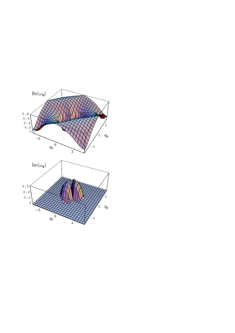
FIG. 9.: Real and imaginary parts of the spin-wave energy $\omega_{\bf q}$ ($U/t=10$ and $x=0.04$).

FIG. 10.: Spin-wave energy in the direction ${\bf q}=(q,q)$ for $U/t=10$ and $x=0.04$. Solid line: ${\rm Re}(\omega_{\bf q})$ (note the Goldstone mode at $q=Q\simeq 2.74$), dashed line: ${\rm Im}(\omega_{\bf q})$, dot-dashed line: excitation spectrum at half-filling [Eq. (100)]. The dotted lines indicate the boundaries of the particle-hole excitation spectrum.

FIG. 11.: Inverse propagators $\langle p_{\tilde{q}}p^{*}_{\tilde{q}}\rangle_{\omega=0}^{-1}$ (solid line) and $\langle q_{\tilde{q}}q^{*}_{\tilde{q}}\rangle_{\omega=0}^{-1}$ (dashed line) in the direction ${\bf q}=(q,q)$.

When $x\gg t^{2}/U^{2}$ (i.e. $x/p^{2}\ll 1$), it is tempting to neglect altogether the $x$ dependent terms in Eq. (99). This leads to

$$\omega_{\bf q}=\frac{J(1-p^{2})}{1-x}\Biggl{\{}\biggl{[}2+\frac{X^{2}_{\bf q}}{Y_{\bf q}-2}\biggr{]}^{2}-Y^{2}_{\bf q}\Biggr{\}}^{1/2},$$ (103)

which is the result obtained by Arrigoni and Strinati within an RPA analysis in the regime $t^{2}/U^{2}\ll x\ll 1$. [10] Although Eq. (103) reproduces the main features of the spin-wave-excitation spectrum (see Fig. 1 in Ref. [10]), it incorrectly predicts a vanishing of $\omega_{\bf q}$ along the line $q_{x}=q_{y}$. Even if there is no contradiction with Goldstone theorem, the approximation leading to Eq. (103) is too crude to yield a correct description of the Goldstone modes at $\pm{\bf Q}$.

D Spin-wave modes in the ferromagnetic phase

When $x\geq x_{c}$, the ground-state is ferromagnetic with $p=1$, i.e. ${\bf Q}=(2\pi,2\pi)\equiv(0,0)$. From Eqs. (95), (97) and (98), we obtain the spin-wave excitations

$$(1-x)\omega_{\bf q}=2t(x-x_{c})(2-Y_{\bf q})+xJ(2-Y_{\bf q})^{2}.$$ (104)

Since $Y_{{\bf q}=0}=2$, the mode at ${\bf q}=0$ is gapless, as expected for a ferromagnetic spin arrangement. For ${\bf q}\to 0$,

$$\omega_{\bf q}\simeq\frac{J_{\rm eff}}{2}q^{2},\,\,\,\,\,\,J_{\rm eff}=2t\frac{x-x_{c}}{1-x}.$$ (105)

The instability of the ferromagnetic phase against the formation of a spiral phase is signaled by a softening of the spin-wave modes, since the effective ferromagnetic exchange constant $J_{\rm eff}$ vanishes when $x\to x_{c}$. Note that for $x=x_{c}$, Eqs. (99) and (104) coincide and give $\omega_{\bf q}=xJ(2-Y_{\bf q})^{2}/(1-x)$.

IV Conclusion

In this paper, we have analyzed the semiclassical limit of the 2D Hubbard model in the framework of the spin-particle-hole coherent-state path integral. The main characteristic of the latter lies in the clear distinction between charge ($\gamma$) and spin (${\bf\Omega}$) degrees of freedom. The semiclassical analysis consists in expanding around a broken-symmetry ground-state by making a saddle-point approximation on the spin variables, while the fermionic degrees of freedom are integrated out within a systematic $t/U$ expansion. This should be contrasted with the Hartree-Fock/RPA theory whose validity in the strong-coupling limit is not obvious even at the semiclassical level. Nevertheless, we have shown that in the low-doping limit, the Hartree-Fock/RPA theory does recover the correct $t/U$ expansion. We have also justified the strong-coupling functional integral approach of Refs. [5, 6] where the electron-electron interaction is considered within a large-$U$ Hartree-Fock approximation while the SU(2) spin-rotation invariance is maintained by introducing a fluctuating spin-quantization axis. We expect however these approaches to break down with increasing doping since they do not capture all processes of order $t/U$. In the spin-particle-hole coherent-state path integral, a correct treatment of all processes of order $t/U$ follows from the consideration of the quartic term of the action $S[\gamma^{*},\gamma;{\bf\Omega}]$ [Eq. (5)].[29]

The spin-particle-hole coherent-state path integral provides a convenient framework for studying spin-wave modes around the semiclassical ground-state. In particular, it allows a systematic spin conserving analysis which ensures a proper description of the Goldstone modes of the system. From the mean-field fermionic self-energy, one can generate all vertex corrections to be taken into account in the propagator of the spin-wave modes. A mere calculation to order $O(t/U)$ of the effective action $S[p,q]$ of spin fluctuations would give a contradiction with Goldstone theorem. Given this observation, it is not surprising that a $t/U$ expansion of the RPA equations for the collective modes in the spiral phase meets with difficulties regarding a correct description of the Goldstone modes. [10]

Our main result is an analytical expression of the spin-wave excitations of the spiral phase over the entire Brillouin zone except in the vicinity of ${\bf q}=0$. Besides the gapless mode at ${\bf q}=0$, we find two Goldstone modes at $\pm{\bf Q}$ as expected for a spiral spin order. Our result agrees with previous numerical calculations and improves the analytical expression obtained in Ref. [10]. Although the spiral phase is unstable, as shown by a negative mean-field susceptibility and the presence of imaginary modes, we expect the short-wavelength fluctuation modes (with real energies) to survive in the actual ground-state of the system.

A Free energy in the mean-field state

In order to calculate the free energy $F$ [Eq. (25)], it is convenient to introduce a “Fermi wave vector” ${\bf K}_{F}(\alpha)=K_{F}(\alpha)(\cos\alpha,\sin\alpha)$ defined by $\epsilon_{{\bf K}_{F}(\alpha)}=0$. From Eq. (23), we deduce

$$K_{F}^{2}(\alpha)=2\frac{4tp-\mu}{\frac{\cos^{2}\alpha}{m_{x}}+\frac{\sin^{2}\alpha}{m_{y}}}.$$ (A1)

The free energy can be written as $F=N^{-1}\sum_{\bf k}(1-\theta(\epsilon_{\bf k}))\epsilon_{\bf k}$ where

$$\frac{1}{N}\sum_{\bf k}\epsilon_{\bf k} = -\mu-J(1-p^{2}),$$ (A2)

$$\frac{1}{N}\sum_{\bf k}\theta(\epsilon_{\bf k})\epsilon_{\bf k} = \frac{1}{N}\sum_{\bf K}\theta(\epsilon_{\bf K})\epsilon_{\bf K}$$ (A3)

$$\simeq \int_{0}^{2\pi}\frac{d\alpha}{2\pi}\int_{0}^{K_{F}(\alpha)}\frac{dK}{2\pi}K\Biggl{[}-\mu+4tp-\frac{K^{2}}{2}\Biggl{(}\frac{\cos^{2}\alpha}{m_{x}}+\frac{\sin^{2}\alpha}{m_{y}}\Biggr{)}\Biggr{]}$$ (A4)

$$= \frac{(4tp-\mu)^{2}}{4\pi}\sqrt{m_{x}m_{y}}.$$ (A5)

Eq. (25) follows from (A2) and (A5).

B Correction $F^{\prime}$ to the free energy

The contribution $F^{\prime}$ to the free energy (Fig. 5) is given by

$$F^{\prime}=\frac{1}{N^{2}\beta^{2}}\sum_{{\bf k},{\bf k}^{\prime}}\sum_{\omega,\omega^{\prime}}\Gamma^{\rm II}_{\uparrow\downarrow,\uparrow\downarrow}(i\omega,i\omega^{\prime};i\omega,i\omega^{\prime})[G^{(0)}_{\uparrow}(i\omega)]^{2}{\cal G}_{\uparrow}({\bf k},i\omega)(2tp\cos k_{\nu})^{2}[G^{(0)}_{\downarrow}(i\omega^{\prime})]^{2}{\cal G}_{\uparrow}({\bf k}^{\prime},i\omega^{\prime})\Bigl{(}2t\sin\frac{Q}{2}\sin k^{\prime}_{\nu}\Bigr{)}^{2}.$$ (B1)

Performing the sums over $\omega$ and $\omega^{\prime}$ and retaining the leading order term in $t/U$, we find (for $T\to 0$)

$$F^{\prime} = \frac{1}{UN^{2}}\sum_{{\bf k},{\bf k}^{\prime}}\theta(\epsilon_{\bf k})(1-\theta(\epsilon_{{\bf k}^{\prime}}))(2tp\cos k_{\nu})^{2}\Bigl{(}2t\sin\frac{Q}{2}\sin k^{\prime}_{\nu}\Bigr{)}^{2}\frac{1}{(\epsilon_{\bf k}+\mu)^{2}}.$$ (B2)

Using

$$\frac{1}{N}\sum_{\bf k}\theta(\epsilon_{\bf k})4t^{2}p^{2}\frac{(\cos k_{\nu})^{2}}{(\epsilon_{\bf k}+\mu)^{2}}\simeq\frac{1}{N}\sum_{\bf k}\theta(\epsilon_{\bf k})\frac{(4tp)^{2}}{(\epsilon_{{\bf k}=0}+\mu)^{2}}=x$$ (B3)

we obtain $F^{\prime}=xJ(1-p^{2})$ in the limit $x\ll 1$.

REFERENCES

- [1] H.J. Schulz, Phys. Rev. Lett. 65, 2462 (1990).
- [2] A. Singh, Z. Tešanović and J.H. Kim, Phys. Rev. B 44, 7757 (1991).
- [3] E. Arrigoni and G.C. Strinati, Phys. Rev. B 44, 7455 (1991).
- [4] M. Dzierzawa, Z. Phys. B 86, 49 (1992).
- [5] C. Zhou and H.J. Schulz, Phys. Rev. B (1995).
- [6] C. Zhou, Ph.D thesis, Université d’Orsay, 1994 (unpublished).
- [7] A.V. Chubukov and K.A. Musaelian, Phys. Rev. B 51, 12605 (1995).
- [8] W. Brenig, Ann. Physik 5, 123 (1996).
- [9] A.P. Kampf, Phys. Rev. B 53, 747 (1996).
- [10] Arrigoni and Strinati, Eur. Phys. J. B 19, 433 (2001).
- [11] R. Frésard, M. Dzierzawa and P. Wölfle, Europhys. Lett. 15, 325 (1991); R. Frésard and P. Wölfle, J. Phys.: Condens. Matter 4, 3625 (1992).
- [12] C. Jayaprakash, H.R. Krishnamurthy and S. Sarker, Phys. Rev. B 40, 2610 (1989).
- [13] D. Yoshioka, J. Phys. Soc. Japan 58, 1516 (1989).
- [14] C.L. Kane, P.A. Lee, T.K. Ng, B. Chakraborty and N. Read, Phys. Rev. B 41, 2653 (1990).
- [15] A. Auerbach and D.E. Larson, Phys. Rev. B 43, 7800 (1991).
- [16] J. Gan, N. Andrei and P. Coleman, J. Phys.: Condens. Matter 3, 3537 (1991).
- [17] B.L. Schraiman and E.D. Siggia, Phys. Rev. Lett. 62, 1564 (1989); Phys. Rev. B 46, 8305 (1992).
- [18] T. Dombre, J. Phys. (France) 51, 847 (1989).
- [19] J.R. Schrieffer, X.G. Wen and S.C. Zhang, Phys. Rev. B 61, 2814 (1988).
- [20] A. Singh and Z. Tešanović, Phys. Rev. B 41, 614 (1990).
- [21] A. Auerbach and B.E. Larson, Phys. Rev. Lett. 66, 2262 (1991).
- [22] See M.A. Kastner and R.J. Birgeneau, Rev. Mod. Phys. 70, 897 (1998), and references therein.
- [23] N. Dupuis and S. Pairault, Int. J. Mod. Phys. B 14, 2529 (2000).
- [24] N. Dupuis, preprint cond-mat/0105xxx.
- [25] Alternatively, Eq. (26) can be obtained from .
- [26] More precisely, we find for , and for .
- [27] A. Auerbach, Interacting Electrons and Quantum Magnetism (Springer Verlag, New York, 1994).
- [28] E. Rastelli, L. Reatto and A. Tassi, J. Phys. C: Solid State Phys. 18, 353 (1985).
- [29] By integrating out the UHB in the partition function [see Eq. (5)], one recovers the action of the - model in the spin-hole coherent state path integral. [23] The two-particle atomic vertex plays a crucial role in this derivation whatever the value of the doping. At half-filling, the action of the Heisenberg can be obtained in a more direct way by integrating out all fermionic degrees of freedom at once. In that case does not enter the derivation. The role of is therefore dependent on the way charge or spin degrees of freedom are integrated out.