[
Magnetic phase separation in ordered alloys
Abstract
We present a lattice model to study the equilibrium phase diagram of ordered alloys with one magnetic component that exhibits a low temperature phase separation between paramagnetic and ferromagnetic phases. The model is constructed from the experimental facts observed in Cu3-xAlMnx and it includes coupling between configurational and magnetic degrees of freedom which are appropriated for reproducing the low temperature miscibility gap. The essential ingredient for the occurrence of such a coexistence region is the development of ferromagnetic order induced by the long-range atomic order of the magnetic component. A comparative study of both mean-field and Monte Carlo solutions is presented. Moreover, the model may enable the study of the structure of the ferromagnetic domains embedded in the non-magnetic matrix. This is relevant in relation to phenomena such as magnetoresistance and paramagnetism.
pacs:
PACS number: 75.40.Mg, 64.60.Cn, 64.75.+g]
I Introduction
Recently, renewed interest has been addressed to ferromagnetic ordered alloys. This is because of the unique properties arising from the interplay between elasticity, magnetism and (configurational) atomic order. From the point of view of applications, the development of new actuator materials having very large magnetostrains [1] is particularly interesting . Also relevant is the possibility of having superparamagnetism [2] and giant magnetoresistance [3] both associated with coexistence of magnetic domains (large magnetic particles) embedded in a non-magnetic matrix. This mixed phase has been observed, for instance, in the Cu3-xAlMnx Heusler alloy.
The Heusler alloys are ternary intermetallic compounds with the composition X2YZ and a low temperature structure. At high temperatures the stable phase corresponds to a disordered bcc lattice, also called phase, and undergoes a two-stage disorder-order transition , as the temperature is decreased. Especially interesting are the Mn-based Heusler alloys [4, 5, 6, 7], which exhibit a magnetic moment approximately located on the Mn atoms [8]. Among them, the most extensively studied are the Ni2GaMn [9, 10] and the Cu2AlMn [11, 12, 13, 14, 15, 16, 17] alloys. In both cases, the phase is ferromagnetic but the phase is paramagnetic. This close relation between atomic order and magnetic properties has been known to scientists for many years [18]. Additionally, these alloys exhibit shape-memory effects, intimately related to the structural transition, of the martensitic type [19], undergone at low temperatures. It has been suggested that the control of shape-memory properties by application of an external magnetic field is a principle for operation of the new class of actuator materials [20, 21]
In Cu-Al-Mn the martensitic transition only exists [14] for compositions which are very far from the stoichiometry (Cu2AlMn) where the ordered phase is paramagnetic [22]. Nevertheless, the influence of magnetism coming from Mn is revealed in several experiments [23]. As well as the phase transitions mentioned above, the system exhibits, at low temperatures, a spinodal decomposition along the line Cu3Al - Cu2AlMn [11, 12, 24]. We will centre our attention on this two-phase region and denote the Cu-rich portion of the phase diagram of interest in this paper by Cu3-xAlMnx, with , . In Figure 1 we show schematically the corresponding phase diagram as it is obtained from experiment. The continuous lines are drawn from the data in Ref. [24], whereas the points at and are from Refs. [25] and [26] respectively.
The low temperature ordered structures for the limiting values of are different. The Cu3Al binary alloy is at low temperatures, [27] whereas the Cu2AlMn is and ferromagnetic, with a relatively high Curie temperature ( K) [28]. The ferromagnetism of the phase appears as a consequence of the atomic ordering of the Mn atoms. In this sense it is known that properties such as the saturation magnetic moment depends on the degree of order of the Mn atoms [29]. It then naturally follows that the absence of magnetism (long-range magnetic order) either in the high temperature -phase or in the low temperature phase ( or ), for small values of , might well be related to the tendency for the Mn atoms to distribute themselves randomly at the different lattice sites. On the other hand, by increasing the amount of Mn, for instance in the Cu3AlMn2 alloy, the resulting magnetic interaction is antiferromagnetic [29]. Such different magnetic behaviour may be understood in terms of the oscillatory RKKY interaction between the magnetic moments of the Mn atoms [30, 17, 31].
The phase separation or miscibility gap in Cu2AlMn occurs at temperatures below K [12] (see Figure 1) and gives rise to a coexistence region between a non-magnetic phase and a ferromagnetic phase, with low and high Mn content respectively. The occurrence of superparamagnetism [2] or magnetoresistance [3] are both directly related to the existence of magnetic clusters ( stable domains) immersed in the non-magnetic () matrix. Some aspects of this phase diagram are not totally clear. Firstly, the persistence of a stable phase for small values of . Kainuma et al.[24], by using X-ray diffraction measurements, have detected an abrupt change in the intensity of the superstructure peaks at . It should be mentioned that this effect was not found in other earlier studies [11]. Other important information, not yet available, refers to the different atomic distributions for the non-stoichiometric structure. Some assumptions on this matter will be required in order to perform a theoretical study. Other aspects that need to be discussed refer to the characteristics of the coexisting phases. They will depend on the location of the - (according to the results in Ref. [24]) and magnetic transition lines with respect to the coexistence line. More precisely, depending on the temperatures at which such interphases end on the coexistence line, the phases may be different in atomic order (,) or/and magnetic order (ferromagnetic, paramagnetic). In this sense, even the coexistence of two different paramagnetic and phases (upper part of the miscibility gap in Figure 1), with a very similar content of Mn, are suggested [24].
In this paper we present a lattice model able to reproduce the main features of the equilibrium phase diagram in this two-phase region. The details of the model will be derived from a microscopic description of the atomic and magnetic properties of Cu3-xAlMnx alloys. Nevertheless, it can be applied to other systems. Practical reasons will require several hypotheses which in some cases are not totally justified a priori but only later from agreement of obtained results with experimental data. This agreement is indicative that the model captures the essential physics and provides a starting point for future more exhaustive studies. The model is a projection of the ternary alloy onto a binary system, when one of the species is magnetic. It is constructed on the basis that the main physics of the phenomena lies on the atomic ordering of the magnetic component which moreover is taken to be always the less abundant. The effective Hamiltonian accounts for a purely configurational ordering energy between first neighbouring pairs so that at low temperatures the magnetic atoms tend to be second neighbours. Then a simple ferromagnetic pair interaction between next-nearest neighbours is enough to give rise to a low temperature phase separation between a non-magnetic phase and a ferromagnetic phase that, moreover, may have different ordered structures.
It has been suggested [24] that the occurrence of the two-phase region in Cu3-xAlMnx cannot be attributed to either chemical(configurational) or magnetic ordering. In this work, we use a very simple microscopic model to show that the coupling between both atomic (configurational) and magnetic orderings is sufficient to give rise to a decomposition between two phases at low temperatures. This coupling operates in such a way that as the atomic ordering develops the (indirect) exchange interactions between the atomic moments of the magnetic particles produce a long-range ferromagnetic order.
The remainder of the paper is organized as follows. In section II we introduce the model. Section III is devoted to its mean-field solution. In order to better understand the nature of the different phases and the behaviour of several measurable quantities we also solve the model by using Monte Carlo numerical simulations. This is presented in section IV. Finally in section V we summarize and conclude.
II Model
In the present study, our main goal is to understand the formation of the miscibility gap in Cu3-xAlMnx along the line . The complexity inherent to the description of a magnetic ternary alloy has led us to make simplifications that we shall discuss in this section. Indeed, the quest for reasonable simplifications becomes compulsory in order to perform the Monte Carlo numerical simulations. Although the inclusion of too many ingredients (and thus free parameters) in the model may lead to a better fit of the available data (in our case scarce), it may hide the understanding of the relevant physical mechanism underlying the phase diagram properties, which we believe is the coupling between the long-range configurational (chemical) ordering and the magnetism of the Mn atoms.
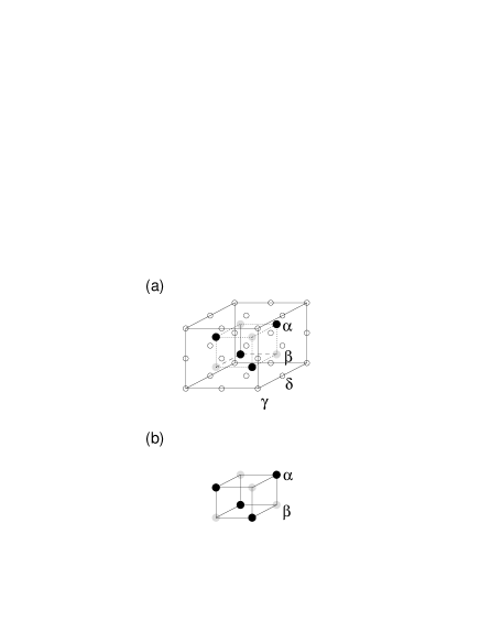
The equilibrium structure of Cu3-xAlMnx can be described as an underlying structure formed by the superposition of four interpenetrated sublattices, named , , and (see Figure 2a). In order to describe the different phases of the system it is convenient to specify the occupation probabilities of the different species X (=Cu,Al,Mn) in the four different sublattices (=, , , ). Tables I and II summarize the occupation probabilities for the limiting () and () stoichiometric phases. For intermediate values of a more elaborate discussion is required.
We start with the region corresponding to small values of , . Recently [24], X-ray diffraction experiments shown that the structure persists above the coexistence region for values of up to . In other words, the addition of a small amount of Mn does not break the symmetry ==. This is an (a priori) unexpected result, given the different atomic environments of these sublattices in the phase. In any case, it seems clear that entropy plays a very important role in the stability of this homogeneous phase. From Figure 1 it follows that for the stability is extended to higher temperatures as the value of increases. A natural hypothesis is, therefore, to assume that (for low values of ) the Mn atoms behave as impurities that are randomly distributed on the four different sublattices. The corresponding occupation probabilities are indicated in Table III.
In the region the stable phase is of the type. There are several atomic distributions that are compatible with the symmetry = . Table IV displays the occupation probabilities in the most straightforward case for which the Mn concentrates in a unique sublattice. Alternatively, in a more general way, one might write the occupation probabilities (Table V) in terms of a free parameter (). Notice that these atomic distributions account for a continuous change from the phase () to the phase ().
The next step is to introduce the two major simplifications of the model:
-
1.
The structures described in tables I to V have the existence of two n.n. sublattices ( and ) in common which contain most of the Cu atoms and have identical occupation probabilities: . Experimentally, this symmetry with respect to the and sublattices seems to be satisfied for any concentration and temperature ranges. From now on we forget about them and concentrate on the atomic distribution behaviour on the other two remaining sublattices, motivated by the feeling that the breaking down of the - symmetry is crucial in the ordering of the Mn atoms at low temperatures. This, of course, will restrict the validity of our study to temperatures below the - transition, which is precisely the region of interest here. Therefore, the model will be defined on a simple cubic lattice divided into two sublattices, and , as illustrated in Figure 2b.
-
2.
Continuing with our assumption that the main physics lies on the atomic ordering of the Mn atoms, we shall proceed further by distinguishing between magnetic and non-magnetic atoms only. In our binary alloy model, , the non-magnetic species stands either for Cu or Al, whereas the magnetic species stands for Mn and the composition is restricted to . The behaviour of the atoms on sublattices and can be regarded as a simple order-disorder transition. For small values of both sublattices are equally populated by B-atoms (behaving as impurities) while for larger values of , B atoms occupy preferably one of the two sublattices. Moreover, this behaviour depends on temperature. As regards the configurational ordering, the model gives rise to two phases only: disordered and ordered, corresponding to low () and high () content of the magnetic species respectively. Keeping this correspondence in mind, in what follows we shall use the simplified notation D (disordered) and O (ordered).
We notice that the quantitative study of properties such as the magnetization, susceptibility or other properties related to magnetism (magnetoresistance, etc..) is not our goal here. Rather, we shall focus on how the development of long-range ferromagnetic order (resulting from the interplay with the atomic order) determines the phase diagram at low temperatures as a function of the content of the magnetic species . In what the model description concerns, this can be achieved by considering localized Ising-like spin variables associated with each atom.
We start from the following pair-interaction effective Hamiltonian:
| (1) | |||||
| (2) | |||||
| (3) |
where and are the configurational and magnetic energy contributions respectively. The summation is performed over the different -nearest-neighbour shells (up to ), is the number of -th nearest-neighbour - pairs and are their corresponding pair-interaction energy. Note that the magnetic contribution only involves atoms. We have indicated by and the two possible magnetic states. To preserve the symmetry under exchange of the and magnetic states we take .
Following standard procedures, we write Hamiltonian (1) in terms of Ising-like variables defined at each lattice site. Let us index the sites of the cubic lattice by (). At each lattice site we define the following two coupled two-state variables and . The variable represents the non-magnetic and magnetic species ( and ) respectively, then, provided , we define describing the two possible magnetic states of each atom.
Considering interactions up to next-nearest neighbours (), the configurational energy term in equation (1) can be written, neglecting constant terms, as:
| (4) |
where the first two summations are extended to nearest neighbour(n.n.) and next-nearest neighbours (n.n.n.) respectively, and the Hamiltonian parameters are:
| (5) |
| (6) |
and
| (7) |
where and are the number of n.n. and n.n.n. of each lattice site respectively. In the Canonical ensemble, the last term in equation (4) is just a simple energy shift which depends on the alloy concentration. As regards the magnetic energy term it can be rewritten as:
| (11) | |||||
where:
| (12) |
| (13) |
We notice that the latter two terms in equation (11) do not depend on the magnetic variables . Expanding the different contributions in (11) and ignoring constant terms, the Hamiltonian becomes:
| (14) | |||||
| (15) | |||||
| (16) |
The superscripts in the model parameters denote its configurational (c) or magnetic (m) origin, whereas the subscripts mean first- (1) or second- (2) neighbour interactions. In order to reduce the number of free model parameters we set . Indeed, the n.n magnetic interaction between pairs is not essential for our present purposes since we restrict ourselves to the case in which the ferromagnetism develops in the configurationally ordered phase. Furthermore, by using reduced energy units , we get the following minimal model Hamiltonian:
| (17) | |||||
| (18) |
where the parameters are:
| (19) |
which measures the ordering energy between second-neighbour pairs either , and , independently of the magnetic state of atom , and
| (20) |
which accounts for the ferromagnetic interaction between second-neighbour pairs.
III Mean Field solution
This section is devoted to the solution of the model introduced previously for the A1-cBc binary alloy by using standard mean-field techniques based on the Bragg-Williams approximation. We denote the occupation numbers for each component () in each sublattice () by and consider the following order parameters:
| (21) |
| (22) |
| (23) |
where () is the molar fraction of the magnetic species, () is the atomic order parameter and () measures the magnetization of the system. Using standard procedures, in the Grand Canonical formulation, we obtain the following expression for the internal energy:
| (25) | |||||
where and is the chemical potential difference between the two species. The corresponding entropy is given by:
| (26) |
Expressions (25) and (26) produce the following free energy:
| (27) | |||||
| (28) | |||||
| (29) | |||||
| (30) | |||||
| (31) | |||||
| (32) | |||||
| (33) | |||||
| (34) |
with and . The free energy in (27), in the absence of magnetism, reduces to the standard case of order-disorder, but one of the species is twice degenerate. When magnetism is taken into account, model (27) exhibits two phase transitions respectively associated with the order parameters and . We denote the respective transition temperatures by and . Since we are interested in the case of , the model parameters must be taken so that .
The equilibrium temperature dependence of the order parameters was obtained from direct minimization of the function (27). In figure 3 we show the section of the phase diagram for different values of and and . Three different phases may appear. The Disordered-Paramagnetic (DP) phase with and , the Ordered-Paramagnetic (OP) phase with and and the Ordered-Ferromagnetic (OF) phase with and . Both parameters and have the effect of increasing the stability of the ordered (OP and OF) phases. Continuous lines stand for second-order phase transitions, whereas the dashed ones stand for discontinuous phase transitions. The intersection between the three interphases corresponds to a bicritical point in cases (a) and (b), whereas for (c) and (d) it corresponds to a triple point. The DP-OF transition is always first order, whereas the other two OP-OF and DP-OP may be second or first order. When the transition is first order, a phase separation shows up in the section. This is illustrated in Figure 4 for cases (b) and (c) corresponding to the previous picture (Figure 3).
In both cases of Figure 4 a phase separation between a non-magnetic (paramagnetic) and a ferromagnetic phases exists. At low temperatures the coexisting phases (DP+OF) are also different in their atomic ordered structure, whereas at moderate temperatures (OP+OF) both exhibit the same atomic structure. Besides, for case (b) (a larger value of ) a phase separation (DP+OP) between two non-magnetic phases appears. In this case, there exists a line of triple points (horizontal dot-dashed line). In Figure 5 we show the corresponding temperature behaviour of the order parameters and for different values of the composition . This information is obtained from the calculations presented in Figure 4 taking into account the fact that in the phase separation region the system is heterogeneous and that at constant concentration both the characteristics and the amount of the coexisting phases change with temperature. It is noticeable that in both cases the two order parameters ( and ) exhibit an anomaly at a given temperature, (a) and (b) . These temperatures correspond to the bicritical and the triple point discussed in Figure 3. When crossing the triple point line (case (b)), the anomaly is accompanied by a discontinuity in the order parameters.
IV Monte Carlo simulation
Monte Carlo simulations of model (17) have been performed in order to study the role of fluctuations. Starting from an initial (arbitrary) configuration, the subsequent microscopic configurations are generated by using the standard Metropolis algorithm. We have focussed on two cases. First, on the stoichiometric alloy () for different values of the parameters and . Secondly, we have fixed and and have studied the phase diagram as a function of and .
A Simulation details
The main results were obtained on a simple cubic lattice of size (). Moreover, a certain number of simulations with and were also carried out in order to study finite-size effects and to obtain illustrative real space snapshots of the system. Energy and order parameter fluctuations are measured according to the following definitions:
| (35) |
| (36) |
| (37) |
The brackets stand for Monte Carlo (MC) averages, performed over a large number of uncorrelated configurations after the equilibration of the system. In order to find the phase diagram, the transition lines were located from the positions of the peaks of the above quantities. In many cases equilibration was checked by testing the fluctuation-dissipation theorem, i.e.:
| (38) |
Two kinds of numerical simulation experiments have been performed:
-
1.
Grand Canonical simulations. The simulations in the Grand Canonical Ensemble have the advantage of allowing faster equilibration. The alloy concentration is not fixed and an additional term taking into account the effect of the chemical potential difference between both species is needed in this case. Formally, this is done by a Legendre transformation of the Hamiltonian (17). This yields:
(39) (40) Starting from an (arbitrary) initial configuration, the system at constant and , evolves towards equilibrium by means of Glauber excitations proposed in both variables, and independently. The unit of time MCS (a Monte Carlo step) is defined as independent proposals of each kind of flip on a randomly selected lattice site. Typically the averages are performed over configurations, taken every MCS and discarding the initial MCS for equilibration. The regions of phase separation correspond to unreachable regions in the phase diagram.
-
2.
Canonical simulations. In these simulations the Glauber excitations are proposed in the magnetic variable only. In order to preserve the alloy composition , the variables evolve according to the Kawasaki exchange dynamics. The equilibration process is much slower in this case and the system may get trapped in metastable configurations. To get rid of such configurations, it is convenient to allow a certain fraction () of exchanges between n.n.n. atoms. Then, a MCS is in this case defined as proposals of flips, proposals of n.n. exchanges and proposals of n.n.n. exchanges. We have studied the effect of different values of and found that is enough to reach equilibrium in a reasonable time. Typically averages are performed over configurations, taken every MCS, after discarding the first MCS for equilibration. In the region of phase separation the simulated system evolves to an inhomogeneous “slab” configuration with a flat interface. Because of finite-size effects, the energy of such configurations is very much dominated by the interfacial energy and should be carefully analyzed. In spite of the long times needed to get reliable results, the simulations in the Canonical ensemble are very useful here since they provide information concerning the structure of the domains in the coexistence region.
B Monte Carlo Results
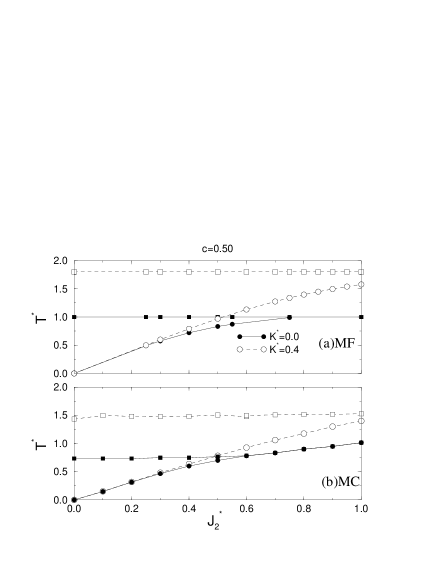
We start by presenting the transition temperatures as a function of the model parameters for the case of the stoichiometric alloy . This is shown in the lower part of Figure 6 (b). A comparative look of both mean-field (a) and MC results (b) reveals that both solutions render the same qualitative behaviour. The fluctuations (taken into account in the Monte Carlo solution) have the effect of increasing the stability of the disordered, paramagnetic phases so that the overall transition temperatures are lower than in the mean-field solution.
Figure 7 shows the section of the phase diagram, drawn from the Grand Canonical simulations, with , and . We notice that the model parameters are those of Fig. 3(d). It follows that both numerical simulations and mean-field techniques render the same qualitative phase diagram. The only remark that comes out is the smearing out of the re-entrant (OP) phase in the MC solution, due to the fluctuations. The available MC data does not allow for a conclusive determination of the nature (first or second-order) of the transitions.
In order to compare data with experiment, the study of the section of the phase diagram is essential. It turns out to be a tough task because of the finite-size effects. In particular, to definitively resolve the coexistence region, one needs to use very large linear system sizes.
Figure 8 shows the phase diagram corresponding to and . In Fig. 8a we simultaneously show the mean-field and the MC solutions. One observes that the main trends of both phase diagrams are the same. For practical reasons, we show the MC solution in more detail in Fig. 8b . The phase transition lines and the limits of the coexistence region, have been located from the peaks observed in the specific heat . This criterion has been followed in both the Grand Canonical (open diamonds) and Canonical (black diamonds) simulations . In the Grand Canonical simulations the coexistence region is revealed by unreachable zones in the diagram accompanied by flat steps in the curves of constant (three examples are depicted by small dots joined by a thin line).
When comparing the results corresponding to the same system size obtained from both the Canonical and the Grand Canonical simulations we see that in the former the coexistence line occurs at lower temperatures. This is due to finite-size effects that have a strong influence on the stabilization of the mixed phase configurations. In this sense we have checked that when the system size is increased this effect is corrected and the phase separation occurs at higher temperatures. To illustrate this, we have plotted in Figure 8 (with thick dashed lines) the upper part of the coexistence line obtained from Canonical simulations, for two different values of the system size (= 16 and =24), as indicated.
The same effect appears when studying the specific heat. In Figure 9 we show the temperature behaviour of the specific heat (a) together with the order parameters and (b) for , and as obtained from the canonical MC simulations. Data shown correspond to and . Note that the peak corresponding to the phase separation shows a much larger dependence on than the peak corresponding to the order-disorder transition. The inset (c) shows the specific heat computed from the energy fluctuations (equation 35) and from the derivative of the average energy (equation 38). The agreement ensures that the equilibration times considered are long enough.
In spite of the difficulties described above, which certainly hinder the location of the boundaries, the phase diagram presented in Figure 8 is essentially similar to that obtained experimentally (see Figure 1) at least at moderate and low temperatures. The lack of resolution in the results makes it impossible to conclude whether or not the MC results render a line of triple points as occurs in the mean-field solution (lower part of 4). Unfortunately, the existing experimental data do not provide new information on this point. We suggest that more experiments are needed. Provided that the experimental phase diagram is sufficiently well resolved, fine tuning of the parameters and (even ) would allow the matching of more details.
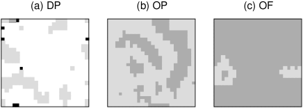
Besides the determination of the phase diagram and the fluctuations, the MC simulations have the possibility of providing real space snapshots of the system configuration. Figure 10 shows a two dimensional section of the simulated system with for different homogeneous equilibrium phases corresponding to the phase diagram in Figure 8. Case (a) corresponds to the DP phase with and , (b) to the OP phase with and and (c) to the OF phase with and . The assignment of the different colours has been done by measuring the short-range order parameters in a cell of size centered at each lattice site of a certain two-dimensional horizontal cut of the original system. When the values of the local magnetization and/or local order parameter are above the corresponding lattice site is considered to belong to a ferromagnetic and/or to an atomically ordered phase respectively. White, light gray and dark gray indicate DP, OP and OF regions. Black corresponds to local disordered ferromagnetic regions which do not correspond to any stable phase. These appear because the fluctuations become both more probable and important with temperature in the homogeneous phases. Actually, the three snapshots correspond to a time evolution of MCS, when the average values of the long-range order parameters are perfectly equilibrated. Thus, the curved interfaces reveal that the fluctuations evolve with time and appear and disappear very quickly.
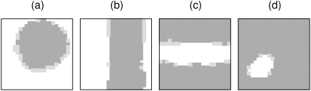
In Figure 11 we show snapshots of the system configuration inside the coexistence region. The four pictures correspond to and to different values of the composition; (a) , (b) , (c) and (d) . Note that for low concentration of the magnetic component (a), the OF phase consists of ferromagnetic bubbles inside the DP matrix as expected. For larger values of the ferromagnetic bubbles transform into rods or slabs (b). This is an artifact of finite-size effects that makes the system decrease the interfacial energy by taking advantage of the periodic boundary conditions. Cases (c) and (d) are symmetric to (b) and (a) respectively. Given the large value of , the matrix is ferromagnetic and the domains paramagnetic.
It is known that the shape and the size of the magnetic bubbles embedded into the non-magnetic matrix is crucial for the occurrence of magnetoresistance. In the light of the present results, we believe the present model is suitable for determining the optimum characteristics of such domains. Along these lines, the study of the kinetics of the domain growth after quenches from high temperature should supply useful information. This will be the subject of future work.
V Conclusion
By using a simple lattice model we have shown that the magnetism of an ordered alloy may give rise to a low temperature phase separation between a ferromagnetic phase and a paramagnetic phase. The existence of this mixed phase is relevant in relation to the occurrence of phenomena such as paramagnetism and magnetoresistance.
This study has been motivated by the behaviour observed in Cu3-xAlMnx. Nevertheless, the strategy followed in the construction of the model should apply to other alloys. In particular, to those in which the ferromagnetism is induced by the configurational ordering of the magnetic atoms, as occurs in Cu3-xAlMnx. Our main conclusion is that this interplay between both kind of orderings is enough to produce the magnetic phase separation. We should mention that other effects such as elasticity due to the different atomic size of the elements may affect the final phase diagram. In spite of this and in view of the present results it is clear that the model captures the essential ingredients and makes it an appropriate starting point for future dynamical studies of the kinetics of formation of the mixed phase after a suitable thermal quench.
Acknowledgements
We acknowledge fruitful discussions with Antoni Planes. The authors also acknowledge financial support from CICyT project number MAT98-0315. J.M. acknowledges financial support from Direcció General de Recerca (Catalonia).
REFERENCES
- [1] K.Ullakko, P.T.Jakovenko and V.G.Gavriljuk, in Proccedings of Smart Structures and Materials, ed. V.V.Varadan and J.Chandra, Vol. 2715, pp. 42-50, SPIE, San Diego, USA, 1996.
- [2] T.V.Yefimova, V.V.Kokorin, V.V.PolotnyuK and A.D.Shevchenko, Phys. Met. Metallogr. 64, 189 (1987).
- [3] L.Yiping, A.Murthy, G.C.Hadjipanayis and H.Wan, Phys. Rev. B 54, 3033 (1996).
- [4] P.J.Webster, Contemp. Phys. 10, 559 (1969).
- [5] P.J.Webster, K.R.A.Ziebeck, S.L.Town and M.S.Peak, Phil. Mag. B 49, 295 (1984).
- [6] J.S.Robinson, S.J.Kennedy and R.Street, J.Phys.:Condens. Matter. 9, 1877 (1997).
- [7] S.Plogmann, T.Schlathölter, J.Braun, M.Neumann, Yu.M.Yarmonshenko, M.V.Yablonskikh, E.I.Shreder, E.Z.Kurmaev, A.Wrona and A.Slebarski, Phys. Rev. B 60, 6428 (1999).
- [8] Y.Ishikawa, Physica B 91, 130 (1977).
- [9] A.Planes, E.Obradó, A.Gonzàlez-Comas and Ll.Mañosa, Phys. Rev. Lett. 79, 3926 (1997) and references therein.
- [10] T.Castán, E.Vives and P.-A.Lindgård, Phys. Rev. B 60, 7071 (1999) and references therein.
- [11] J.Soltys, Phys. Stat. Solidi A 63, 401 (1981).
- [12] M.Bouchrad, G.Thomas, Acta Metall. 23, 1485 (1975).
- [13] M.Prado, F.Sade and F.Lovey, Scr. Metall. Mater. 28, 545 (1993).
- [14] E.Obrado, Ll.Mañosa and A.Planes, Phys. Rev. B 56, 20 (1997).
- [15] E.Obrado, C.Frontera, Ll.Mañosa and A.Planes, Phys. Rev. B 58, 14245 (1998).
- [16] E.Obrado, A.Planes, B.Martinez, Phys. Rev. B 59, 11450 (1999).
- [17] E.Obrado, E.Vives and A.Planes, Phys. Rev. B 59, 13901 (1999).
- [18] A.J.Bradley and J.W.Rodgers, Proc. Soc. London, A 144, 340 (1934).
- [19] L.Delaey, in Materials Science and Technology, edited by P.Haasen (VCH, Weinheim, 1991), Vol. 5, p.339.
- [20] K.Ullakko, J.K.Huang, C.Kantner, R.C.O’Handley and V.V.Kokorin, Appl. Phys. Lett. 69, 1966 (1996).
- [21] A.A.Likhachev, K.Ullakko, preprint 1999.
- [22] In the case of , the cubic phase which transforms martensitically is ferromagnetic.
- [23] J.Marcos, A.Planes, Ll.Mañosa, A.Labarta and B.J.Hattink, Preprint.
- [24] R.Kainuma, N.Satoh, X.J.Liu, I.Ohnuma and K.Ishida, J. Alloys Comp. 266. 191 (1998).
- [25] E.Obradó, PhD. Thesis, Universitat de Barcelona 1999.
- [26] K.Nicolaus, PhD. Thesis, Technische Universität München 2000.
- [27] J.L.Murray, in Binary alloy phase diagrams, ed. T.B.Massalski (American Society for Metals, Ohio, 1986), Vol. 1, p. 103.
- [28] D.R.F.West, D.Lloyd Thomas, J.Ins. Met. 85, 97 (1956).
- [29] G.B.Johnston, E.O.Hall, J.Phys. Chem. Solids 29, 201 (1968).
- [30] K.Tajima, Y.Ishikawa, P.J.Webster, M.W.Stringfellow, D.Tochetti and K.R.A.Ziebeck, J. Phys. Soc. Jpn. 43, 483 (1977).
- [31] E.Vives, E.Obradó and A.Planes, Physica B 275, 45 (2000).