Ballistic spin-polarized transport and Rashba spin precession in semiconductor nanowires

Abstract

We present numerical calculations of the ballistic spin-transport properties of quasi-one-dimensional wires in the presence of the spin-orbit (Rashba) interaction. A tight-binding analog of the Rashba Hamiltonian which models the Rashba effect is used. By varying the robustness of the Rashba coupling and the width of the wire, weak and strong coupling regimes are identified. Perfect electron spin-modulation is found for the former regime, regardless of the incident Fermi energy and mode number. In the latter however, the spin-conductance has a strong energy dependence due to a nontrivial subband intermixing induced by the strong Rashba coupling. This would imply a strong suppression of the spin-modulation at higher temperatures and source-drain voltages. The results may be of relevance for the implementation of quasi-one-dimensional spin transistor devices.

PACS numbers: 72.25.Dc, 73.23.Ad, 73.63.Nm

I INTRODUCTION

The electron spin precession phenomena at zero magnetic field induced by a variable spin-orbit interaction in quasi-two-dimensional electron gas (2DEG) systems, was first elucidated by Datta and Das[1] as the basic principle for the realization of a novel electronic device, the spin-transistor. The underlying idea is to drive a modulated spin-polarized current (spin-inject and detect) entirely electrically, combining just ferromagnetic metals and semiconductor materials. For this, the spin-precession is controlled via the spin-orbit coupling (Rashba-coupling[2, 3]) associated with the interfacial electric fields present in the quantum well that contains the 2DEG channel. The tuning of the Rashba coupling by an external gate voltage, was recently demonstrated in different semiconductors by Nitta et al.[4] and others[5, 6, 7], and more recently by Grundler[8] applying a back gate voltage while the carrier density was kept constant. It has been also achieved in a p-type InAs semiconductor by Matsuyama et al.[9]

Although spin injection has already been reported from ferromagnetic metals to InAs based semiconductors, [10, 11] the spin polarization signatures reported are about 1% or less, making the results very controversial. Such low efficiency can be also attributed to extraneous effects, such as the local Hall effect,[12, 13] and to resistance mismatch at the interfaces between the ferromagnetic metal and the semiconductor.[14] Very recently, one of us has proposed that the latter problem can be circumvented by growing atomically ordered and appropriately oriented interfaces of ferromagnetic metals and suitable semiconductors, that act as perfect spin-filters and make injection of up to $100\%$ spin-polarized electrons into semiconductors possible in principle. [15] If this prediction is confirmed experimentally, a major obstacle to the spin injection experiments will be overcome.

On the other hand, another crucial prerequisite to having an overall strong spin current modulation, is to restrict the angular distribution of electrons in the 2DEG by imposing a strong enough, transverse confining potential.[1] This was the original proposal of Datta and Das. It was argued that if $W$ is the width of the transverse confining potential well, the condition $W\ll\hbar^{2}/\alpha m^{*}$, should be satisfied for the intersubband mixing to be negligible, which would ensure a perfect spin-current modulation. If we choose a typical channel in an In_0.53Ga_0.47As semiconductor, with $m^{*}=0.042\,m_{o}$, and spin-orbit coupling constant $\alpha=1.5\times 10^{-11}$ eV m, [6] this implies $W\ll 0.38\mu$m. This width is of the order or much smaller than the characteristics lateral widths of the 2DEG channels patterned in the current experimental studies of spin-injection.[10, 11, 12] This would suggest that in order to achieve better results in the spin-injection modulation, the best choice would be ballistic quasi-one dimensional systems (by introducing split gates for instance), where just a few populated subbands are allowed, rather than the quasi-two-dimensional situation, in which many propagation channels exist (Hall-bar experiments), with a concomitant small subband spacing comparable to the zero field spin-splitting energy of the 2DEG.

Recently, Moroz and Barnes[16] in a theoretical study of the effect of the spin-orbit interaction on the ballistic conductance and the subband structure of quasi-one-dimensional electron systems, showed that a drastic change in the k-dependence of the subband spectrum occurs with respect to the purely 2DEG system when relatively strong spin-orbit coupling is considered. This yields additional subband extrema and subband anticrossings, as well as anomalous peaks in the conductance of the Q1DEG. To what extent these effects can influence the behavior of a quasi-one-dimensional spin-modulator device has not been investigated, and this is the aim of the present work.

In this paper we investigate the effect of the strength of the Rashba spin-orbit coupling on the spin transport properties of narrow quantum wires. We find it convenient for this purpose to work in a simple tight-binding approach in which an homologous version of the Rashba spin-orbit coupling is employed. In particular, we find that the spin-orbit interaction induces dramatic qualitative changes in the spin-polarized current transmitted through Q1DEG systems, provided that a strong spin-orbit coupling is present. A strong dependence of the spin-conductance on the incident Fermi energy is found to be correlated with subband mixing induced by a robust spin-orbit coupling. This dependence can significantly suppress the spin-modulation at finite temperatures and or bias voltages. These results may have important implications for prospective quasi-one-dimensional spin injector devices at room temperature or under large applied voltages.

The remainder of the article is organized as follows: In Sec. II the theoretical approach is developed, starting with a brief summary of the relevant features of the Rashba Hamiltonian and its induced spin precession effect. A tight-binding model for the Rashba Hamiltonian is also presented here. A brief description of the conductance calculation is given at the end of the section. The numerical results and main conclusions are given in Sec. III, and finally the criteria that distinguish between the weak and strong spin-orbit coupling regimes and the method used to obtain the subband spectrum are outlined in the Appendices.

II Theoretical Model

A Hamiltonian for the Rashba effect

In the absence of a magnetic field, the spin degeneracy of the 2DEG energy bands at ${\bf k}\neq 0$ is lifted by the coupling of the electron spin with its orbital motion. This coupling arises because of the inversion asymmetry of the potential that confines the 2DEG system. The spin-split dispersion involves a linear term in k, as was first introduced by Bychkov and Rashba. [2, 3] The mechanism is popularly referred to as the Rashba-effect. The spin-orbit (Rashba) model is described by the Hamiltonian

$$H_{so}=\frac{\alpha}{\hbar}(\vec{\sigma}\times\vec{p})_{z}=i\alpha(\sigma_{y}\frac{\partial}{\partial x}-\sigma_{x}\frac{\partial}{\partial y})$$ (1)

Here the $z$ axis is chosen perpendicular to the 2DEG system (lying in the $x-y$ plane), $\alpha$ is the spin-orbit coupling constant (Rashba parameter) which is sample dependent, and is proportional to the interface electric field, $\vec{\sigma}=(\sigma_{x},\sigma_{y},\sigma_{z})$ denotes the spin Pauli matrices, and ${\vec{p}}$ is the momentum operator. The experimental values of $\alpha$ for different materials range from about $6\times 10^{-12}$ eV m at electron densities of $n=0.7\times 10^{12}\,$cm^-2 to $3.0\times 10^{-11}$ eV m at electron densities of $n=2\times 10^{12}\,$cm^-2. [4, 5, 6, 9]

The Rashba Hamiltonian (1), which is derivable from group theoretical arguments[17], is invariant under time reversal, that is $[\hat{T},H_{so}]=0$. The time reversal operator is represented here by $\hat{T}=i\sigma_{y}\hat{C}$, with $\hat{C}$ the complex conjugation operator. Since the degeneracy of the electronic states at ${\bf k}=0$ can be only lifted if the time reversal symmetry of the system is broken, it follows that the Rashba Hamiltonian, (due to its time reversal invariance), can not produce a spontaneous spin polarization of the electron states. Nevertheless, as mentioned earlier, it is capable of removing the spin degeneracy for ${\bf k}\neq 0$. This is made clear by noticing that the total effective mass Hamiltonian for a 2DEG system, as a result of the Rashba effect [Eq. (1)], has the form

$$H=\left(\begin{array}[]{cc}\frac{\hbar^{2}}{2m^{*}}(k_{x}^{2}+k^{2}_{y})&i\alpha k_{x}+\alpha k_{y}\\ -i\alpha k_{x}+\alpha k_{y}&\frac{\hbar^{2}}{2m^{*}}(k_{x}^{2}+k^{2}_{y})\end{array}\right),$$ (2)

where $H=H_{o}+H_{so}$, with $H_{o}$ being the electronic kinetic energy part in the absence of the Rashba effect. Clearly, the Hamiltonian $H$ produces two separate branches for the electron states,

$$E(k)=\frac{\hbar^{2}}{2m^{*}}k^{2}\pm\alpha k,$$ (3)

here $k=|{\bf k}|$ is the magnitude of the 2D wavevector in the 2DEG plane. Since the spin-orbit coupling $\alpha$ depends on the interface electric field, it is possible to tune the strength of the splitting between the two branches by applying an external gate voltage, which will alters the net effective electric field at the interface, as has been verified in several experiments.[4, 8, 9]

B The Rashba spin-precession effect

The Rashba effect is the basis for the proposed, and yet to be implementated, Datta and Das spin-modulator device.[1] In this device, a spin-polarized current is injected from a ferromagnetic material into a 2DEG at a inversion layer (formed at a semiconductor heterojunction) and then collected by a second ferromagnetic material (Fig. 1(a)). In basic terms, the idea is that the Rashba effect will induce a spin-precession of the electrons moving parallel to the interface, rotating them with respect to the magnetization direction of the second ferromagnet (collector). Then by adding a gate voltage the net effective electric field (and hence, the spin-orbit interaction) at the interface can be modified, tuning the spin precession, and therefore, the transmitted spin-polarized current is modulated accordingly.[1]

We mentioned in the introduction that an important prerequisite to having an overall strong spin current modulation that the angular distribution of the 2DEG be restricted by imposing a transverse confining potential. Bearing this in mind, we will now summarize the essential physics of the spin-precession effect in a Q1DEG system for the case of weak spin-orbit coupling. The summary will define the basic conceptual framework that will be needed to understand our results in the general multichannel case with arbitrary spin-orbit coupling strength and will also establish the notation to be used in the remainder of the paper.

Consider a Q1DEG system which is defined by applying split gates to a 2DEG in a semiconductor heterostructure (In_xGa_1-xAs/In_yAl_1-yAs for instance, see Fig. 1(b)). Due to the confining potential $V(x)$, the electron motion will be quantized in the $x$ direction, Fig. 1(c). Following Datta and Das[1], let’s assume that the Rashba spin-orbit interaction $H_{so}$ is sufficiently weak that its effect can be incorporated pertubatively. For such a case, the unperturbed ($\alpha=0$) Hamiltonian will satisfy $H_{o}|n,\sigma\rangle=E^{o}_{n}|n,\sigma\rangle$, where the eigenvalues are given by $E^{o}_{n}=E_{n}+\hbar^{2}k_{y}^{2}/2m^{*}$, with $n$ denoting the subband index. The unperturbed spin degenerate eigenstates have the form, $|n,\sigma\rangle\rightarrow e^{ik_{y}y}\phi_{n}(x)|\sigma\rangle$, where $\sigma=\uparrow,\downarrow$ with the definitions of the spinors $|\uparrow\rangle={\left(\begin{array}[]{c}1\\ 0\end{array}\right)}$, and $|\downarrow\rangle={\left(\begin{array}[]{c}0\\ 1\end{array}\right)}$. Note that the $\phi_{n}(x)$ are the solutions of

$$\left(-\frac{\hbar^{2}}{2m^{*}}\frac{d^{2}}{dx^{2}}+V(x)\right)\phi_{n}(x)=E_{n}\phi_{n}(x).$$ (4)

We seek the eigenvalues for the system in which we have a non-zero and weak spin-orbit interaction, $\alpha\neq 0$ (i.e. $H_{so}\neq 0$). That is for $H=H_{o}+H_{so}$. From degenerate perturbation theory, we obtain (to zeroth oder) the following system of equations for each subband $n$,

$$(E^{o}_{n}+(H_{so})^{\sigma\sigma}_{nn}-E)a^{o}_{n\sigma}+\sum_{\sigma^{\prime}\neq\sigma}(H_{so})^{\sigma\sigma^{\prime}}_{nn}a^{o}_{n\sigma^{\prime}}=0$$ (5)

with $a^{o}_{n\sigma}$ the zeroth order expansion for the coefficients $a_{n\sigma}$ used to expand the perturbed states in terms of the known unperturbed states $|n,\sigma\rangle$. The result in Eq. (5) is valid as long the condition

$$\left|\frac{(H_{so})^{\sigma\sigma^{\prime}}_{nm}}{(E^{o}_{m}-E^{o}_{n})}\right|\ll 1,$$ (6)

for $m\neq n$ has been fulfilled, where $(H_{so})^{\sigma\sigma^{\prime}}_{nm}=\langle n,\sigma|H_{so}|m,\sigma^{\prime}\rangle$ are the matrix elements that intermix the different subbands and spin-states in the perturbed system. Explicitly they are given by

$$(H_{so})^{\uparrow\downarrow}_{nm} = \alpha k_{y}\delta_{nm}+\alpha\langle n|\frac{d}{dx}|m\rangle$$ (7)

$$(H_{so})^{\downarrow\uparrow}_{nm} = \alpha k_{y}\delta_{nm}-\alpha\langle n|\frac{d}{dx}|m\rangle$$ (8)

$$(H_{so})^{\uparrow\uparrow}_{nm} = (H_{so})^{\downarrow\downarrow}_{nm}=0.$$ (9)

Clearly the perturbation is non-diagonal in the spin index and it is linear in $k_{y}$. If we suppose that the transverse confining potential $V(x)$ has reflection symmetry in $x$, eqs. (7) and (8) will reduce to

$$(H_{so})^{\uparrow\downarrow}_{nn}=(H_{so})^{\downarrow\uparrow}_{nn}=\alpha k_{y}.$$ (10)

Inserting the results from (9) and (10) into equation (5) we get for each channel $n$,

$$\left(\begin{array}[]{cc}E^{o}_{n}-E&\alpha k_{y}\\ \alpha k_{y}&E^{o}_{n}-E\end{array}\right)\left(\begin{array}[]{c}a^{o}_{n\uparrow}\\ a^{o}_{n\downarrow}\end{array}\right)=0.$$ (11)

which yields the eigenvalues

$$E^{\pm}(k_{y})=E_{n}+\frac{\hbar^{2}}{2m^{*}}k_{y}^{2}\pm\alpha k_{y}.$$ (12)

Eq. (12) shows that for Q1DEG systems, the Rashba spin-orbit interaction introduces (to zeroth order), a lifting of the spin degeneracy for each subband state $n$. The nature of the splitting is such that it allows electrons with the same energy to have different wave vectors, ($k_{y1}$ and $k_{y2}$), that is $E^{+}(k_{y1})=E^{-}(k_{y2})$, where $k_{y1}$ is the wave vector associated with the subband $E^{+}$ with eigenvector $\left(\begin{array}[]{c}1\\ 1\end{array}\right)$ , whereas $k_{y2}$ represents the wave vector associated with the subband $E^{-}$ with eigenvector $\left(\begin{array}[]{c}1\\ -1\end{array}\right)$ . Therefore, if we were to drive spin-up polarized electrons into the Q1DEG using a ferromagnetic material as in the Datta and Das device (Fig. 1(a)), the wave emerging from the semiconductor wire would be represented as $\psi=$$\left(\begin{array}[]{c}1\\ 1\end{array}\right)$ $e^{ik_{y1}L}+{\left(\begin{array}[]{c}1\\ -1\end{array}\right)}e^{ik_{y2}L}$, where $L$ is the length of the semiconductor wire. Therefore the probability of detecting a spin up $\left(\begin{array}[]{c}1\\ 0\end{array}\right)$ electron at the collector contact would be proportional to

$$|\langle(1\,0)|\psi\rangle|^{2}=4\cos^{2}\frac{(k_{y2}-k_{y1})L}{2},$$ (13)

whereas if the collector contact is magnetized such that it detects only spin-down polarized electrons, the probability of detecting a spin-down ${\left(\begin{array}[]{c}0\\ 1\end{array}\right)}$ electron will be proportional to

$$|\langle(0\,1)|\psi\rangle|^{2}=4\sin^{2}\frac{(k_{y2}-k_{y1})L}{2}.$$ (14)

The results (13) and (14) are very important; they imply that if we inject and collect spin-polarized (up or down) electrons into (and from) a Q1DEG system, the Rashba-effect will produce a modulation of the transmitted current at drain contact with a differential phase shift given by $\Delta\theta=\Delta k_{y}\,L$, where $\Delta k_{y}=k_{y2}-k_{y1}$ . In other words, the Rashba effect would induce a spin precession of the transmitted electrons with a phase shift $\Delta\theta$ with respect to those injected at the ferromagnetic emitter. From Eq. (12) is straightforward to determine $\Delta k_{y}$. Since $E^{+}(k_{y1})=E^{-}(k_{y2})$ we have that

$$E^{+}(k_{y1})-E^{-}(k_{y2}) = \frac{\hbar^{2}}{2m^{*}}(k_{y1}^{2}-k_{y2}^{2})+\alpha(k_{y1}+k_{y2})$$ (15)

$$= 0$$ (16)

which leads to $k_{y2}-k_{y1}=2m^{*}\alpha/\hbar^{2}$. Therefore the differential phase shift $\Delta\theta$ can be written as[1],

$$\Delta\theta=\frac{2m^{*}}{\hbar^{2}}\alpha L,$$ (17)

which is proportional to strength of the Rashba parameter $\alpha$ and to the separation L between the magnetic contacts or the length of the Q1DEG system. Then by applying a back gate voltage bias, the Rashba parameter can be varied in principle, and hence, the degree of the electron spin precession would be tuned correspondingly.

Eq. (16) suggests that spin-current modulation can be attained in semiconductor nanowires, regardless of the mode number and large applied bias, as indeed Datta and Das concluded.[1] Notice as well that the phase shift is energy independent. We should recall here that these results were obtained with the premise that the Rashba spin-orbit interaction was weak enough, such that the confinement energy was much larger than the spin-splitting energy induced by the Rashba effect, and therefore, the intersubband mixing was neglected. In other words, whenever the condition (6) is satisfied. For the hard wall confining potential considered here this means

$$\left|\frac{(H_{so})^{\sigma\sigma^{\prime}}_{nm}}{(E^{o}_{m}-E^{o}_{n})}\right|\approx\frac{\alpha m^{*}W}{\hbar^{2}}\ll 1$$ (18)

which would imply $W\ll\hbar^{2}/\alpha m^{*}$ and gives us a rough upper limit of the width of the confinement for the intersubband mixing to be neglected. Typical values for $m^{*}$ and $\alpha$ yield widths of $W\ll 0.38\,\mu$m. We will arrive at the similar conclusions using parabolic potential for the transverse confinement $V(x)$.

The criterion (17) for the validity of the pertubative theory discussed above is quite restrictive since it requires both weak spin-orbit coupling and a narrow wire. Thus in general the intersubband mixing that has been neglected in the above discussion can be important, and the simple energy-independent expression (16) for the differential phase shift may then no longer apply. This results in important qualitative changes in the electron spin precession and in the behavior of the spin-modulation devices as will we discuss below.

In the following section we present a tight-binding analog of the Rashba Hamiltonian that can be used to study spin transport in cases where intersubband coupling is important and that pertubative theory fails, and also in more general geometries which do not lead themselves readily to analytic solution. We then proceed to solve the multi-channel scattering and spin-dependent transport problem exactly (numerically) within the tight-binding formalism in a variety of situations where intersubband mixing is significant and needs to be considered.

C Rashba Hamiltonian: A tight binding model

In this section, the spin-orbit interaction given by the Rashba Hamiltonian is reformulated within the tight-binding approach in a lattice model. We consider a quasi-one dimensional wire, which is assumed to be infinitely long in the propagation direction. The wire is represented by a two dimensional grid with lattice constant $a$. We choose the coordinate system such that the $x$ axis, with $N_{x}$ lattice sites, is in the transverse direction, while the $y$ axis, with $N_{y}$ lattice sites is in the longitudinal direction, Fig. 2(a).

We assume only nearest neighbor spin-dependent interactions for the Rashba perturbation. For the purpose of the present model, the localized site orbitals will be assumed to have the symmetry of $s$-states. Then the tight-binding analog of eq. (1) takes the form

$$\widehat{H}_{so}^{tb}= - t_{so}\sum_{\sigma,\sigma^{\prime}}\sum_{l,m}\Big{(}C_{l+1,m,\sigma^{\prime}}^{\dagger}(i\sigma_{y})_{\sigma,\sigma^{\prime}}C_{l,m,\sigma}$$ (19)

$$- C_{l,m+1,\sigma^{\prime}}^{\dagger}(i\sigma_{x})_{\sigma,\sigma^{\prime}}C_{l,m,\sigma}\Big{)}+H.c.$$ (20)

with an isotropic nearest-neighbor transfer integral $t_{so}$ which measures the strength of the Rashba spin-orbit interaction and will be shown below to have the value $t_{so}=\alpha/2a$, $C_{l,m,\sigma}^{\dagger}$ represents the electron creation operator at site $(l,m)$ with spin state $\sigma$, ($\sigma=\uparrow,\downarrow$). Here $\sigma_{x}$ and $\sigma_{y}$ are the Pauli spin matrices. Notice that $t_{so}>0$, and in principle it can be tuned by an external electric field.

This Hamiltonian is formally similar to that studied previously by Ando and Tamura[19] in the context of conductance fluctuations and localization in quantum wires with boundary-roughness scattering. We emphasize that in the present model no roughness scattering is present, and that here the physical origin of spin-orbit scattering is the asymmetry of the electric field in the quantum well that contains the 2DEG.

We divide the wire into three main regions. In two of these (I and III in Fig. 2(a)) which are near the ferromagnetic source and drain, the spin-orbit hopping parameter $t_{so}$ is set to zero. We assume that the semiconductor interface at which the Rashba effect occurs does not extend into these two regions and that $t_{so}=0$ there for that reason. In the middle region (II) the spin-orbit coupling is finite, ($t_{so}\neq 0$) at the semiconductor interface. In the actual calculation this region (II) is further divided into three, to introduce the spin-orbit interaction adiabatically. Therefore, the full Hamiltonian reads

$$\widehat{H}=\widehat{H}_{o}+\widehat{V}+\widehat{H}^{tb}_{so},$$ (21)

where the spin diagonal parts of $\hat{H}$ are given by

$$\widehat{H}_{o} = \sum_{l,m,\sigma}\epsilon\,C_{l,m,\sigma}^{\dagger}C_{l,m,\sigma}+$$ (22)

$$+ t\sum_{l,m,\sigma}\left(C_{l+1,m,\sigma}^{\dagger}C_{l,m,\sigma}+C_{l,m+1,\sigma}^{\dagger}C_{l,m,\sigma}+H.c.\right),$$ (23)

and

$$\widehat{V}=\sum_{l,m,\sigma}V_{l,m}C_{l,m,\sigma}^{\dagger}C_{l,m,\sigma}\,,$$ (25)

with $\epsilon$ the on-site energy, $t$ is the hopping energy ($t=-\hbar^{2}/2m^{*}a^{2}$), and $V_{l,m}$ is an additional confining potential. The full Hamiltonian $\widehat{H}$ will have eigenvectors given by

$$|\Psi\rangle=\sum_{\sigma}\sum_{l,m}\chi_{l,m}^{\sigma}|l\ m\ \sigma\rangle,$$ (26)

where we have defined the spinors,

$$\Psi_{l,m}^{\uparrow}=\chi_{l,m}^{\uparrow}\left(\begin{array}[]{c}1\\ 0\end{array}\right),\,\text{and}\,\Psi_{l,m}^{\downarrow}=\chi_{l,m}^{\downarrow}\left(\begin{array}[]{c}0\\ 1\end{array}\right)$$ (27)

with $\chi_{l,m}^{\sigma}=\langle l\,m\,\sigma|\Psi\rangle$, $\chi_{l,m}^{\sigma}$ being the electronic wave function at site $(l,m)$ and in spin state $\sigma=\uparrow,\downarrow$. In (22), $|l\ m\ \sigma\rangle=C_{l,m,\sigma}^{\dagger}|0\rangle$, with $|0\rangle$ denoting the vacuum, and we assume $\langle l^{\prime}\ m^{\prime}\ \sigma^{\prime}|l\ m\ \sigma\rangle=\delta_{l,l^{\prime}}\delta_{m,m^{\prime}}\delta_{\sigma,\sigma^{\prime}}$.

We establish the correspondence between Eqs. (18) and (1) and determine the value of $t_{so}$ by noticing that for a 2DEG system with plane wave solutions of the form $e^{i(k_{x}al+k_{y}am)}$, the Hamiltonian $\widehat{H}$ yields the two-dimensional tight-binding eigenvalues,

$$E({\bf k}_{\parallel})=E_{o}({\bf k}_{\parallel})\pm 2t_{so}\sqrt{\sin{}^{2}(k_{x}a)+\sin{}^{2}(k_{y}a)}$$ (28)

with $E_{o}({\bf k}_{\parallel})=\epsilon+2t[\cos(k_{x}a)+\cos(k_{y}a)]$ the tight-binding conventional subband dispersion for a 2DEG, with ${\bf k}_{\parallel}=(k_{x},k_{y},0)$. For small $k_{x}a$ and $k_{y}a$ (setting the on-site energy $\epsilon$ equal to $-4t$), Eq. (24) reduces to

$$E=\frac{\hbar^{2}}{2m^{*}}(k_{x}^{2}+k_{y}^{2})\pm 2at_{so}\sqrt{k_{x}^{2}+k_{y}^{2}}$$ (29)

Note that Eq. (25) is just the continuum subband dispersion (3), and will correspond to the expected Rashba subband linear splitting with the definition $\alpha=2at_{so}$. [18]

D Spin transport calculation

For the study of the spin-dependent transport in a Q1DEG system, the physical model we bear in mind is as follows: Consider a Q1DEG spin-modulator device as shown in Fig. 2(b). The device has two independent ferromagnetic source contacts with magnetizations oriented such that one of them can emit only spin-up polarized electrons (contact SF^(↑)), whereas the second source contact SF^(↓), can emit only spin-down polarized electrons. Likewise, two independent ferromagnetic drain contacts DF^(↑) and DF^(↓) are attached at the opposite end of the device which are able to detect just spin-up and spin-down polarized electrons, respectively. A perfect ohmic contact between the ferromagnetic materials and the semiconductor is assumed. A back gate underneath the device and directly below the Q1DEG channel will control the spin precession (through the Rashba effect) of the injected electrons. We will suppose that the device is set up such that spin polarized electrons are launched either from the SF^(↑) or SF^(↓) contacts, while both spin orientations ($\uparrow$ and $\downarrow$) are being absorbed at the drain contacts, ensuring in this way a spin-resolved measurement. In addition it is supposed that the electron spin reorientation due to defect scattering can be neglected, i.e., the spin relaxation time is much longer than the electron dwell time in the device.

We now discuss the approach used in this work to study spin-transport in the Q1DEG system described above, specifically, for the calculation of the spin-conductance. The spin-transport problem was solved numerically through the use of the spin-dependent Lippman-Schwinger equation,

$$|\Psi\rangle=|\Phi\rangle+G_{o}(E)\widehat{U}|\Psi\rangle$$ (30)

where $|\Phi\rangle$ is the unperturbed wave function, i.e. an eigenstate for $\widehat{H}_{o}$, while $G_{o}(E)=(E+i\epsilon-\widehat{H}_{o})^{-1}$ is the Green’s function for the system in the absence of any kind of scattering. Here $\widehat{U}=\widehat{V}+\widehat{H}_{so}$, represents the scattering part, with $\widehat{V}$ the scattering due to the confinement potential, and $\widehat{H}_{so}$ the spin-dependent part due to the Rashba coupling in the semiconductor wire. The unperturbed functions, $|\Phi\rangle$ and $G_{o}(E)$ are known analytically, see for instance Nonoyama et al.[21] Notice that the unperturbed Green’s function is also diagonal in spin index, that is

$$\langle l_{q}m_{q}\sigma_{q}|G_{o}|l\,m\,\sigma\rangle=\langle l_{q}m_{q}|G_{o}|l\,m\rangle\delta_{\sigma\sigma_{q}},$$ (31)

therefore, for a wave function at any site $(l_{q},m_{q})$ and state $\sigma_{q}$, the Lippman-Schwinger equation for this system can be rewritten as follows

$$\Psi_{l_{q},m_{q}}^{\sigma_{q}} = \Phi_{l_{q},m_{q}}^{\sigma_{q}}+\sum_{l,m,\sigma}\Big{[}\langle l_{q}m_{q}|G_{o}|l\ m\rangle V_{lm}\Psi_{l,m}^{\sigma}\,\delta_{\sigma,\sigma_{q}}$$ (32)

$$- t_{so}\langle l_{q}m_{q}|G_{o}|l+1\ m\rangle(i\sigma_{y})_{\sigma,\sigma_{q}}\Psi_{l,m}^{\sigma}$$ (33)

$$+ t_{so}\langle l_{q}m_{q}|G_{o}|l\ m+1\rangle(i\sigma_{x})_{\sigma,\sigma_{q}}\Psi_{l,m}^{\sigma}$$ (34)

$$- t_{so}\langle l_{q}m_{q}|G_{o}|l\ m\rangle(i\sigma_{y})_{\sigma_{q},\sigma}^{*}\Psi_{l+1,m}^{\sigma}$$ (35)

$$+ t_{so}\langle l_{q}m_{q}|G_{o}|l\ m\rangle(i\sigma_{x})_{\sigma_{q},\sigma}^{*}\Psi_{l,m+1}^{\sigma}\Big{]}.$$ (36)

By solving the coupled linear equations resulting from the equation above, it is possible to determine the perturbed wave function associated with the complete Hamiltonian $\widehat{H}$ at any site of interest.

Once the wave functions for each state $\sigma$ are known at the ferromagnetic contacts (regions I and III in Fig. 2(a)) the spin-dependent conductance is obtained within the Landauer framework [22], which is appropriate if the electron-electron interactions are unimportant.[23] In our calculations, only spin-up polarized electrons are injected from the emitter (region I in Fig. 2(a)) into the spin-orbit interaction region (where the spin precession of the incident electron is induced). At the collector region, the transmitted current is calculated separately for each spin, modeling the pair of drain contacts DF^(↑) and DF^(↓) in Fig. 2(b). Therefore, in general we will have two contributions for the net transmitted current, one coming from spin-up electrons that arrive at the collector (region III), and the other one from the collected spin-down electrons. We therefore define the conductances $G^{\uparrow}$ and $G^{\downarrow}$ associated with the currents flowing between SF^(↑) and DF^(↑), and DF^(↓), respectively, by

$$G^{\uparrow}(E)=\frac{e^{2}}{h}\sum_{\upsilon}\tau_{\upsilon}^{\uparrow},$$ (37)

and

$$G^{\downarrow}(E)=\frac{e^{2}}{h}\sum_{\upsilon}\tau_{\upsilon}^{\downarrow}.$$ (38)

It is important to note that the spin-down partial conductance at the collector ferromagnet $G^{\downarrow}$ arises due to the induced spin precession of the incident spin-up polarized electrons and since no spin-down polarized electrons are being injected. In Eq. (29) $\tau_{\upsilon}^{\uparrow}$ is the partial transmission probability (summed over the incident channels) that an incident electron (injected from SF${}^{(\uparrow)})$ with spin $\sigma=\uparrow,$ is transmitted to the right ferromagnet DF^(↑), $\upsilon$ denotes the outgoing transmitted mode, while $\tau_{\upsilon}^{\downarrow}$ is the partial transmission probability that an incident electron with the same spin $\sigma=\uparrow$, is transmitted as a spin-down electron, and measured at DF^(↓) . The partial transmission probability is given explicitly by

$$\tau_{\upsilon}^{\sigma}=\sum_{\mu}\left(\frac{v_{\upsilon}^{\sigma}}{v_{\mu}^{\sigma}}\right)|t_{\upsilon\mu}^{\sigma}|^{2}$$ (39)

where $v_{\upsilon}^{\sigma}$ and $v_{\mu}^{\sigma}$ are the outgoing and incident electron velocities at the Fermi energy with spin $\sigma$ and modes $\upsilon$ and $\mu$ of the drain and source contacts, respectively. In (31) $t_{\upsilon\mu}^{\uparrow}$ is the partial transmission amplitude that an incident electron with spin $\sigma=\uparrow$ and mode $\mu$ is transmitted in the $\upsilon$ mode with the same spin state $\sigma=\uparrow$, and $t_{\upsilon\mu}^{\downarrow}$ is the partial transmission amplitude that an incident electron with spin $\sigma=\uparrow$ and mode $\mu$ is transmitted in the $\upsilon$ mode with the opposite spin state, i.e. $\sigma=\downarrow$ .

III NUMERICAL RESULTS AND THEIR IMPLICATIONS

In order to study the dependence of the spin-conductance on the strength of the spin-orbit interaction, we will consider two cases, namely, weak and strong coupling. The criteria that distinguish these two cases are obtained in the appendix A; the physical considerations are essentially as follows: Since in the multichannel scattering process the eigenstates of the full Hamiltonian are (in general) linear combinations of the different spin-subbands (due to the Rashba-term), therefore, in a pertubative sense, the contribution of the mixing of the spin-subbands should be negligible as long the subband spacing (separation in energy) $\Delta E_{W}=E_{m}-E_{n}$, is much greater than the subband intermixing energy, Eq. (6). However, if the confinement energy and/or the spin-orbit coupling are of the same order as the energy shift introduced by the intersubband mixing contribution, then the above condition no longer holds. For this case we find (within a two-subband model) a critical value for the spin-orbit coupling (see Appendix A), which is given by $\beta_{so}\approx(\pi a/W)^{2}/[(\pi a/W)+ak_{F}]=\beta_{so}^{c}$, where $\beta_{so}=t_{so}/|t|$, and $k_{F}$ is the Fermi wave number. The critical value $\beta_{so}$ will therefore define a weak spin-orbit coupling regime whenever $\beta_{so}<\beta_{so}^{c}$, and strong coupling regime if $\beta_{so}>\beta_{so}^{c}$. It should be noted that the critical value $\alpha^{c}=\pi^{2}\hbar^{2}/[m^{*}W(\pi+Wk_{F})]$ of the Rashba spin orbit coupling parameter $\alpha$ that corresponds to $\beta_{so}^{c}$ and therefore separates the weak and strong coupling regimes depends on the width $W$ of the wire.

In all our calculations, unless otherwise stated, the Rashba spin-orbit interaction is turned on and off adiabatically through a cosine-like function, with $\ell$ being the length of the adiabatic region in lattice sites. For the remainder of the paper we will work in units of $|t|$ for all the energies, hence we will refer to $\beta_{so}$ and $t_{so}$ interchangeably. It is remarked that the calculations presented here are for narrow wires, in which the quantization in the transverse direction to the propagation is crucial.

In Fig. 3 we show the ballistic conductance for four strength values of the spin-orbit hopping parameter $t_{so}$ for a narrow wire of width $W=60$ nm and length $L=150$ nm. Here as in the rest of the numerical results and as discussed in Sec. II, purely spin-up polarized electrons are injected into the wire. Only the first mode is shown for clarity. In Fig. 3(a) the case $t_{so}=0$ is plotted and since there is no electron spin-precession, all the transmitted electrons are spin-up polarized. When the spin-orbit parameter is increased to $0.03$, Fig. 3(b), the precession effects become evident, about the $70\%$ of the detected conductance is due to spin-up electrons, while about $30\%$ is due to spin down electrons. For $t_{so}=0.08$, Fig. 3(c), the spin conductance is now reversed with respect to (a), that is, the net detected conductance is due only to spin-down electrons, $G^{\uparrow}=0$ and $G^{\downarrow}=1.0$ (in units of $e^{2}/h$). Increasing the spin-orbit parameter further to $0.1$, the spin-up conductance $G^{\downarrow}\neq 0$ once again and the spin-down conductance $G^{\uparrow}<1.0$, Fig. 3(d). Notice that in all cases, the spin conductance is almost independent of the incident Fermi energy; the situation is more complex when strong coupling is assumed, as we shall see later. The qualitative behavior of the spin conductance described above is consistent (to a good approximation) with the energy-independent electron spin modulation predicted by Datta and Das.[1]

The spin conductance modulation is seen clearly when we plot $G^{\uparrow\downarrow}$ against the spin-orbit hopping parameter $t_{so}$, see Fig. 4(a). Here the incident Fermi energy was fixed to $0.5$ $(k_{F}\approx 0.7a^{-1})$ and $W=6a=60$ nm, which gives a critical value $\beta_{so}=0.22$. This value of $\beta_{so}$ separates the sinusoidal behavior of $G^{\uparrow\downarrow}$ (predicted by Eqs. (13), (14) and (16)) for $\beta_{so}\leq 0.22$ from its behavior for $\beta_{so}>0.22$ (the strong spin subband mixing regime) where the confinement energy is of the order of the intersubband mixing energy. The effect is clearer for a wire with $W=120\,$ nm, [see Fig. 4(c)] for which the critical value of $\beta_{so}$ is $0.07$.

The importance of the intersubband mixing contribution can be illustrated as follows. Let us write the Rashba Hamiltonian as the sum of two terms, $H_{so}=H_{so}^{(x)}+H_{so}^{(y)}$, with $H_{so}^{(x)}=i\alpha_{x}\sigma_{y}\partial/\partial x$ and $H_{so}^{(y)}=-i\alpha_{y}\sigma_{x}\partial/\partial y$, where in general $\alpha_{x}=\alpha_{y}=\alpha$ for a 2DEG. Therefore, Eqs. (7) and (8) would be rewritten as $(H_{so})^{\uparrow\downarrow}_{nm}=\alpha_{y}k_{y}\delta_{nm}+\alpha_{x}\langle n|\frac{d}{dx}|m\rangle$, and $(H_{so})^{\downarrow\uparrow}_{nm}=\alpha_{y}k_{y}\delta_{nm}-\alpha_{x}\langle n|\frac{d}{dx}|m\rangle$, respectively. Now, since the only matrix elements that incorporate the mixing of the different subbands are given by $\langle n,\sigma|H_{so}^{(x)}|m,\sigma^{\prime}\rangle$, with $n\neq m$ and $\sigma\neq\sigma^{\prime}$, therefore by setting $\alpha_{x}$ to zero (with $\alpha_{y}\neq 0$), the contribution of these matrix elements can be fully suppressed. This situation is shown in Fig. 4(b) and 4(d). Note that $G^{\uparrow\downarrow}$ are very similar in Fig. 4(a) and 4(b) for $t_{so}<0.22$ ($t_{so}<0.07$, case 4(c)) but not for $t_{so}>0.22$ ($t_{so}>0.07$, case 4(c)). Although setting $\alpha_{x}=0$ appears to be rather unphysical, it shows very explicitly, that the deviation from the sinusoidal modulation of $G^{\uparrow\downarrow}$ for $t_{so}>0.07$ is owed essentially, to intersubband mixing induced by the Rashba spin-orbit coupling.

The subband dispersion for $t_{so}=0.08$ is depicted in Fig. 5(a). The dispersion is calculated using the procedure described in the Appendix B, the rest of the simulation parameters are the same as in Fig. 3. For this case, a linearly Rashba spin-split subband is obtained as expected , giving for this particular case $\Delta k=0.157\,a^{-1}$. The phase shift is then $\Delta\theta=\Delta kL=\pi$, where we have used the effective length of $L=20\,a$. Using now formula (16), we obtain for $\beta_{so}=0.08$ a phase shift $\Delta\theta=3.2$, just slightly above of what we obtain from the subband dispersion calculation.[24] The corresponding spin conductance is dotted in Fig. 5(b). Note that a fully reversed spin-polarization occurs for all modes. Thus the spins precess in unison in all of the subbands and even a relatively wide multimode quantum wire should be expected to function as an efficient Datta-Das spin-transistor in this regime. For the same value of $t_{so}$, Fig. 5(c) shows the conductance vs. the effective length $L$ where the spin-orbit coupling is present. The oscillations of $G^{\uparrow}$ and $G^{\downarrow}$ have a differential phase which corresponds exactly to the expected value for length $L=20\,a$ in Eq. (16). It is important to emphasize that the qualitative features seen here in the conductance for weak $t_{so}$ remain the same for wider wires and with a lateral constriction in the region with spin-orbit coupling. For example in Fig. 6(a) we have plotted the conductance for a wire having twice the width discussed above, i.e. here $W=120$ nm, where $t_{so}=0.05$ and with a strength for a parabolic confining potential of $w_{x}=0.2$ (here the confinement potential is given by $w_{x}(x/a)^{2}$, with $w_{x}$ in units of $|t|$) . We note the same step-like characteristic of the ballistic conductance. Note that here as well, (Fig 6(a))the modulation achieved between $G^{\uparrow}$ and $G^{\downarrow}$ remains constant regardless of the incident Fermi energy and number of populated subbands.

Now we turn our attention to the case $\beta_{so}>(\pi a/W)^{2}/[(\pi a/W)+ak_{F}]$, i.e. strong spin-orbit interaction, for the case with $W=60$ nm, $\beta_{so}\geq 0.22$. Fig. 7 displays the spin conductance for four different values of the strength for $t_{so}$. Here the adiabatic region is set to $\ell=20a$, and the rest of the parameters are as in Fig. 3. For sake of simplicity we focus only on the first propagating mode. It is evident that for this regime, the spin-conductance behavior is markedly different from that with weak spin-orbit coupling discussed previously. Here $G^{\uparrow\downarrow}$ are both strongly energy dependent. We note that the probability of an injected spin up electron to pass unchanged through the spin-orbit region decreases with energy [Fig. 7(a)], while the probability of detecting a transmitted spin down electron increases accordingly. For $t_{so}=0.3$, Fig. 7(b), a full polarization develops when reaching an incident energy of $E_{F}=0.8$, although without the spin flipping. Cases (c) and (d) are quite interesting. A clear precession of $G^{\uparrow\downarrow}$ with energy is observed, having a sinusoidal like character. For instance, in (c), the polarization of the transmitted current has opposite orientation than the polarization of the injected current for $E_{F}=0.65$, and is reversed again at $E_{F}=1.0$. This surprising result (which is due to intersubband coupling and is therefore beyond the scope of the original theory of Datta and Das) would suggest that for certain values of the strength of the spin-orbit interaction, just by varying the the Fermi energy, the device can work as a spin “switch” device, while the spin-orbit interaction is kept constant. In other words, it can function as a spin-transistor such that the switching can be tuned just by varying the Fermi energy rather than varying the Rashba coupling, as in Datta and Das spin-transistor.

The subband dispersion for the case $t_{so}=0.4$ of Fig. 6(b) is shown in Fig. 8(a). For this large value of $t_{so}$, the spin-subband dispersion deviates considerably from the typical linear Rashba splitting for the weak spin-orbit interaction (A similar dispersion was obtained recently by Barnes and Moroz [16]). The subbands are no longer parabolic which gives rise to a dependence of $\Delta k$ on the energy. Here $\Delta k$ is the difference between the wave vectors associated the two spin subbands at a given energy, $\Delta k\rightarrow\Delta k(E)=k_{2}(E)-k_{1}(E)$. We find for example that $\Delta k(E_{F}=0.5)=0.6489\,a^{-1}$, whereas $\Delta k(E_{F}=1.0)=0.4533\,a^{-1}$, which yields $\Delta\theta(E_{F}=0.5)=6.2\pi$ and $\Delta\theta(E_{F}=1.0)=4.3\pi$, where we have used an effective length $L=30\,a$. The net change in the differential phase between these two cases is thus $\delta(\Delta\theta)\approx 2\pi$. This last result can be independently checked by looking at the spin-resolved conductances $G^{\uparrow}$ and $G^{\downarrow}$ in Fig. 8(b) where the oscillations of both $G^{\uparrow}$ and $G^{\downarrow}$ exhibit phase shifts of $\approx 2\pi$ between $E_{F}=0.5$ and $E_{F}=1.0$. We have also plotted the spin conductance for $E_{F}=1.0$ versus the length of the spin-orbit interaction region in the wire, [Fig. 8(c)]. A wave length $\lambda$ of $13.8\,a$, is extracted from the data. The associated wave number is $\Delta k=0.45$, value that matches that obtained independently from the band dispersion calculation.

Now let us return to Fig. 6 in order to analyze the strong $t_{so}$ regime for a wider wire ($L=12a$). In particular Fig. 6(b) shows an analogous case to that studied in Fig. 6(a) but with $t_{so}=0.4$. It is evident that the strong coupling here suppresses the plateaus for $G^{\uparrow\downarrow}$ to a significant degree. A rather complicated structure is obtained revealing the non-trivial nature of the subband intermixing. We have also calculated the relative conductance change [defined as $\Delta G/G_{o}=(G^{\uparrow}-G^{\downarrow})/(G^{\uparrow}+G^{\downarrow})$] against the spin-orbit parameter $t_{so}$ for three different effective lengths of the wire with the Rashba interaction ($L=4W$, $8W$, and $15W$). This is shown in Fig. 9 for a wire with width $W=6a$ and uniform parabolic potential strength of $w_{x}=1.8$ over an effective length of $10a$ and at the Fermi energy $E_{F}=2.5$ for the three cases. A beat-like pattern is found due to the spin precession, developing nodes as the length of the channel is increased. [25] In the inset the channel length dependence of $\Delta G/G_{o}$ is plotted for a typical experimental $t_{so}$, it is clear that for such relatively weak spin-orbit interaction the relative conductance change has a negative slope with a change in sign (indicative of a spin-precession) in the length range shown. This behavior resembles that observed recently by C. M. Hu et al.[26] in their length dependence measurements for the spin precession.

A final comment on the adiabaticity: the adiabaticity in the spin-orbit interaction was introduced in our calculations in order to model a smooth transition between the regions with no spin-orbit coupling (i.e near the ferromagnetic contacts) and the region with the finite Rashba spin-orbit coupling along the quantum wire. For the weak coupling regime the calculations of the spin-conductance vs. Fermi energy showed plateaus with small oscillations in the non-adiabatic case, nevertheless the spin-precession behavior was found to be qualitatively very similar to that observed in the adiabatic case. However, the strong coupling regime showed drastic differences. Calculations without the adiabaticity showed a rather complicated behavior with a significant suppression of the conductance plateaus.

In summary, we have shown that a strong Rashba spin-orbit interaction can produce dramatic changes in the spin-resolved transmission of spin-polarized electrons injected into ballistic narrow wires. The effects can be very significant, and can even suppress the expected spin-modulation, as the strong (Rashba) coupling was found to induce a complex dependence of the spin-precession on the incident Fermi energy of the injected electrons. These results should be of importance for the spin-injection (modulation) in quasi-one-dimensional devices under large bias used to tune the Rashba effect.

A Criteria for weak and strong Rashba coupling

In this appendix the criteria we have used to distinguish the regimes for weak and strong Rashba spin-orbit coupling in a Q1DEG system are deduced analytically. Consider $|\Phi\rangle$ the eigenstate solution of

$$H|\Phi\rangle=E|\Phi\rangle,$$ (A1)

where $H=H_{o}+H_{so}$ is the effective mass Hamiltonian for a Q1DEG in the presence of the Rashba coupling, with $H_{o}|n,\sigma\rangle=E^{o}_{n}|n,\sigma\rangle$, and $E^{o}_{n}=E_{n}+\hbar^{2}k_{y}^{2}/2m^{*}$, ($n$ is the subband index and $\sigma=\uparrow,\downarrow$), see Sec. II. B. We expand $|\Phi\rangle$ in terms of the eigenstates for the system in the absence of the Rashba effect. That is $|\Phi\rangle=\sum_{n,\sigma}a_{n\sigma}|n,\sigma\rangle$. Inserting this expansion into (A1) and multiplying from the left by $\langle m,\sigma^{\prime}|$ yields,

$$(E_{n}^{o}-E)a_{n\sigma}+\sum_{m,\sigma^{\prime}}(H_{so})^{\sigma,\sigma^{\prime}}_{nm}a_{m\sigma^{\prime}}=0.$$ (A2)

Now since $(H_{so})^{\sigma,\sigma^{\prime}}_{nm}=0$ for all $\sigma=\sigma^{\prime}$ (see eq. (9)), therefore eq. (A2) will read

$$(E_{n}^{o}-E)a_{n\sigma}+\sum_{\sigma^{\prime}\neq\sigma}(H_{so})^{\sigma,\sigma^{\prime}}_{nn}a_{n\sigma^{\prime}}+\sum_{\sigma^{\prime}\neq\sigma,m\neq n}(H_{so})^{\sigma,\sigma^{\prime}}_{nm}a_{m\sigma^{\prime}}=0,$$ (A3)

the second term in (A3) which is diagonal in the subband index will corresponds to the linear Rashba splitting, while the third term gives rise to the spin subband intermixing. In a two-subband model (denoted below by $n$ and $n+1$), the system of eqs. (A3) can be rewritten as

$$\left(\begin{array}[]{cccc}E^{o}_{n}-E&\alpha k_{y}&0&-\alpha\Delta_{so}\\ \alpha k_{y}&E^{o}_{n}-E&\alpha\Delta_{so}&0\\ 0&\alpha\Delta_{so}&E^{o}_{n+1}-E&\alpha k_{y}\\ -\alpha\Delta_{so}&0&\alpha k_{y}&E^{o}_{n+1}-E\end{array}\right)\left(\begin{array}[]{c}a_{n\uparrow}\\ a_{n\downarrow}\\ a_{n+1\uparrow}\\ a_{n+1\downarrow}\end{array}\right)=0\,,$$ (A4)

with the definition of the intersubband mixing term, $\Delta_{so}=\langle n+1|\frac{d}{dx}|n\rangle$. The eigenvalues of (A4) are explicitly,

$$E_{1,2}=\frac{1}{2}(E_{n+1}^{o}+E_{n}^{o})\pm\frac{1}{2}\sqrt{(\Delta E_{W}-2\alpha k_{y})^{2}+(2\alpha\Delta_{so})^{2}},$$ (A5)

and

$$E_{3,4}=\frac{1}{2}(E_{n+1}^{o}+E_{n}^{o})\pm\frac{1}{2}\sqrt{(\Delta E_{W}+2\alpha k_{y})^{2}+(2\alpha\Delta_{so})^{2}}$$ (A6)

with $\Delta E_{W}=E_{n+1}^{o}-E_{n}^{o}=E_{n+1}-E_{n}$. Notice that for small $\alpha\Delta_{so}$, after a zeroth order Taylor-series expansion of the radicals in (A5) and (A6), the eqs. will reduce exactly to that given by eq. (12) for the energy subband linear splitting. Such expansion will hold as long the condition

$$\frac{(2\alpha\Delta_{so})^{2}}{(\Delta E_{W}\pm 2\alpha k_{y})^{2}}\ll 1\,,$$ (A7)

is satisfied. Thus, Eq. (A7) will lead us to a criteria for which the subband intermixing is, on the other hand, not neglectable. For such case, explicitly

$$\left|\frac{2\alpha\Delta_{so}}{\Delta E_{W}\pm 2\alpha k_{y}}\right|\approx 1\,.$$ (A8)

Modeling the potential that defines the Q1DEG as a hard well confining potential, we have $\Delta E_{W}=E_{n+1}^{o}-E_{n}^{o}=(2n+1)(\frac{a\pi}{W})|t|$, and $\Delta_{so}=\frac{n(n+1)}{2n+1}(\frac{4}{W})$. Inserting this expressions in (A8) and replacing $ky\rightarrow k_{F}$, where $k_{F}$ is the Fermi wave number, we get

$$\alpha\approx\left|\frac{(2n+1)^{2}(\pi a)^{2}|t|}{8n(n+1)W\pm 2(2n+1)k_{F}W^{2}}\right|\,,$$ (A9)

therefore, for the first subband ($n=1$), and using $\alpha=2a\beta_{so}|t|$, we get (choosing the $+$ solution in order to get the lowest value for the ratio in (A9))

$$\beta_{so}\approx\frac{(\pi a/W)^{2}}{(\pi a/W)+ak_{F}}.$$ (A10)

Eq. (A10) defines the critical value of the spin-orbit coupling at which the intersubband mixing becomes relevant. Therefore we can define a regime where the spin-orbit coupling is weak, whenever $\beta_{so}<(\pi a/W)^{2}/[(\pi a/W)+ak_{F}]$, and a regime where the spin-orbit coupling is strong, such that spin subband intermixing becomes important, that is whenever $\beta_{so}>(\pi a/W)^{2}/[(\pi a/W)+ak_{F}]$.

B Subband spectrum calculation

In this appendix we describe the transfer matrix method for the calculation of the subband structure of an uniform quantum wire with a Rashba spin-orbit interaction. The method is a generalization of the spin-independent Ando calculation.[20] The dispersion is calculated within the lattice model for a wire with a finite and uniform spin-orbit interaction and a lateral confinement potential.

By applying the states $\langle lm\sigma|$ and $|\Psi\rangle$ to the left and right of Eq. (19), respectively, we arrive at the following discrete coupled equations [for clarity, the notation $\sigma=\pm$, is used instead of the arrow symbols to denote spin-up and spin-down states]

$$(W_{l,m}^{\pm}-E)\chi_{l,m}^{\pm}+t\ \left(\chi_{l+1,m}^{\pm}+\chi_{l-1,m}^{\pm}+\chi_{l,m+1}^{\pm}+\chi_{l,m-1}^{\pm}\right)\mp t_{so}\left(\chi_{l+1,m}^{\mp}-\chi_{l-1,m}^{\mp}\right)-it_{so}\left(\chi_{l,m+1}^{\mp}-\chi_{l,m-1}^{\mp}\right)=0$$ (B1)

Here we defined $W_{l,m}^{\sigma}=\epsilon+V_{l,m}.$ Now, if we set the on-site energy $\epsilon=-4t$, and since a uniform (along the y-axis) confinement potential is assumed, $V_{l,m}\rightarrow V_{l}$, and thus, $W_{l,m}^{\sigma}\rightarrow W_{l}$. Hence the equation above can be written in a matrix form as follows

$$\ ({\bf H}_{o}-E){\bf A}_{m}^{\pm}+{\bf T}_{so}^{\pm}{\bf A}_{m}^{\mp}+t({\bf A}_{m+1}^{\pm}+{\bf A}_{m-1}^{\pm})+it_{so}({\bf A}_{m-1}^{\mp}-{\bf A}_{m+1}^{\mp})=0$$ (B2)

Here we have defined the vector ${\bf A}_{m}^{\sigma}$ as the $mth$ column

$${\bf A}_{m}^{\sigma}=\left(\begin{array}[]{c}\chi_{1,m}^{\sigma}\\ \chi_{2,m}^{\sigma}\\ \vdots\\ \chi_{l,m}^{\sigma}\\ \vdots\\ \chi_{N_{x},m}^{\sigma}\end{array}\right),$$ (B3)

and the ${\bf H}_{o}$ and ${\bf T}_{so}^{\pm}$ are $N_{x}\times N_{x}$ matrices given by

$${\bf H}_{o}=\left(\begin{array}[]{cccccc}W_{1}&t&0&0&\cdots&0\\ t&W_{2}&t&0&\cdots&0\\ 0&t&W_{3}&t&\cdots&0\\ 0&0&t&\ddots&\ddots&0\\ \vdots&\vdots&\vdots&\ddots&\ddots&t\\ 0&0&0&0&t&W_{N_{x}}\end{array}\right),\text{and }{\bf T}_{so}^{\pm}=\left(\begin{array}[]{cccccc}0&\mp t_{so}&0&0&\cdots&0\\ \pm t_{so}&0&\mp t_{so}&0&\cdots&0\\ 0&\pm t_{so}&0&\mp t_{so}&\cdots&0\\ 0&0&\pm t_{so}&\ddots&\ddots&0\\ \vdots&\vdots&\vdots&\ddots&\ddots&\mp t_{so}\\ 0&0&0&0&\pm t_{so}&0\end{array}\right).$$ (B4)

Now, since both the confinement potential and the spin-orbit interaction are assumed to be uniform along the longitudinal direction (propagation direction), the system has translational symmetry along the y-axis. Therefore we can make use of the Bloch theorem. We can define then ${\bf A}_{m+1}^{\sigma}=e^{ik_{y}a}{\bf A}_{m}^{\sigma}$ and ${\bf A}_{m}^{\sigma}=e^{ik_{y}a}{\bf A}_{m-1}^{\sigma}$, hence ${\bf A}_{m+1}^{\sigma}=\lambda{\bf A}_{m}^{\sigma}$, with $\lambda=e^{ik_{y}a}$. Inserting this last expression for ${\bf A}_{m+1}^{\sigma}$ in Eq. (A2), we get

$$\ ({\bf H}_{o}-E){\bf A}_{m}^{\pm}+{\bf T}_{so}^{\pm}{\bf A}_{m}^{\mp}+\lambda t{\bf A}_{m}^{\pm}+t{\bf A}_{m-1}^{\pm}+it_{so}{\bf A}_{m-1}^{\mp}-i\lambda t_{so}{\bf A}_{m}^{\mp}=0,$$ (B5)

which can be rewritten in a matrix form as follows,

$$\left(\ \begin{array}[]{cccc}{\bf H}_{o}-E&{\bf T}_{so}^{+}&t&it_{so}\\ {\bf T}_{so}^{-}&{\bf H}_{o}-E&it_{so}&t\\ 1&0&0&0\\ 0&1&0&0\end{array}\right)\left(\begin{array}[]{c}{\bf A}_{m}^{+}\\ {\bf A}_{m}^{-}\\ {\bf A}_{m-1}^{+}\\ {\bf A}_{m-1}^{-}\end{array}\right)=\lambda\left(\begin{array}[]{cccc}-t&it_{so}&0&0\\ it_{so}&-t&0&0\\ 0&0&1&0\\ 0&0&0&1\end{array}\right)\left(\begin{array}[]{c}{\bf A}_{m}^{+}\\ {\bf A}_{m}^{-}\\ {\bf A}_{m-1}^{+}\\ {\bf A}_{m-1}^{-}\end{array}\right).$$ (B6)

By solving the $(4N_{x})\times(4N_{x})$ generalized eigenvalue problem, for a given incident Fermi energy $E,$ all the eigenvalues $\lambda$ are determined, and hence all $k_{y}(E),$ yielding the desired subband spectrum.

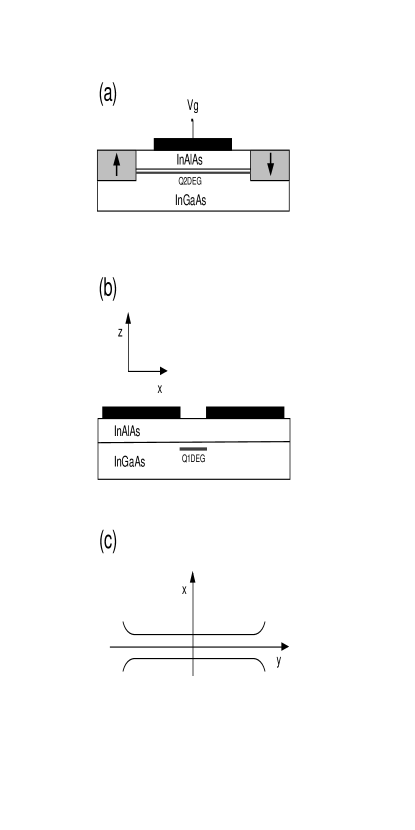
FIG. 1.: (a) Cross sectional schematic of Datta-Das spin modulator device, (b) cross sectional schematic of a split gate device used to create a Q1DEG, (c) diagram of the quasi-one dimensional quantum channel.

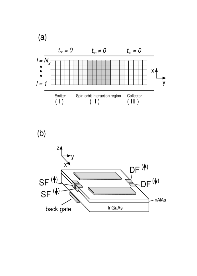
FIG. 2.: (a) Schematic of the tight-binding model for the system. In the shaded areas the spin-orbit interaction is finite, $t_{so}\neq 0$. (b) Schematic of a quasi-one dimensional spin modulator device.

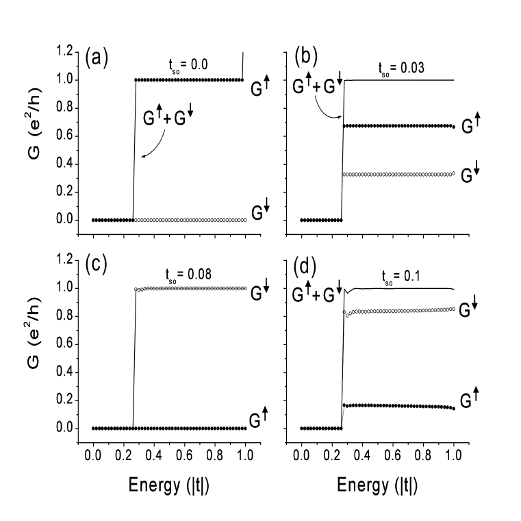
FIG. 3.: Ballistic spin-conductance in units of $e^{2}/h$ against the Fermi energy for a narrow quantum wire of width $W=6a$, showing the spin-modulation for different values of the strength for the spin-orbit hopping parameter. Filled circles $G^{\uparrow}$, empty circles $G^{\downarrow}$, and solid line $G^{\uparrow}+G^{\downarrow}$. In all cases (as in the rest of the calculations), exclusively spin-up polarized electrons are injected to the wire. Note that the spin-conductance modulation is almost independent of the incident Fermi energy as in the model of Datta and Das (Ref. [1]).

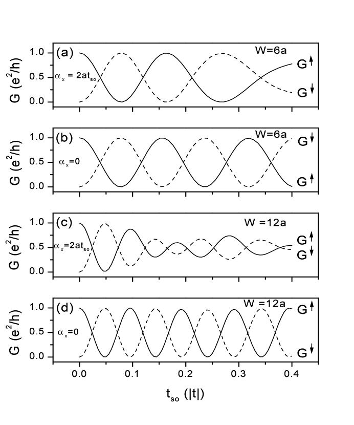
FIG. 4.: Spin-orbit coupling strength dependence of the ballistic spin-conductance, solid line $G^{\uparrow}$, dashed line $G^{\downarrow}$: (a) Narrow wire of $W=6a$, and uniform spin-orbit coupling ($\alpha_{x}=\alpha_{y}=2at_{so}$). (b) Same as in (a) but with $\alpha_{x}=0$ and $\alpha_{y}=2at_{so}$, perfect oscillations are seen for all $t_{so}$. (c) Same as in (a) with $W=12a$. (d) Modulation for $W=12a$, with $\alpha_{x}=0$ and $\alpha_{y}=2at_{so}$. The intersubband mixing clearly changes the otherwise perfectly sinusoidal spin-conductance modulation.

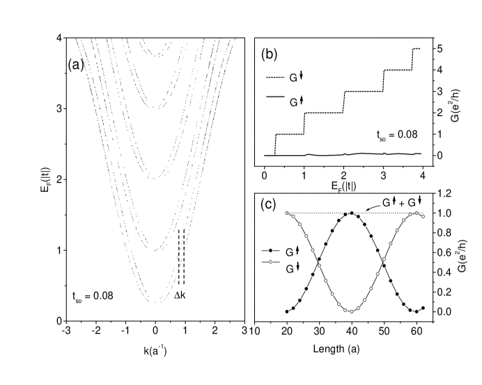
FIG. 5.: (a) Energy subband dispersion for a narrow wire of $W=6a$ and $t_{so}=0.08$ (weak spin-orbit coupling regime). (b) Ballistic spin-conductance for the wire in (a), note that for this value of $t_{so}$, practically all the conductance is due to the precessed spin-down electrons (dashed line), while that for the spin-up is almost zero for all energies (solid line). (c) Oscillating behavior of the spin-conductance versus the effective length of the spin-orbit interaction region, here $t_{so}=0.08$ as well. A wave length of $\lambda=20a$ is extracted from the data.

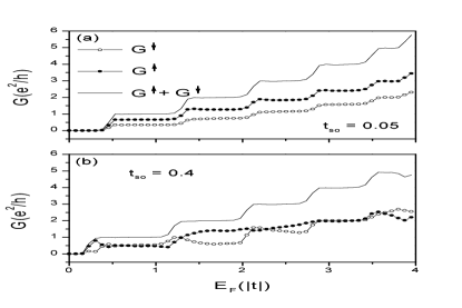
FIG. 6.: Fermi energy dependence of the ballistic spin-conductance (in units of $e^{2}/h$) for a wire of width $W=12a$ and confinement strength (curvature) of the parabolic potential $w_{x}=0.2$. (a) Weak spin-orbit coupling case, $t_{so}=0.05$. (b) Strong spin-orbit coupling case, $t_{so}=0.4$. Filled circles $G^{\uparrow}$, empty circles $G^{\downarrow}$, and solid line $G^{\uparrow}+G^{\downarrow}$.

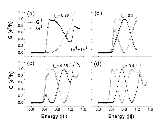
FIG. 7.: Ballistic spin-conductance for the strong spin-orbit coupling regime, ($t_{so}>0.22$) for the wire of Fig. 3. Only the first propagating mode for each spin is shown. In this regime, both $G^{\uparrow}$ and $G^{\downarrow}$ are strongly dependent on the incident Fermi energy, with an oscillating behavior as $t_{so}$ is enhanced, which exhibits the energy dependence of the spin-precession. Cases (c) and (d) are particularly interesting. For $E_{F}\approx 1.0$ in (d) the polarity of the transmitted electrons is reversed (with respect to the injected spin-up polarized electrons) Perfectly polarized spin up or spin down electrons can be emitted from the wire depending on the Fermi energy.

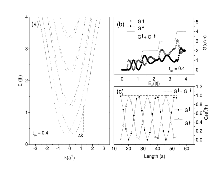
FIG. 8.: (a) Energy subband dispersion for a narrow wire of $W=6a$ and $t_{so}=0.4$ (strong spin-orbit coupling regime). Note that the subbands are no longer parabolic as in weak $t_{so}$ regime, resulting in a $\Delta k\rightarrow\Delta k(E)$. (b) Ballistic spin-conductance for the wire in (a); filled circles $G^{\uparrow}$, empty circles $G^{\downarrow}$, and solid line $G^{\uparrow}+G^{\downarrow}$. The energy dependence is clearly evident here. (c) Oscillating behavior of the spin-conductance versus the effective length of the spin-orbit interaction region ($t_{so}=0.4$) . The wave length of the oscillations is $\lambda\approx 13.8a$.

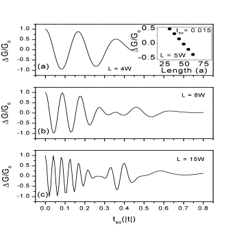
FIG. 9.: Plots of the relative conductance change [$\Delta G/G_{o}=(G^{\uparrow}-G^{\downarrow})/(G^{\uparrow}+G^{\downarrow})$] against the strength of spin-orbit parameter for three different effective lengths of the spin-orbit (Rashba) interaction, $L=4W$, $L=8W$, and $L=15W$, with $W=6a$. Clearly the beat-like behavior is enhanced with $L$, showing the nature of the electron spin-precession induced by the Rashba effect. In the inset of (a) the relative conductance change is plotted as a function of the effective length for a weak spin-orbit hopping parameter, $t_{so}=0.015$. A change in sign for $\Delta G/G_{o}$ as the length is increased is evident showing that the effect of the spin-precession still important for such regime.

REFERENCES

- [1] S. Datta and B. Das, Appl. Phys. Lett. 56, 665, (1990).
- [2] E. I. Rashba, Fiz. Tverd. Tela (Leningrad) 2, 1224 (1960) [Sov. pHys. Solid State 2, 1109 (1960)].
- [3] Y. A. Bychkov and E. I. Rashba, J. Phys, C 17, 6039 (1984).
- [4] J. Nitta, T. Akasaki, H. Takayanagi, and T. Enoki, Phys. Rev. Lett. 78, 1335 (1997).
- [5] J. P. Heida, B. J. van Wees, J. J. Kuipers, T. M. Klapwijk, and G. Borghs, Phys. Rev. B, 57, 11 911 (1998).
- [6] G. Engels, J. Lange, Th. Schäpers, and H. Lüth, Phys. Rev. B 55, 1958 (1997). Th. Schäpers, G. Engels, J. Lange, Th. Klocke, M. Hollfelder, and H. Lüth, J. Appl. Phys. 83, 4324 (1998).
- [7] C.-M. Hu, J. Nitta, T. Akazaki, H. takayanagi, J. Osaka, P. Pfeffer, and W. Zawadski, Phys. Rev. B 60, 7736 (1999).
- [8] D. Grundler, Phys. Rev. Lett. 84, 6074 (2000).
- [9] T. Matsuyama, R. Kürsten, C. Messner, and U. Merkt, Phys. Rev. B 61, 15 588 (2000).
- [10] P. R. Hammar, B. R. Bennet, M. J. Yang, and M. Johnson, Phys. Rev. Lett. 83, 203 (1999). Ibid. J. Appl. Phys. 87, 4665 (2000).
- [11] S. Gardelis, C. G. Smith,C. H. W. Barnes, E. H. Linfield, and D. A. Ritchie, Phys. Rev. B 60, 7764 (1999).
- [12] A. T. Filip, B. H. Hoving, F. J. Jedema, B. J. van Wees, B. Dutta, and S. Borghs, Phys. Rev. B 62, 9996 (2000).
- [13] H. X. Tang, F. G. Monzon, R. Lifshitz, M. C. Cross, and M. L. Roukes, Phys. Rev. B 61, 4437 (2000).
- [14] G. Schmidt, L. W. Molenkamp, A. T. Filip, and B. J. van Wees, Phys. Rev. B 62, R4790 (2000).
- [15] G. Kirczenow, Phys. Rev. B 63 54422 (2001).
- [16] A. V. Moroz and C. H. W. Barnes, Phys. Rev B 60, 14272 (1999).
- [17] R. Winkler, Phys. Rev. B 62, 4245 (2000).
- [18] For the currently typical experimental values of the spin-orbit Rashba parameter, the spin-orbit hopping parameter is estimated to be in the range between to , approximately.
- [19] T. Ando and H. Tamura, Phys. Rev. B, 46, 2332, (1992).
- [20] T. Ando, Phys. Rev. B 44, 8017 (1991).
- [21] S. Nonoyama, A. Nakamura, Y. Aoyagi, T. Sugano, and A. Okiji, Phys. Rev. B, 47 2423 (1993).
- [22] R. Landauer, IBM J. Res. Dev. 1, 223 (1957), R. Landauer, Phys. Lett. 85 A, 91 (1981).
- [23] The Coulomb interactions in a strictly one-dimensional channel with the Rashba interaction have been recently studied within the Tomonaga-Luttinger model by A. V. Moroz, K. V. Samokhin and C. H. W. Barnes, Phys. Rev. B 62, 16900 (2000), and it has been argued by W. Häusler, cond-mat/0101375 that the interactions would enhance the spin-precession at low densities in such models.
- [24] The differential phase shift Eq. (2), is rewritten in terms of the strength of the spin orbit coupling by where is the strength of spin-orbit hopping parameter in units of .
- [25] In contrast to Shubnikov-de Haas (SdH) oscillations the beating in Fig. 9 is a quantum interference effect. If a large number of channels is present more complicated patterns emerge.
- [26] C. M. Hu, J. Nitta, A. Jensen, J. B. Hansen, and H. Takayanagi, (preprint).