[

Internal Fluctuations Effects on Fisher Waves

Abstract

We study the diffusion-limited reaction $A+A\leftrightarrow A$ in various spatial dimensions to observe the effect of internal fluctuations on the interface between stable and unstable phases. We find that, similar to what has been observed in $d=1$ dimensions, internal fluctuations modify the mean-field behavior predictions for this process, which is given by Fisher’s reaction-diffusion equation. In $d>1$ the front displays local fluctuations perpendicular to the direction of motion which, with a proper definition of the interface, can be fully described within the Kardar-Parisi-Zhang (KPZ) universality class. This clarifies the apparent discrepancies with KPZ predictions reported recently.

]

Fluctuations in the macroscopic behavior of reaction-diffusion (RD) systems could play an important role whether these fluctuations are produced by the discrete nature of the elementary constituents (internal) or by environmental random variations (external). Often both type of fluctuations are neglected in the theoretical treatment, thus describing the system by an action-mass type equation (mean-field approximation). Fluctuations in RD systems can, for instance, give rise to instabilities [3], modify the reaction front velocity [4, 5], allow the system to reach new states absent in the mean-field description [6], or produce spatial correlations in the system which in turn can dominate the macroscopic system behavior [7]. While these effects appear in different situations, there is a theoretical and experimental interest in the problem of front propagation in RD systems. The simplest example is that of invasion of an unstable phase by a stable one, which at the mean-field approximation level is described by Fisher’s equation [8]

$$\frac{\partial\rho}{\partial t}=D\nabla^{2}\rho+k_{1}\rho-k_{2}\rho^{2}$$ (1)

where $\rho({\mabold{x}},t)$ is the local concentration (${\mabold{x}}\in{\mathbb{R}}^{d}$) characterizing the system. Equation (1) arises in the macroscopic description of many processes in physics, chemistry and biology and is a generic model for reaction front propagation in systems undergoing a transition from a marginally unstable ($\rho=0$) to a stable ($\rho_{\mathrm{eq}}=k_{1}/k_{2}$) state. Thus, for initially segregated conditions, i.e. $\rho({\mabold{x}})=\rho_{\mathrm{eq}}$ for $x_{\|}\leq 0$ and $\rho({\mabold{x}})=0$ for $x_{\|}>0$ (with ${\mabold{x}}=({\mabold{x}}_{\bot},x_{\|})$, ${\mabold{x}}_{\bot}\in{\mathbb{R}}^{d_{\bot}}$, $x_{\|}\in{\mathbb{R}}$ and $d=d_{\bot}+1$), the solution of (1) is a front invading the unstable phase and propagating along $x_{\|}$ with a constant velocity $v\geq v_{min}=2(k_{1}D)^{1/2}$ which is selected depending on the initial condition according to the “marginal stability criterion” [9]. At the same time, the front broadens until it reaches a finite width $\xi\simeq 8(D/k_{1})^{1/2}$.

The question of how faithfully continuum equation (1) resembles the macroscopic front dynamics of microscopic RD discrete systems has drawn a lot of attention recently. In particular, much attention has been devoted to microscopic stochastic models like $A+A\leftrightarrow A$ or $A+B\to 2A$, where $A$ and $B$ are active species. Discreteness of those systems is responsible for fluctuations in $\rho({\mabold{x}},t)$ and introduces an effective cutoff in the reaction-rates which modifies the properties of the front. Most of the studies have concentrated on observing how the microscopic system approaches the macroscopic behavior described by Eq. (1) in $d=1$ when $N\to\infty$, where $N$ is the number of particles per site [4]. Using van Kampen’s system size expansion [10] or field-theory techniques [11], the mesoscopic dynamics of the microscopic Master equation can be expressed in terms of a Langevin equation which, in the case of the $A+A\leftrightarrow A$ scheme, reads [12]

$$\frac{\partial\rho}{\partial t}=D\nabla^{2}\rho+k_{1}\rho-k_{2}\rho^{2}+\sqrt{(k_{1}\rho-k_{2}\rho^{2})}\ \eta({\mabold{x}},t)$$ (2)

where $\eta({\mabold{x}},t)$ is a uncorrelated white noise, $\left\langle\eta({\mabold{x}},t)\right\rangle=0$, $\left\langle\eta({\mabold{x}},t)\eta({\mabold{x}}^{\prime},t^{\prime})\right\rangle=2\hat{N}^{-1/2}\delta({\mabold{x}}-{\mabold{x}}^{\prime})\delta(t-t^{\prime})$, and $\hat{N}$ is a reference level of number of particles, which is proportional to $N$. In the limit $N\to\infty$, the noise term in (2) (which reflects the fluctuations in the number of particles) vanishes and we recover (1). In this limit, the effective cutoff in the reaction term imposed by the discreteness seems to be the leading contribution, and it is possible to derive corrections to the velocity which yield the well known result $v-v_{\mathrm{min}}\sim 1/\log^{2}N$ [4, 12].

The purpose of this paper is to extend this analysis of discrete microscopic models to higher dimensions. In $d\geq 2$ the front position is given by an interface at $x_{\|}=h({\mabold{x}}_{\bot},t)$ which separates the stable from the unstable domain. Due to the microscopic fluctuations one expects the interface to roughen and its fluctuations to be described asymptotically by the Kardar-Parisi-Zhang (KPZ) [13] equation, which features the simplest and most relevant non-linearity (in the renormalization group sense) that considers local and lateral growth:

$$\frac{\partial h}{\partial t}=\tilde{v}+\tilde{D}\nabla_{\bot}^{2}h+\frac{\lambda}{2}(\nabla_{\bot}h)^{2}+\sqrt{2\sigma}\ \eta_{\bot}({\mabold{x}}_{\bot},t),$$ (3)

where $\eta_{\bot}({\mabold{x}}_{\bot},t)$ is an uncorrelated white noise, and $\nabla_{\bot}$ is the divergence operator defined over the substrate ${\mabold{x}}_{\bot}$. The interface is described by its mean position $\bar{h}(t)$ and its roughness,

$$w^{2}(L_{\bot},t)=\overline{\left\langle[h({\mabold{x}}_{\bot},t)-\bar{h}(t)]^{2}\right\rangle},$$ (4)

where $\left\langle\cdots\right\rangle$ means average over different realizations and the bar denotes average over the substrate ${\mabold{x}}_{\bot}\in L_{\bot}^{d_{\bot}}$ ($L_{\bot}$ is substrate lateral length). As it is well known, in the KPZ equation $w$ obeys a scaling form $w(L_{\bot},t)=t^{\beta}f(t/L_{\bot}^{z})$, where $w\sim t^{\beta}$ if $t\ll L^{z}$ and $w=w_{\mathrm{sat}}\sim L^{\alpha}$ if $t\gg L^{z}$, where $\alpha=\beta z$ is the roughness exponent [14].

However, studies of microscopic realizations of Eq. (1) have questioned the applicability of (3) to describe the interface fluctuations in front dynamics. Riordan et al. [15] studied the $A+A\leftrightarrow A$ scheme in various dimensions concluding that the interface roughens in time for $d_{\bot}\leq d_{\bot,c}=2$ with $\beta_{d_{\bot}=1}=0.27\pm 0.01$ and $\beta_{d_{\bot}=2}\simeq 0$. These values strongly differ from those of KPZ, which are $\beta_{d_{\bot}=1}=1/3$ and $\beta_{d_{\bot}=2}=0.245$[16]. For $d_{\bot}>d_{\bot,c}$, they observed that the interface is flat and described by Eq. (1). However, the determination of these values is hampered by the method used to obtain them, namely, using the front width of the projected density $\rho(x_{\|},t)$ obtained by integrating out all perpendicular dimensions ${\mabold{x}}_{\bot}$. To overcome this problem, Tripathy and van Saarloos [17] studied the interface dynamics in $d_{\bot}=1$ in terms of the coarse-grained density of particles (see below) and obtained $\beta_{d_{\bot}=1}=0.29\pm 0.01$, $\alpha_{d_{\bot}=1}=0.4\pm 0.02$. The authors interpreted this deviation from the KPZ exponents ($\alpha_{d_{\bot}=1}=0.5$) as an effect of the parallel dimension, which cannot be integrated out to obtain an effective interface description in $d_{\bot}$ dimensions and thus, the exponents correspond to those of the KPZ equation in $d_{\bot}+1$ dimensions ($\alpha_{d_{\bot}=2}=0.393$) [16], although the interface is a surface defined in a $d_{\bot}$-dimensional substrate. More recently[18], it has been conjectured that this situation is more general and occurs in the dynamics of the so called “pulled fronts” in which the region ahead of the front is important to determine not only its deterministic properties (like the velocity) but also the fluctuations of the effective interface dynamics [18]. Thus, it is important to check the validity of this conjecture for $d_{\bot}>1$. Although our results are consistent with those in [17], a closer analysis indicates that there is a crossover to the asymptotic behavior of KPZ equation in $d_{\bot}$ dimensions.

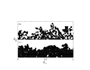
FIG. 1.: (a) Microscopic rules for our model: diffusion (left) and reaction (right). The model is isotropic, i.e., all movements are equally probable in any spatial direction. (b) and (c) Snapshots of the stable domain for $\mu=0.1$ (b), $\mu=0.5$ (c) and $l=5$.

Our simulations are done on a $L_{\bot}^{d_{\bot}}\times L_{\|}$ lattice with $L_{\|}\gg L_{\bot}$. At each point of the lattice we define the occupancy number $n({\mabold{x}},t)$ to be $0,1$ depending whether the site is occupied by a particle or not. At each time step a particle is chosen and can perform any of the processes in Fig. 1a which, in the mean-field approximation, yield $k_{1}=\mu$ and $k_{2}=1+\mu$, i.e. $\rho_{\mathrm{eq}}=\mu/(1+\mu)$ [15]. Diffusion rate is chosen to be $D=1/(2d)$. Initial conditions are set up by distributing particles uniformly over a domain $L_{\bot}^{d_{\bot}}\times L_{\|}^{(i)}$ with density $\rho_{\mathrm{eq}}$ and $L_{\|}^{(i)}$ of the order of hundreds of lattice spacings. The interface is determined using a local coarse-grained density $\rho_{l}({\mabold{x}},t)=l^{-d}\sum_{{\mabold{s}}\in D_{l}}n({\mabold{s}},t)$ where $D_{l}$ is a squared domain of lateral size $l$ around the ${\mabold{x}}$ site. The stable domain of the front is defined by those sites for which $\rho_{l}({\mabold{x}},t)>\frac{1}{2}\rho_{\mathrm{eq}}$ and the position of the interface $h({\mabold{x}}_{\bot},t)$ is the largest value of $x_{\|}$ inside the stable domain for fixed ${\mabold{x}}_{\bot}$ [17].

Simulations show that the interface advances linearly in time, $\bar{h}=vt$, where from we can extract the velocity of the front in any dimension. Values obtained are reported in Fig. 2 and compared with the deterministic prediction $v=v_{\mathrm{min}}=2\sqrt{D\mu}$ of Eq. (1). We recall that in $d=1$ the stochastic model admits an exact solution [19], and the front advances with velocity $v=D\mu$. The difference between both expressions reflects the importance of fluctuations when $N=1$ and $d=1$, and agrees with the breakdown of the approximation $v-v_{\mathrm{min}}\sim\log^{-2}N$ when $N=1$. Interestingly, for $d>1$ we recover the law $v\sim\mu^{1/2}$, although the value is still corrected due to the fluctuations in the number of particles. Nevertheless, the velocity change is smaller when the dimension is increased, as fluctuations get averaged over the transverse dimensions. Moreover, assuming that Eq. (3) holds, we can obtain the value of $\lambda$ by tilting the substrate with an overall slope $m$ and measuring the velocity. As expected we obtain $v(m)=v(0)+\frac{1}{2}v(0)m^{2}$, i.e. $\lambda=v(0)$ [14].

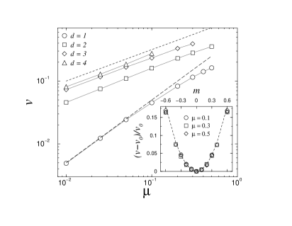
FIG. 2.: Front velocity for different dimensions. Dashed lines are mean-field prediction $v=2(D\mu)^{1/2}$ and $d=1$ exact solution $v=D\mu$. Values for $d\geq 2$ are divided by $2D^{1/2}$. Error bars are smaller than the symbol size. Inset: renormalized velocity as a function of the tilt $m$ for $d_{\bot}=1$. Dashed line is the parabola $m^{2}/2$ and $v_{0}=v(m=0)$.

For $d=2$ the interface roughens subject to internal fluctuations, and the roughness grows like $w(t)\sim t^{\beta}$ until it saturates to a constant value $w_{\mathrm{sat}}\sim L_{\bot}^{\alpha}$ (see Fig. 3). When $\mu=0.1$ we obtain $\beta_{d_{\bot}=1}=0.27\pm 0.01$ and $\alpha=0.40\pm 0.01$, consistent with [17]. Nevertheless, a closer inspection of the data suggests that there is a crossover from non-Gaussian fluctuations at small scales to Gaussian ones at large scales. Although this crossover could be guessed, for instance, from the value of $w_{sat}(L_{\bot})$ for $\mu=0.1$ (which is seen to change its slope in a log-log plot), it becomes clearer if we look at higher moments of the $h({\mabold{x}}_{\bot},t)$ distribution, e.g. the skewness, ${\cal S}=\overline{\left\langle(h({\mabold{x}}_{\bot},t)-\bar{h})^{3}\right\rangle}/w^{3/2}(t)$ and the kurtosis, ${\cal K}=\overline{\left\langle(h({\mabold{x}}_{\bot},t)-\bar{h})^{4}\right\rangle}/w^{2}(t)-3$ when $t\to\infty$ as seen in Fig. 3. Both approach the Gaussian asymptotic regime given by Eq. (3) (i.e. ${\cal S}={\cal K}=0$) when $L_{\bot}\to\infty$. Non-Gaussian fluctuations in the system are due to the vague definition of the interface for small values of $\mu$ and $l$. In Fig. 1b,c we show different snapshots of the stable domain calculated through the coarse-grained density, $\rho_{l}({\mabold{x}})$. It is apparent that when the number of particles inside the domain $D_{l}$ is small, the definition of the interface is vague and implies large steps (or large slopes) which give non-Gaussian fluctuations in $h({\mabold{x}},t)$ at small length scales. Nevertheless these intrinsic fluctuations of the interface are bounded and restricted to small length scales. The measured roughness is naturally decomposed into contributions due to intrinsic fluctuations, $w_{i}$, and long-wavelength fluctuations $w_{0}$ [20, 21]

$$w^{2}(L,t)=w_{i}^{2}+w^{2}_{0}(L,t),$$ (5)

where $w_{i}$ is a non-universal constant that depends on the number of particles, $n_{l}$, inside the domain $D_{l}$ used to determine the interface. Direct fit of expression (5) to a power law when $t\to\infty$ gives lower values of the exponent $\alpha$, while we recover $\alpha=1/2$ when fitting the data in Fig. 3 using expression (5) and assuming that $w_{0}\sim L^{\alpha}$, showing that long-wavelength fluctuations are indeed described by the KPZ equation in $d_{\bot}$ dimensions. In order to reduce the effect of the intrinsic width, we can enlarge the size of the domain and/or the value of $\mu$, as we can see in Fig. 3, where a direct fit to a power law of the data for $\mu=0.1$ and $l=9$ gives $\alpha=0.47\pm 0.01$. In this sense, $n_{l}$ plays the role of a noise-reduction parameter. The situation then is completely reminiscent of what happens in the Eden model [20] and has been also observed in many other RD systems [21].

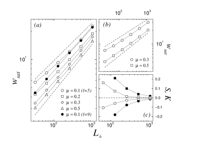
FIG. 3.: (a) Roughness as a function of $L_{\bot}$ for $d=2$. Dashed lines correspond to power laws $L_{\bot}^{\alpha}$ with $\alpha=0.4$ and $\alpha=1/2$. (b) Same as in (a) but for the directed percolation model with $c=0.1$. (c) Skewness (circles) and kurtosis (squares) as a function of $L_{\bot}$ for $\mu=0.1$ (full symbols) and $\mu=0.5$ (open symbols). Error bars are about 0.05 but have been omitted for clarity reasons.

In higher dimensions results are analogous. In $d=3$ we do observe a significant increase in the roughness with $L_{\bot}$, contrary to what was observed in [15]. The reason for this discrepancy is that the roughness measured in [15] is also a linear combination of the long-wavelength roughness $w_{0}(L_{\bot},t)$ and the front width, $\xi$. In $d=2$ we have $w_{0}(L_{\bot},t)>\xi$, while in $d=3$, $w_{0}(L_{\bot},t)\simeq\xi$ (for the simulated values of $L_{\bot}$), and this is responsible for an apparent value of $\alpha_{d_{\bot}=2}\simeq 0$. Actually, using the structure factor $S({\mabold{q}_{\bot}},t)=\langle\hat{h}({\mabold{q}_{\bot}},t)\hat{h}(-{\mabold{q}_{\bot}},t)\rangle$ where $\hat{h}({\mabold{q}_{\bot}},t)$ is the Fourier transform of $h({\mabold{x}}_{\bot},t)$, we observe in Fig. 4 a crossover to the asymptotic scaling $S({\mabold{q}_{\bot}}\ll 1,t\to\infty)\sim q^{-d-2\alpha}$ with $\alpha_{d_{\bot}=2}=0.393$ of KPZ equation [oscillations for $q>1$ are due to artificial correlations in $h({\mabold{x}},t)$ introduced by the coarse-grained density]. Finally, in $d=4$ we observe two different behaviors: for small values of $\mu$ the roughness seems to saturate to a value independent of $L_{\bot}$ while for $\mu=0.5$ we recover the asymptotic prediction of Eq. (3), $\alpha_{d_{\bot}=3}=0.313$ [16]. This difference may be due to the existence of a phase transition for the KPZ equation in $d_{\bot}>2$, in which, depending on the control parameter $g^{2}=\lambda^{2}\sigma D^{-3}$, the interface is flat (for $g<g_{c}\simeq 6.28$) or rough (for $g>g_{c}$). Our results suggest that the interface is flat for $\mu=0.1$ (i.e. $w^{2}$ does not scale with $L_{\bot}$) while it is rough for $\mu=0.5$, although more simulations are needed.

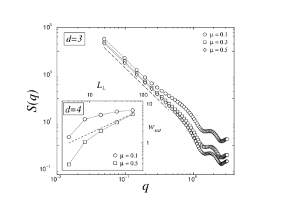
FIG. 4.: Structure factor as a function of the wave number $q$ for $d=3$ and $L_{\bot}=128$. Dashed line correspond to the KPZ prediction in $d_{\bot}=2$, $S(q)\sim q^{-2+2\alpha}$ with $\alpha=0.393$. Inset: Saturation roughness as a function of $L_{\bot}$ in $d=4$. Dashed line corresponds to the power law $L_{\bot}^{\alpha}$ with $\alpha=0.313$.

We have also performed simulations for the $N=1$ directed percolation model in which the decay $A\to\emptyset$ is allowed with rate $c$. The model presents a non-trivial phase transition for finite values of $\mu$ and $c$ in which the stable state changes from an active ($\rho_{\mathrm{eq}}\neq 0$) to an absorbing state ($\rho_{\mathrm{eq}}=0$) for $d\leq 4$ [22]. In this case, the mesoscopic dynamics of the system are given by [7, 11]

$$\frac{\partial\rho}{\partial t}=D\nabla^{2}\rho+k_{1}\rho-k_{2}\rho^{2}+\sqrt{k_{3}\rho}\ \eta({\mabold{x}},t),$$ (6)

the only difference with (2) being the form of the noise term. Away from the transition point (which occurs when $\mu=0.22\pm 0.01$ for fixed value of $c=0.1$), interface fluctuations behave similarly to the previous model (see Fig. 3b), confirming that our results do not depend on the specific choice of the microscopic rules, as long as the mean-field limit of them coincides with (1).

In summary we have studied two microscopic stochastic realizations of Fisher’s equation with $N=1$. It has been shown that with a proper definition of the interface, long-wavelength fluctuations are fully described within the KPZ scaling in $d_{\bot}$ substrate dimensions. Thus, for $d\leq 4$ there is not an upper critical dimension above which (1) is valid. Only for $d=4$ does the interface seem to undergo a phase transition between a flat interface [which can now be explained by (1)] and a rough phase, depending on the microscopic parameters.

Finally, we comment on the possibility to observe the conjecture in [18] using microscopic RD systems. It is possible to argue that the results in this paper deviate from those of the conjecture because the limit $N\to\infty$ in which Eq. (1) is valid has not been reached. Thus for large values of $N<\infty$ [23] we should be able to observe a crossover to the universality class proposed in [18]. However, the conjecture requires that the noise term scales as $\rho\eta({\mabold{x}},t)$ when $\rho\to 0$, which we call multiplicative noise. This type of noise can be obtained, for instance, assuming that the reaction rates fluctuate in time due to environmental variations (external noise). As argued in [24], it is impossible to find such an internal noise in a microscopic RD model. For example, in the models analyzed here, the noise term scales as $\rho^{1/2}\eta({\mabold{x}},t)$ for $\rho\to 0$ [see Eqs. (2) and (6)]. Thus, even if the parallel dimension is relevant to determine the interface properties of the front for large values of $N$, we expect internal fluctuations to give a different universality class from the one proposed in [18].

We thank J. L. Cardy for illuminating discussions and D. B. Abraham, A. Buhot, R. Cuerno, J. P. Garrahan, W. van Saarloos and G. Tripathy for useful comments. This work has been supported by EPSRC Grant No. GR/M04426 and EU Grant No. HPMF-CT-2000-00487.

Note added: After completion of this paper we became aware of a recent preprint, R. A. Blythe and M. R. Evans, cond-mat/0104393, in which a similar crossover is found for a model in the directed percolation universality class of (6) in $d_{\bot}=1$.

REFERENCES

- [1]
- [2] E-mail address: e.moro1@physics.ox.ac.uk
- [3] D. A. Kessler and H. Levine, Nature 394, 556 (1998).
- [4] E. Brunet and B. Derrida, Phys. Rev. E 56, 2597 (1997).
- [5] J. Armero, J. Casademunt, L. Ramírez-Piscina and J. M. Sancho, Phys. Rev. E 58, 5494 (1998).
- [6] J. García-Ojalvo and J. Sancho, Noise in spatially Extended Systems (Springer-Verlag, New York, 1999).
- [7] J. L. Cardy and U. C. Täuber, J. Stat. Phys. 90, 1 (1998), and references therein.
- [8] R. A. Fisher, Ann. Eugenics VII, 355 (1936); J. D. Murray, Mathematical Biology, (Springer, Berlin, 1989).
- [9] E. Ben-Jacob et al. Physica D 14, 348 (1985). W. van Saarloos, Phys. Rev. A 39, 6367 (1989); G. C. Paquette et al. Phys. Rev. Lett. 72, 76 (1994).
- [10] C. W. Gardiner, Handbook of Stochastic Methods, (Springer, Berlin, 1996).
- [11] M. Doi, J. Phys. A 9, 1479 (1976); L. Peliti, J. Phys. (Paris) 46, 1469 (1985); D. C. Mattis and M. L. Glasser, Rev. Mod. Phys. 70, 979 (1998).
- [12] L. Pechenik and H. Levine, Phys. Rev. E 59, 3893 (1999).
- [13] M. Kardar, G. Parisi, and Y.C. Zhang, Phys. Rev. Lett. 56, 889 (1986).
- [14] A.-L. Barabási and H. E. Stanley, Fractal concepts in surface growth (Cambridge Univ. Press, Cambridge, 1995); J. Krug, Adv. Phys. 46, 129 (1997).
- [15] J. Riordan, C. R. Doering and D. ben-Avraham, Phys. Rev. Lett. 75, 565 (1995).
- [16] E. Marinari, A. Pagnani, G. Parisi, J. Phys. A: Math. Gen. 33, 8181 (2000).
- [17] G. Tripathy and W. van Saarloos, Phys. Rev. Lett. 85, 3556 (2000).
- [18] G. Tripathy, A. Rocco, J. Casademunt and W. van Saarloos, cond-mat/0102250
- [19] C. R. Doering, M. A. Burschka, and W. Horsthemke, J. Stat. Phys. 65, 953 (1991);
- [20] D. E. Wolf and J. Kertész, J. Phys. A 20, L257 (1987); J. Kertész and D. E. Wolf, ibid. 21, 747 (1988).
- [21] M. Tammaro and J. W. Evans, J. Chem. Phys. 108, 762 (1998); F. Chávez et al., ibid. 110, 8119 (1999).
- [22] See H. Hinrichsen, Adv. Phys. 49, 815 (2000) for a recent review of directed percolation and related work.
- [23] Note that has to be finite, because in the limit , noise terms in (2) and (6) vanish and hence the interface does not fluctuate.
- [24] M. J. Howard and U. C. Täuber, J. Phys. A: Math. Gen. 30 7721 (1997); M. A. Muñoz, Phys. Rev. E 57, 1377 (1998).