Freezing in Ising Ferromagnets

Abstract

We investigate the final state of zero-temperature Ising ferromagnets which are endowed with single-spin flip Glauber dynamics. Surprisingly, the ground state is generally not reached for zero initial magnetization. In two dimensions, the system either reaches a frozen stripe state with probability $\approx 1/3$ or the ground state with probability $\approx 2/3$. In greater than two dimensions, the probability to reach the ground state or a frozen state rapidly vanishes as the system size increases and the system wanders forever in an iso-energy set of metastable states. An external magnetic field changes the situation drastically – in two dimensions the favorable ground state is always reached, while in three dimensions the field must exceed a threshold value to reach the ground state. For small but non-zero temperature, relaxation to the final state first proceeds by the formation of very long-lived metastable states, similar to the zero-temperature case, before equilibrium is reached.

PACS Numbers: 64.60.My, 05.40.-a, 05.50.+q, 75.40.Gb

I Introduction

A Background

Despite extensive study[1, 2], several fundamental questions about the kinetic Ising model with Glauber dynamics still remain unanswered [3]. In this paper, we investigate the following basic issue: What is the final state of a finite Ising-Glauber spin system when it is suddenly quenched from infinite temperature to zero temperature[4]? An infinite system undergoes coarsening, that is, the spins organize into a coarsening domain mosaic of up and down spins, with the characteristic domain length scale growing as $t^{1/2}$. For a finite system, this coarsening is interrupted when the typical domain size reaches the system size $L$. Rather unexpectedly, this interruption can cause the system to get stuck in an infinitely long-lived metastable state. In two dimensions, it appears that, as $L\to\infty$, this probability of getting stuck is approximately $1/3$, while for $d\geq 3$ the ground state is never reached.

To provide context for the question of the ultimate fate of the Ising-Glauber system, consider the limiting cases of $d=1$ [4, 5] and $d=\infty$. For a linear chain of length $L$ which initially contains $pL$ up spins and $(1-p)L$ down spins, the final state of the system follows from two facts. First, the average magnetization is conserved under Glauber dynamics [1, 5] and second, the only possible final states are all spins up or all spins down; there are no metastable states in one dimension. To achieve a final magnetization which equals the initial magnetization, a fraction $p$ of all realizations must end with all spins up and the complementary fraction must end with all spins down. Thus the probability $P(p)$ to ultimately have all spins up as a function of the initial concentration of up spins $p$ is simply $P(p)=p$. A very different result holds in the mean-field limit. A simple realization of this limit is the complete graph, in which each spin interacts with every other spin in the system. Here, a non-zero magnetization makes it energetically favorable for any minority spin to flip, so that the majority phase quickly fills the system for all $p\neq 1/2$. Therefore on the complete graph, $P(p)$ is simply the step function $P(p)=\theta(p-1/2)$.

We argue that in two and higher dimensions the probability that one phase eventually wins also converges to a step function in $p-1/2$ but with strange anomalies when $p=1/2$. As mentioned above, the system has a non-zero probability of getting stuck in a metastable state which consists of two or more straight stripes in two dimensions. In greater than two dimensions, the probability that the ground state is reached quickly vanishes with system size. Intriguingly, the final state is not static, but rather consists of stochastic “blinkers”. These are localized sets of spins which can flip ad infinitum without any energy cost. Thus the system wanders forever on a connected set of equal-energy states defined by these blinkers. In the categorization proposed by Newman and Stein[3], the Ising system in high spatial dimension is of type ${\cal M}$ (“mixed”) in that a fraction of the spins flip a finite number of times, while the complementary fraction flip infinitely often.

We also study the fate of the Ising system in the presence of an external magnetic field. The imposition of a field leads to bootstrap percolation phenomena[6, 7]. In two dimensions, an infinitesimal field is sufficient to drive the system to the energetically favorable ground state; this is the analog of the percolation threshold being equal to 1 in $n=3$ bootstrap percolation on the square lattice. In three dimensions, the energetically favorable ground state is reached only if the field exceeds a threshold value, while for weaker fields, a transition between phase coexistence and field alignment occurs as a function of the initial concentration of field-aligned spins. This transition again can be described in terms of bootstrap percolation.

Finally, we examine the relaxation at non-zero temperatures. While the system eventually reaches equilibrium, the aforementioned metastable states continue to play a significant role in the relaxation. For example in $d=2$ and temperatures up to approximately $0.2T_{c}$, there is a large time range for which the relaxation is close to that of the zero-temperature system. If a metastable stripe configuration happens to form, a time of the order of $L^{3}\,e^{4J/kT}$, where $J$ is the interaction strength between spins, must elapse before the system can escape this metastable state and reach equilibrium. We expect that analogous metastable states will influence the long-time relaxation even more strongly in higher dimensions.

B The Model

We study the homogeneous ferromagnetic Ising model with Hamiltonian ${\cal H}=-J\sum_{\langle ij\rangle}\sigma_{i}\sigma_{j}$, where $\sigma_{i}=\pm 1$ and the sum is over all nearest-neighbor pairs of sites $\langle ij\rangle$. The spins are initially uncorrelated, corresponding to an initial temperature $T=\infty$. The $T=\infty$ limit implies that the fraction of up and down spins are equal. Because we are interested in subtle effects associated with zero initial magnetization, we prepare our systems with fixed magnetization, rather than fixed probability for the orientation of each spin. Thus every initial configuration has $L^{d}/2$ up spins and $L^{d}/2$ down spins. We also consider the straightforward generalization to non-zero magnetization by having $p\times L^{d}$ up spins and $(1-p)\times L^{d}$ down spins, where $p$ is the initial fraction of up spins.

The spins evolve by zero-temperature Glauber dynamics[1], i. e., we view the system as being suddenly quenched from $T=\infty$ to $T=0$. (In Sect. IV, we will also consider the $T>0$ case.)  For each initial spin configuration, one realization of the dynamics was performed until the final state was reached. We focus on $d$-dimensional hypercubic lattices with linear size $L$ and periodic boundary conditions. We choose these lattices to avoid the pathologies associated with odd-coordinated lattices, where stable convex islands of minority spins readily form and the system always freezes into a disordered state[3, 4]. Most of our results continue to hold for free boundary conditions and on arbitrary even-coordinated lattices.

Glauber dynamics at zero temperature is implemented by picking a spin at random and computing the energy change $\Delta E$ if this spin were to flip. If $\Delta E$ is greater than, equal to, or less than zero, the spin flip is accepted with probability $1$, $1/2$ and $0$, respectively. After each such event, the time is incremented by $1/L^{d}$. At long times this procedure is prohibitively slow because there are relatively few flippable spins – those with $\Delta E\leq 0$. Thus we track and randomly pick only flippable spins, and then update the time by $1/(\hbox{number of flippable spins})$. This implementation guarantees that in one time unit, each spin attempts one flip on average.

The rest of this paper is organized as follows. In Sect. II we describe geometric properties of the final state in various spatial dimensions including the distribution of magnetization and energy in the final state, as well as the influence of an external magnetic field in determining the final state. The number of metastable states as a function of the spatial dimension is estimated in Sect. III. In Sect. IV, we discuss the finite-temperature evolution in two and three dimensions. We conclude in Sect. V with a summary and some open questions.

II Final State Geometry

We first address the following basic question: what is the probability $P(p)$ that the Ising system with $p\times L^{d}$ up spins in the initial state which is then suddenly quenched to $T=0$ will ultimately have all spins up? One could imagine three possible outcomes:

• $P(p)$ is a monotonically increasing function of $p$.

• $P(p)=0$ for sufficiently small initial concentration of up spins $0\leq p\leq p_{c}$; $P(p)$ increases monotonically for $p_{c}<p<1-p_{c}$; $P(p)=1$ for $p\geq 1-p_{c}$.

• $P(p)$ is the step function $P(p)=\theta(p-1/2)$.

In one dimension $P(p)=p$, i. e., the first scenario applies. In this section we shall argue that in higher dimensions the third scenario is realized.

If the third scenario applies, then additional considerations are needed to determine $P(1/2)$. The behavior at $p=1/2$ is of paramount interest because in a genuine $T=\infty$ initial state the concentrations of up and down spins are equal (when initial temperature exceeds $T_{c}$, these concentrations are also equal as long as there is no external magnetic field). A general belief is that in the thermodynamic limit the system always reaches one of the ground states. The symmetry between up and down phases then implies $P(1/2)=1/2$. This assertion turns out to be wrong for all $d\geq 2$; the two-dimensional system does not always reach the ground state while in higher dimensions the system never reaches the ground state as $L\to\infty$.

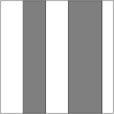
FIG. 1.: Four-stripe metastable state in two dimensions.

The crucial difference between one and higher dimensions is that no metastable states exist in one dimension while there are numerous metastable states in higher dimensions. The existence of such states[8, 9, 10] is easy to visualize in two dimensions, where any stripe of width $\geq 2$ which traverses the entire system is obviously stable at zero temperature (Fig. 1). However, it is not a priori clear what is the basin of attraction of these metastable states and the relative size of this basin compared to the basin of attraction to the ground states. We now turn to numerical results which indicate that metastable states profoundly affect the fate of arbitrarily large higher-dimensional zero-temperature Ising systems.

A Two Dimensions

1 Stripe state in zero magnetic field

Our simulations indicate that the system with zero initial magnetization reaches a stripe state with a non-zero probability as $L\to\infty$ (Fig. 2). Linear extrapolation of the last 4 data points for the probability of reaching the stripe state, $P_{\rm str}(L)$, versus $L$ gives $P_{\rm str}(\infty)\approx 0.315$ and $0.344$ on the square and triangular lattices, respectively.

FIG. 2.: Probability that an $L\times L$ system ($\square$ square lattice, $\Delta$ triangular lattice) eventually reaches a stripe state, $P_{\rm str}(L)$, as a function of $1/\log_{2}L$ for $L$ up to 512. Each data point, with error bars smaller than the size of the symbol, is based on $\geq 10^{5}$ initial spin configurations.

The stripe state can contain an arbitrary even number of stripes. For the square system, we typically obtain two stripes of similar widths. Metastable states with more than two stripes appear very rarely. For example, the probability of reaching the four-stripe state grows very slowly with $L$ and is less than $0.07\%$ for $L=200$. We can gain a qualitative understanding for the dependence of the probability of obtaining $k$ vertical stripes in the final state, $P(k,A)$, by analyzing a general rectangular system of size $AL\times L$ with fixed aspect ratio $A$ (and taking the $L\to\infty$ limit as usual). For example, for $A=9$ and $L=32$ the final probabilities $P(k,A)$ are approximately 0.0028, 0.101, 0.35, 0.36, and 0.15, for $k=0,2,\ldots,8$. There is also a probability approximately 0.034 that a horizontal stripe forms. In general, the probability $P(k,A)$ appears to be peaked around $k_{\rm max}\propto A$. Invoking the natural assumption of analyticity in $A$ then implies that the probabilities $P(k,A)$ of $k$-stripe states are positive for all (even) $k$ and arbitrary aspect ratio $A$.

Our data are insufficient to probe the $k$-dependence of $P(k,A)$ but qualitatively $P(k,A)$ decays faster than exponentially. This behavior seems to be similar to that of the number of spanning clusters on the rectangles of fixed shape at the percolation threshold. In that problem, a wide consensus that only one spanning cluster exists has been recently disproved by numerical[11] and theoretical[12] evidence. We now employ an argument similar to the one of Ref. [12] in the context of spanning clusters to estimate the large-$k$ behavior of $P(k,A)$. Specifically, we consider the probability $P_{h}(k,A)$ to reach a state with $k$ horizontal stripes (all $k$ stripes in the direction of the length $AL$). Imagine now dividing the rectangle into two equal rectangles of size $AL\times L/2$ each. In the large-$k$ limit, the dominant contribution to $P_{h}(k,A)$ comes from situations where approximately $k/2$ stripes traverse each of the rectangles. This implies

$$P_{h}(k,A)\sim[P_{h}(k/2,2A)]^{2},$$ (1)

which may be iterated to give

$$P_{h}(k,A)\sim[P_{h}(2,Ak/2)]^{k/2}.$$ (2)

The quantity on the right-hand side $P(2,Ak/2)$ is the probability to have a stripe which traverses a rectangle of dimension $AL\times 2L/k$ in the long direction. Here we have assumed that the probabilities $P_{h}(k,A)$ depend weakly on the system size $L$ and do not vanish in the thermodynamic limit. If we take $L\sim k$ as the width of the original rectangle, then the rectangle $AL\times 2L/k$ has a small finite width and a length of order $Ak$. This rectangle is so narrow that a stripe can occur only if existed in the initial state. This clearly occurs with probability $2^{-2\times{\rm length}}\sim e^{-Ak}$. By substituting $P(2,Ak/2)\sim e^{-Ak}$ into Eq. (2) we deduce that

$$P_{h}(k,A)\sim e^{-{\rm const.}\times Ak^{2}}.$$ (3)

Thus $P(k,A)$ has a Gaussian tail. This explains why four and higher-stripe states are almost never seen in our simulations for the square system. In the following, we always consider square (or hypercubic) systems.

Consider now an Ising system with a small difference between the number of up and down spins. We study two basic quantities: (i) the probability ${\cal M}(p,L)$ that the minority phase wins, that is, the sign of the magnetization in the final (ground) state is opposite to that in the initial state, and (ii) the probability ${\cal S}(p,L)$ that the system reaches a stripe state. Both these quantities exhibit scaling when $L$ diverges and the the initial magnetization $m_{0}=2p-1$ vanishes such that the combination $z\equiv L|2p-1|^{\nu}$ is kept constant. For ${\cal M}(p,L)$, the best data collapse is achieved with $\nu\approx 1.5$ while for ${\cal S}(p,L)$ the best data collapse is achieved with $\nu\approx 1.35$. Further, ${\cal M}(z)$ appears to be an exponentially decaying function of $z$ while ${\cal S}(z)$ appears to decay even more quickly (Fig. 3). The exponential behavior is not surprising in view of the analogy to the spanning probability in percolation. Indeed, consider the extreme case case of percolation with $p\to 0$. Then a spanning cluster of the minority phase exists with probability $\propto p^{L}$, i. e., it decays exponentially with system size. This argument makes it plausible that ${\cal M}(z)$ and ${\cal S}(z)$ also decay at least as fast as exponentially with $L$ and thence with $z$.

FIG. 3.: Probability that the minority phase wins (lower) or a stripe state is reached (upper) as a function of $L|p-1/2|^{\nu}$, with $\nu=1.5$ and $\nu=1.35$ respectively. Data are based on systems with $L\leq 200$ and $\geq 5\times 10^{4}$ initial configurations.

Overall we conclude that in two dimensions, the initial majority phase always wins in the limit $L\to\infty$. Thus $P(p)=\theta(p-1/2)$ in two dimensions, just as in the mean-field limit. This suggests that $P(p)$ may well be a step function for all spatial dimensions $d\geq 2$ when $L=\infty$.

2 Finite magnetic field

It is also instructive to investigate the effect of a finite external magnetic field $h$ on the fate of the system. In two dimensions there are two distinct field ranges: (i) weak fields $0<h<2J$, and (ii) strong fields $2J<h$. A weak field modifies the dynamics of spins which have two misaligned neighbors. In zero field such spins flip with rate 1/2, while in a weak field they can only flip parallel to the field. This means, for example, that kinks on interfaces move in only one direction rather than diffusing (Fig. 4). For strong fields, down spins which have 3 misaligned neighbors can now flip parallel to the field and the system ends up in the field-aligned ground state.

FIG. 4.: In a weak positive field an interface kink can move only to the right, while in zero field this kink diffuses.

The most interesting case is that of weak field and a small initial concentration of up spins, where the system consists of small clusters of up spins in a background of down spins. Due to the unidirectional kink motion on interfaces, clusters of up spins can grow until each fills out its convex hull (Fig. 5). If the convex hull of one cluster overlaps with either another up cluster (or its convex hull), then the resulting aggregate can expand further to fill out this enlarged convex hull. If there is yet another cluster (or convex hull) within this expansion zone, growth continues.

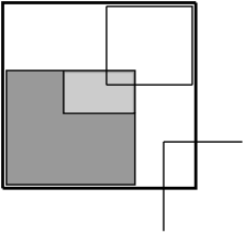
FIG. 5.: Expansion of a cluster of up spins (dark shaded) in a weak magnetic field $h<2J$. The convex hull (union of dark and light shaded regions) overlaps with the cluster on the upper right. The convex hull of this aggregate (outer rectangle) then overlaps with yet another cluster, leading to continued expansion.

This growth process is essentially the same as bootstrap percolation [6], in which a lattice is randomly occupied, say with initial density $\rho_{0}$, and then all sites that do not have at least $n$ occupied neighbors are removed. This deletion step is then repeated until no more sites can be removed. The case $n=3$ is essentially identical to our weak-field system, with spins antiparallel to the field playing the role of occupied sites in bootstrap percolation. In $n=3$ bootstrap percolation, all occupied sites will eventually be removed for $L\to\infty$, even if $\rho_{0}$ is arbitrarily close to 1. Translating this to the Ising system, we conclude that for any non-zero concentration of up spins, the system will evolve to the ground state with $m=1$ in the thermodynamic limit.

B Three Dimensions

1 “Blinkers” in zero magnetic field

On the simple cubic lattice, the probability to reach the ground state, $P_{\rm gs}(L)$, decreases rapidly with the system size (Fig. 6). For example, $P_{\rm gs}(L)\approx 0.001$ for $L=30$. Perhaps even more surprising is that the final state of the system for large $L$ is not geometrically static! Instead, the system contains blinkers – localized sets of spins which can flip indefinitely with no energy cost.

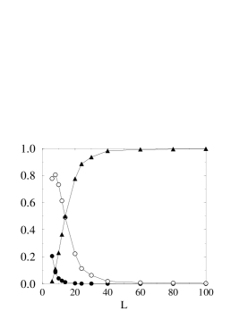
FIG. 6.: Probability that the system reaches the ground state (dots), a frozen metastable state (circles), or a blinker state (triangles) as a function of the linear dimension. The number of realization is $\geq 10^{4}$ for each system size. The lines are a guide for the eye.

To appreciate the nature of blinkers, we first describe the geometry of the frozen metastable states. For initial concentration of up and down spins $p=1/2$ (which is much greater than the percolation threshold $p_{c}\approx 0.3116$ [7]), both the up and down spins percolate in all three coordinate directions in the final state. For example, for cubes with $L=20$, 30 and 40, the probability that both phases percolate in all three directions equals 0.83, 0.92 and 0.97 respectively. Numerically the number of distinct spin clusters almost always equals 2 – there are no small clusters of spins.

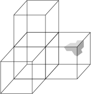
FIG. 7.: A 3-arm star which percolates in all coordinate directions. This cluster contains four cubic blocks of linear dimension $L/2$ in an $L\times L\times L$ system with periodic boundary conditions. The other phase occupies the remaining half of the cube volume. A convex corner (for free boundary conditions) is shown shaded.

To visualize these percolating spin clusters, consider each spin as occupying a unit cube. A cluster must then have no convex corners to be stable (Fig. 7); a spin at such a corner can flip freely and generate additional convex corners. The generic configuration which permits two clusters of oppositely-oriented spins, each devoid of convex corners, to percolate in all three directions has the form of two interpenetrating 3-arm stars (Fig. 7). Each arm is oriented along one coordinate direction and joins onto itself because of the periodic boundary condition, so that there are no convex corners. This is the 3-dimensional analog of stripes on the square lattice.

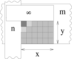
FIG. 8.: Stochastic blinker on the cubic lattice. The shaded region of size $x\times y\times(n-m)$ contains a fluctuating interface which can range between all spins up and all spins down.

From the 3-arm star, a blinker arises when the arms have different cross-sectional areas, as sketched in Fig. 8. Here we view the percolating cluster of up spins as a building with an $m$-storey section (marked $m$), an adjacent $n$-storey section (with $n>m$), and a section (marked $\infty$) which wraps around the torus in the vertical direction and rejoins the building on the ground floor. The wiggly lines indicate wrapping around the torus in the $x$- and $y$-directions. This 3-arm star structure has no convex corners and thus cannot shrink under Glauber kinetics. The shaded portion of Fig. 8 supports a blinker. This blinker starts at the upper left corner of the shaded region of height $m$, where it costs zero energy to flip the heavy shaded spin. Once this spin flips, its three nearest neighbors (two light shaded and one just above the dark-shaded spin in Fig. 8) can also flip with no energy cost. Continuing this process gives rise to a fluctuating interface in the shaded parallelepiped that is bounded by the states of all spins up and all spins down. Thus a blinking state wanders forever by transitions between connected metastable configurations with the same energy.

FIG. 9.: Illustration of blinker topology on a 6-coordinated Cayley tree. The blinker, namely, the bond between the misaligned spins (wiggly line) undergoes a random walk.

Blinkers can be visualized more simply on an even-coordinated Cayley tree (Fig. 9). Consider, for example, a 6-coordinated tree in which each spin in a finite segment (thick lines) feels zero exchange field from the 4 neighboring spins which belong to separate chains. The ends of this segment are terminated by 5 additional chains with at least 4 spins in agreement for these chains. This segment is effectively a finite one-dimensional chain with the endpoints fixed to be in opposite states so that a blinker lives forever.

Amusingly, blinkers are much more prominent in the Potts model with Glauber kinetics, where they arise even in two dimensions. The Hamiltonian of the $Q$-state Potts model is ${\cal H}=-J\sum_{\langle ij\rangle}\delta_{\sigma_{i}\sigma_{j}}$. Here $\sigma_{i}$ denotes the Potts variable at site $i$ which can assume $Q$ distinct values and the sum is over all nearest-neighbor pairs of sites[13]. The zero-temperature Glauber kinetics is analogous to the Ising case, i. e., a spin flips to agree with the majority of its neighbors. In cases of a “tie”, flips occur with equal rates; for example, if half the neighbors of a given spin are in one state and the other half are in a different state then the spin flips to one of these two states with equal probability.

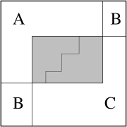
FIG. 10.: Generic stochastic blinker in the kinetic three-state Potts model on the square lattice. The shaded region can flip between all spins in the $A$ and $C$ states, while all the remaining spins are stable since they have at most one misaligned neighbor. A representative position of the $AC$ interface in the shaded region is shown.

To appreciate the existence of blinkers, consider the three-state Potts model in two dimensions and assume that all three phases have the same initial concentration (this again corresponds to a $T=\infty$ initial state). This system can reach a metastable state which contains blinking domains, as illustrated in Fig. 10. Similar to the case of the Ising system on the cubic lattice, the shaded region can blink between having all spins in the $A$ or the $C$ states. While it was previously argued[9, 10] that domains can become pinned for quenches to $T=0$ when $Q\geq 3$, our simulations of the $Q=3$ Potts model indicate that the probabilities to reach the ground state and a frozen state decrease with the system size and apparently approach to zero as $L\to\infty$. In short, the Potts system gets pinned in a blinking state rather than in a frozen state.

2 Finite magnetic field

An external magnetic field again drastically changes the final state of the system. On the cubic lattice there are now two critical fields, $h_{1}=2J$ and $h_{2}=4J$, which demarcate different behaviors. The regime $0<h<2J$ corresponds to $n=4$ bootstrap percolation for the clusters of spins antiparallel to the field. In the language of the Glauber kinetics, this means that spins with initially three misaligned neighbors must align with the field. These spins, when flipped, fill in concavities and eventually complete convex corners, as illustrated in Fig. 11.

For $0<h<2J$, there is a threshold initial concentration of up spins, $p_{h}$, below which finite droplets of up spins, with each spin having at least three aligned neighbors, freeze. For $p>p_{h}$, up spins eventually percolate due to the infilling of concavities, which leads to the merging of clusters of up spins and ultimately the ground state is reached. Our simulations give $p_{h}$ significantly smaller than $p_{c}\approx 0.3116$ for site percolation on the cubic lattice, in qualitative agreement with Ref. [6].

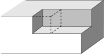
FIG. 11.: Cluster of up spins with a concave trough. This is sequentially filled in, for $0<h<2J$, by flipping spins which each have 3 misaligned neighbors. The dashed cube represent the spin which is about to flip.

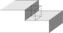
FIG. 12.: Cluster of up spins with a concave interface. The energy cost of flipping the indicated spin is $4J-2h$; thus, this spin will flip when $h>2J$.

The regime $2J<h<4J$ corresponds to $n=5$ bootstrap percolation. It is now possible to flip a spin adjacent to a straight but concave interface (Fig. 12). This filling ultimately allows a cluster of up spins to systematically expand and fill its convex hull. This then leads to a similar picture to $n=3$ bootstrap on the square lattice, in which coalescence of convex hulls of neighboring clusters leads to a final state where all spins are aligned with the field for any initial magnetization. Finally for $h>4J$, even a single up spin nucleates the growth of additional up spins and the system quickly reaches the ground state with all spins pointing up.

C Final Magnetization Distribution

In two dimensions, we have seen that the final state is either the ground state or a stripe state in which there are typically two stripes of approximately the same width. This qualitative observation can be made more precise by studying the magnetization distribution of the final state. Systems which reach the ground state give $m=+1$ or $-1$, while systems which reach the stripe state lead to a continuous component of the final magnetization distribution which is peaked about 0. The width of this peak gradually narrows as the system size increases, but appears to converge to a finite limit as $L\to\infty$.

FIG. 13.: Final magnetization distribution in (a) $d=2$ and (b) $d=3$. The number of configurations is $\geq 10^{5}$ for every system size in $d=2$, and $\geq 5\times 10^{4}$ in $d=3$. In $d=2$, the delta-function peaks at $m=\pm 1$ have been suppressed.

In three and higher dimensions, the probability of reaching the ground state is vanishingly small so that there is no longer delta-function peaks in the final magnetization distribution at $m=\pm 1$. In three dimensions, the magnetization distribution has a relatively broad peak compared to two dimensions.

D Final Energy Distribution

In two dimensions the distribution of the final energy of the system is a series of delta-function peaks which correspond to configurations with $0,~{}2,~{}4\ldots$ stripes. In contrast, in three and higher dimensions the energy distribution is continuously distributed and exhibits scaling in the variable $E/\langle E\rangle$, where $E$ is the energy per spin (with the ground state energy defined to be zero), and $\langle E\rangle$ its average value. (Fig. 14).

FIG. 14.: Distribution of the normalized final energy per spin. Number of configurations is $\geq 5\times 10^{4}$ for all system sizes.

For $d=3$, the average energy per spin $\langle E\rangle$ appears to decay as $L^{-\chi}$, with the exponent $\chi\approx 1$. Thus the total energy of the final state, which is proportional to the total interfacial area, grows as $L^{2}$. This is consistent with the qualitative picture for the geometry of the final state given in Fig. 7.

III Number of Metastable States

It is instructive to determine the number of metastable states as a function of the spatial dimension because this helps quantify the relative influence of these states on the evolution of the system. The number of metastable states can be computed asymptotically on the square lattice and on a 3-coordinated Cayley tree, with the latter providing an estimate for the number of metastable states when $d=\infty$. For $2<d<\infty$, we give a simple lower bound for the number of metastable states which we expect gives the correct asymptotic behavior.

1 Two dimensions

The metastable states of the ferromagnetic Ising-Glauber model on an $L\times L$ square lattice with periodic boundary conditions consist of purely vertical or horizontal stripe arrays, with the width of each stripe greater than or equal to 2. These states are essentially identical to the ground states of the axial next-nearest neighbor (ANNNI) Ising chain with nearest-neighbor ferromagnetic interaction $J_{1}$ and second-neighbor antiferromagnetic interaction $J_{2}$ when $J_{2}=-J_{1}/2$. For the ANNNI chain with free boundaries, the number of metastable states was previously found in terms of the Fibonacci numbers[14]. For a chain of $L$ sites, the number of these states grows asymptotically as $g^{L}$, where $g=(1+\sqrt{5})/2$ is the golden ratio.

To determine the number of metastable states on an $L\times L$ square with periodic boundary conditions, we need to account both for the fact that stripes can be vertical or horizontal as well as the periodic boundary conditions. The former attribute means that the number of metastable states on the square is twice that on a periodic one-dimensional chain. The periodic boundary condition also means that states which differ by overall translation are not distinct. This reduces the number of metastable states of a periodic system by a factor of $1/L$ compared to free boundary conditions. Asymptotically, then, the number of metastable states on a square of ${\cal N}=L^{2}$ sites is given by $M_{2}({\cal N})\sim e^{B_{2}\sqrt{\cal N}}$, where $B_{2}=\ln g$.

2 Dimensions $d>2$

As already discussed, metastable states are geometrically more complex in greater than two dimensions and their enumeration appears to be a difficult problem. However, we can give a simple lower bound for the number of metastable states by constructing a higher-dimensional analog of the stripe states. In three dimensions, consider states which consist of an arbitrary array of straight filaments such that each filament cross-section has size $x\times y$ with $x,y\geq 2$, and that the distance between any two filaments in either coordinate direction is also $\geq 2$. The number of these filamentary metastable states scales as $\exp(C_{3}L^{2})$, where $C_{3}$ is a constant. Thus the existence of filamentary gives the lower bound for the number of metastable states in three dimensions, $M_{3}({\cal N})>\exp(C_{3}{\cal N}^{2/3})$. The analogous construction in $d$ dimensions yields $M_{d}({\cal N})>\exp(C_{d}{\cal N}^{1-1/d})$.

While we have not succeeded in constructing an upper bound for the number of metastable states, it is plausible that this bound has the same form as the lower bound. In general, metastable states must consist of long filamentary structures to avoid having any convex corners which serve as the nucleus for energy-lowering moves. This geometric constraint suggests that the degeneracy of all metastable states should be similar to that of the lower bound filamentary states. Thus we expect that $M_{d}({\cal N})\sim\exp\left(B_{d}{\cal N}^{1-1/d}\right)$.

3 Infinite spatial dimension

To probe an infinite spatial dimension, we estimate the number of metastable states by considering the Cayley tree. There is already a subtlety which depends on whether the coordination number of the tree is even or odd. While odd-coordinated lattice systems exhibit the pathology of metastable freezing for any initial magnetization, even-coordinated trees naturally give rise to blinker states, as mentioned in the previous section.

FIG. 15.: A typical metastable state on a 3-coordinated Cayley tree. Circled spins are those whose state is determined by its parent one level higher while boxed spins are uniquely determined by the states of the daughter spins. Clusters of negative spins are joined by dashed lines.

For simplicity we consider the 3-coordinated tree with root at level $N$ (Fig. 15). Two nodes in level $N-1$ are attached to the root site, then four nodes form level $N-2$, etc. To enumerate the total number of metastable states $M_{N}$ on an $N$-level tree we first note that there are two types of spins in any metastable state. For a spin at level $n$, if the two daughter spins in level $n-1$ agree, then the state of the parent spin is uniquely determined. Conversely, if the daughters disagree, then the state of the spin in level $n$ (circled in Fig. 15) is determined by that of its parent in level $n+1$. (The neighboring spins at level 0 must agree.)

Let $D_{N}$ and $U_{N}$ are the respective number of metastable states with the root spin determined and undetermined by its daughters. Then by enumerating all possible daughter states and the outcome of the root site, $D_{N}$ and $U_{N}$ obey the recursion relations

$$D_{N+1} = {1\over 2}D_{N}^{2}+{1\over 2}U_{N}^{2}+2D_{N}U_{N},$$ (4)

$$U_{N+1} = D_{N}^{2},$$ (5)

subject to the initial conditions $D_{0}=0$ and $U_{0}=2$. For example, the recurrence (5) expresses the fact that the root spin is undetermined only when two daughter spins are uniquely determined and of opposite sign. Thus $U_{N+1}=2\times D_{N}\times\frac{1}{2}D_{N}$, where the factor $2$ takes into account that the root spin remains undetermined and the factor $\frac{1}{2}$ ensures that the root spins in the daughter trees are opposite.

By computing the first few terms in these recursion formulae, we see that $U_{N}$ and $D_{N}$ grow very rapidly with $N$. To probe the asymptotic behavior of $U_{N}$ and $D_{N}$, we divide Eq. (4) by $U_{N+1}$ and use Eq. (5) to find the following recursion for $\Lambda_{N}=D_{N}/U_{N}$:

$$\Lambda_{N+1}=\frac{1}{2}+\frac{2}{\Lambda_{N}}+\frac{1}{2\Lambda_{N}^{2}}\equiv R(\Lambda_{N}).$$ (6)

The recurrence (6) for $\Lambda_{N}$ iterates the rational function $R(\Lambda)$ whose fixed points, $\Lambda=R(\Lambda)$, are $-1$ and $(3\mp\sqrt{17})/4$. Only the positive fixed point $\Lambda=(3+\sqrt{17})/4$ is physically acceptable. This is also an attractive fixed point as $R^{\prime}(\Lambda)=-2\Lambda^{-2}-\Lambda^{-3}=(19-5\sqrt{17})/2=-0.807764\ldots$, i. e., $|R^{\prime}(\Lambda)|<1$. Thus, $\Lambda_{N}\to\Lambda$ and hence

$$\frac{D_{N}}{U_{N}}\rightarrow\Lambda\equiv\frac{3+\sqrt{17}}{4}.$$ (7)

To determine $D_{N}$ we iterate $D_{N}=D_{N-1}^{2}\Lambda_{N}$ to give

$$D_{N}=(D_{1})^{2^{N-1}}\prod_{k=2}^{N}(\Lambda_{k})^{2^{N-k}}.$$ (8)

This equation implies that the following limit

$$\delta=\lim_{N\to\infty}(D_{N})^{2^{-N}}$$ (9)

exists and equals

$$\delta=\sqrt{D_{1}}\prod_{j=2}^{\infty}(\Lambda_{j})^{2^{-j}}.$$ (10)

From Eqs. (4)–(5) with initial conditions $D_{0}=0$ and $U_{0}=2$, we obtain $D_{1}=2$ and $\Lambda_{2}=1/2$. Using these values and the recurrence (6) we numerically determine $\delta=1.56581199\ldots$.

Equation (9) gives $D_{N}\propto\delta^{2^{N}}$ but we can also find the overall amplitude. From Eqs. (8) and (10) we find the exact expression for the ratio

$$\delta^{2^{N}}/D_{N}=\prod_{j=1}^{\infty}(\Lambda_{j+N})^{2^{-j}}.$$ (11)

Now we recall that $\Lambda_{N}\to\Lambda$ and thus the product on the right-hand side of Eq. (11) approaches to $\Lambda$ as $N\to\infty$. This together with Eq. (7) yields

$$D_{N}\to\Lambda^{-1}\delta^{2^{N}},\quad U_{N}\to\delta^{2^{N}}.$$ (12)

These results should be compared to the total number of the spin states $S_{N}=2^{\cal{N}}$, where ${\cal N}=2^{N+1}-1$ is the total number of sites in the $N$-level tree of coordination number 3. Note also that the “entropy” of the total number of metastable states, $\ln(U_{n}+D_{N})$, asymptotically grows as $C{\cal N}$, with $C={1\over 2}\,\ln\delta\cong 0.224202$. The linear ${\cal N}$-dependence fits with the previous lower bound according to which the metastable state entropy increases as ${\cal N}^{1-1/d}$ in $d$ dimensions.

IV Finite temperature

For a system which is quenched from infinite to a low but non-zero temperature, the equilibrium state is eventually reached. However, we find that the approach to equilibrium proceeds in two distinct stages. In the initial coarsening stage, the evolution is essentially the same as that of the zero temperature case. In two dimensions, for example, the system first relaxes to a metastable stripe state with probability $\approx 1/3$. At zero temperature, this would be the final state of the system. However, at finite temperature, there is a relatively slow escape from this metastable state whose rate we now determine by a simple geometric approach.

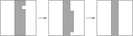
FIG. 16.: Relaxation of a stripe state in two dimensions at small non-zero temperature: (a) Nucleation of a dent; (b) Diffusive growth of the dent; (c) Dent reaches the system size and hence the domain wall steps to the left. This overall process ultimately leads to the disappearance of the stripe.

A stripe is formed in a time of order $L^{2}$[4]. At a small positive temperature, a stripe can disappear by the annihilation of the two domain walls (Fig. 16). This annihilation occurs by the following steps: First, a dent is created by flipping a spin at a domain wall. The time required for this event is of the order of $e^{4J/kT}$, where $4J$ is the energy cost associated with the spin flip. Once a dent is created, the spin in the dent, as well its two vertical neighbors, are now free to flip. Thus the length of the dent performs a one-dimensional random walk until the horizontal boundaries meet.

Now using elementary facts about the first passage of a one-dimensional random walk in the presence of an absorbing boundary[15], the dent recombines with probability $(L-1)/L$ and the domain wall returns to its original state, or with probability $1/L$ the dent expands and changes the sign of one column of spins. Thus we need $L$ dent creation events before the interface of the strip hops rigidly by $\pm 1$ in the $x$-direction. The time needed for this hop is therefore of the order of $L\,\exp(4J/kT)$. Since the typical width of a stripe is of the order of $L$, there must typically be $L^{2}$ such interface hopping events before the two interfaces meet and thus surmount the metastable barrier. As a result, the time for a stripe state to disappear is of the order of $L^{3}\,\exp(4J/kT)$.

Our simulations are in excellent agreement with this prediction for $T/T_{c}\lesssim 0.2$ (Fig. 17). Here the time to reach the equilibrium is defined as the time for the system to first reach the equilibrium value of the magnetization of the Ising model on the square lattice at temperature $T$. This stopping time is dominated by configurations which first reach a stripe state; configurations which relax directly to the equilibrium state reach this state quickly.

FIG. 17.: Time to reach the equilibrium state on the square lattice. The straight line is $L^{3}\,e^{4J/kT}$.

We can develop a similar argument in three dimensions. Since a typical metastable state has the form of two interpenetrating 3-arm stars, let us estimate the time for such a structure to disappear. The lowest energy excitation is to flip a spin in one of the concave corners of this structure (see Fig. 12). This spin flip requires an energy of $4J$ and thus takes a time of the order of $\exp(4J/kT)$. By flipping of the order of $L^{2}$ such spins it is possible to create a planar barrier of one phase which spans the system, at which point the other phase can disappear with no additional energy cost. Since the energy cost associated with the creation of this excitation is $4JL^{2}$, this suggests that the time to surmount the metastable barrier scales as $\exp(4JL^{2}/kT)$, a time which is too long to probe directly by simulations.

V Summary

We have investigated the evolution of a finite Ising system with Glauber kinetics when it is suddenly quenched from infinite to zero temperature. In two dimensions there appears to be a non-zero probability that the system ultimately reaches a frozen metastable state which consists of two or more parallel straight stripes. While our simulations suggest that the probability of reaching a stripe state is positive even as $L\to\infty$, and we have a heuristic argument that $k$-stripe states occur with positive probability for every even $k$, we do not have a rigorous argument to support this observation. This is a fundamental unanswered question.

In three and higher spatial dimensions, the probability that system reaches either the ground state or a frozen state is vanishingly small. Essentially all realizations end up wandering forever on connected iso-energy sets of blinker states. It is easy to visualize these blinkers on a even-coordinated Cayley tree as well as on a small-size cubic lattice. However, we do not have a good way to characterize these blinkers for large finite-dimensional systems. The existence of blinkers means that the kinetic Ising-Glauber system in sufficiently large spatial dimensions belongs to type ${\cal M}$ according to the classification of Newman and Stein[3]. That is, some fraction of the spins flip infinitely often (those on blinkers), while the rest of the spins flip a finite number of times.

One reason for the system not reaching the ground state is that metastable states become more numerous as the spatial dimension increases. The number of these metastable states appears to scale as $\exp({\cal N}^{1-1/d})$ in $d$ dimensions, where ${\cal N}$ is the total number of spins. This makes it plausible that a spin system is more likely to first encounter and get trapped in a metastable state before the ground state can be reached. Associated with the metastable states are a variety of interesting geometric features of the final state, such as the distribution of magnetization and the distribution of energy. Many features of these distributions are still unexplained.

At low temperature, the Ising-Glauber system necessarily reaches equilibrium, but via a two-stage relaxation process. Initially, the kinetics is nearly identical to that of the zero-temperature case. For the subset of systems which reach a metastable stripe state in two dimensions, there is then a slow approach to equilibrium by the nucleation of defects which cause the stripe boundaries to diffuse, ultimately merge, and thus disappear. Because this kinetics is an activated process, the time to relax to equilibrium is extremely slow. Surprisingly, this two-stage picture persists for temperatures up to approximately $0.2T_{c}$ in two dimensions. A similar two-stage picture appears to hold in higher dimensions. However, the time scales associated with surmounting metastable barriers and ultimately reaching the ground state are astronomically long.

We are grateful to NSF grant No. DMR9978902 for partial support of this work.

REFERENCES

- [1] R. J. Glauber, J. Math. Phys. 4, 294 (1963).
- [2] J. D. Gunton, M. San Miguel, and P. S. Sahni in: Phase Transitions and Critical Phenomena, Vol. 8, eds. C. Domb and J. L. Lebowitz (Academic, NY 1983); A. J. Bray, Adv. Phys. 43, 357 (1994).
- [3] C. M. Newman and D. L. Stein, Phys. Rev. Lett. 82, 3944 (1999); Physica A 279, 159 (2000).
- [4] A preliminary account of this work is given in V. Spirin, P. L. Krapivsky, and S. Redner, Phys. Rev. E 63, 036118 (2001).
- [5] See e. g., T. M. Liggett, Interacting Particle Systems (Springer-Verlag, New York, 1985).
- [6] J. Chalupa, P. L. Leath, and G. Reich, J. Phys. C 12, L31 (1979); P. M. Kogut and P. L. Leath, J. Phys. C 14, 3187 (1981); J. Adler, Physica A 171, 453 (1991).
- [7] D. Stauffer and A. Aharony, Introduction to Percolation Theory (Taylor & Francis, London, 1992).
- [8] Anomalies associated with stripes and other metastable states in the Ising model have been hinted at in E. T. Gawlinski, M. Grant, J. D. Gunton, and K. Kaski, Phys. Rev. B 31, 281, (1985); J. Viñals and M. Grant, Phys. Rev. B 36, 7036 (1987); J. Kurchan and L. Laloux, J. Phys. A 29, 1929 (1996); D. S. Fisher, Physica D 102, 204 (1997); A. Lipowski, Physica A 268, 6 (1999). For the Potts model see [9, 10].
- [9] I. M. Lifshitz, Zh. Exp. Theor. Fiz. 42, 1354 (1962) [Sov. Phys.–JETP 15, 939 (1962)].
- [10] S. A. Safran, P. S. Sahni, and G. S. Grest, Phys. Rev. B 28, 2693 (1983); P. S. Sahni, D. J. Srolovitz, G. S. Grest, M. P. Anderson, and S. A. Safran, Phys. Rev. B 28, 2705 (1983).
- [11] P. Sen, Int. J. Mod. Phys. C 8, 229 (1997) and 10, 747 (1999); P. Grassberger and W. Nadler, cond-mat/0010265.
- [12] M. Aizenman, Nucl. Phys. B 485, 551 (1997); J. Cardy, J. Phys. A 31, L105 (1998).
- [13] F. Y. Wu, Rev. Mod. Phys. 54, 235 (1982).
- [14] S. Redner, J. Stat. Phys. 25, 15 (1981).
- [15] S. Redner, A Guide to First-Passage Processes (Cambridge University Press, New York, 2001).