EXCITED STATES OF THE COOPER PROBLEM IN A THREE-DIMENSIONAL DISORDERED SYSTEM

This work presents the study of the excited states of the Cooper problem in the three-dimensional Anderson model. It is shown that the excited pair states remain localized while their excitation energy $\Delta E$ is negative. For $\Delta E>0$ the particles are delocalized over the three-dimensional lattice.

The Cooper problem $\!{}^{{\bf?}}$ is the cornerstone of the well known BCS theory for superconductivity. Even if the Cooper problem deals with only two interacting particles (TIP) above a frozen Fermi sea, it nevertheless captures the essential physical features of the superconducting states. Indeed, in comparison with the BCS theory, the solution of the Cooper problem leads to the appearance of coupled states with a qualitatively correct coupling energy and pair size. Then it seems natural that the study of the Cooper problem with disorder could provide a useful step in the understanding of the superconductivity in presence of relatively strong disorder. The first studies on the Cooper problem with disorder were done for three-dimensional $\!{}^{{\bf?}}$ and two dimensional $\!{}^{{\bf?}}$ systems. These studies $\!{}^{{\bf?},{\bf?}}$ were focused on the properties of the ground state of two particles above a frozen Fermi sea coupled via an on-site attractive Hubbard interaction. This interaction creates a phase of bi-particle localized states (BLS) in the regime of disorder where non-interacting states are delocalized. At the same time the mean-field solution of the Cooper problem (Cooper ansatz) gives delocalized pairs. This shows that the non-diagonal matrix elements of interaction play an important role in presence of disorder. These TIP results are in qualitative agreement with recent many-body investigations $\!{}^{{\bf?},{\bf?}}$ of the ground state of the attractive Hubbard model with disorder.

Here the studies are concentrated on the properties of excited TIP states. For that purpose we introduce the Anderson Hamiltonian for one-particle,

$$H_{1}=\sum_{{\mathbf{n}}}E_{\mathbf{n}}\left\arrowvert{\mathbf{n}}\right\rangle\left\langle{\mathbf{n}}\right\arrowvert+V\sum_{\left\langle{{\mathbf{n,m}}}\right\rangle}\left\arrowvert{\mathbf{n}}\right\rangle\left\langle{\mathbf{m}}\right\arrowvert$$ (1)

where $\mathbf{n}$ and $\mathbf{m}$ are the index vectors on the three-dimensional lattice with periodic conditions, $\left\langle,\right\rangle$ denotes nearest neighbor sites, $V$ is the hopping term and the random on-site energies $E_{\mathbf{n}}$ are homogeneoulsy distributed in the energy interval $\left[-\frac{W}{2},\frac{W}{2}\right]$, where $W$ is the disorder strength. To study the effects of the attractive interaction ($U<0$) on two particles near the Fermi sea we generalize the Cooper approach$\!{}^{{\bf?}}$ for the disordered case. We write the TIP Hamiltonian in the basis of one-particle eigenstates of the Hamiltonian (1). In this basis the Schrödinger equation for TIP reads

$$\left(E_{m_{1}}+E_{m_{2}}\right)\chi^{\lambda}_{m_{1},m_{2}}+U\sum_{m^{\prime}_{1},m^{\prime}_{2}}Q_{m_{1},m_{2},m^{\prime}_{1},m^{\prime}_{2}}\,\chi^{\lambda}_{m^{\prime}_{1},m^{\prime}_{2}}=E_{\lambda}\,\chi^{\lambda}_{m_{1},m_{2}}.$$ (2)

Here $E_{m}$ are the one-particle eigenenergies corresponding to the one-particle eigenstates $\left\arrowvert\phi_{m}\right\rangle$ of $H_{1}$ and $\chi^{\lambda}_{m_{1},m_{2}}$ are the components in the non-interacting eigenbasis $\left\arrowvert\phi_{m_{1}}\otimes\phi_{m_{2}}\right\rangle$ of the $\lambda^{\mbox{\scriptsize th}}$ TIP eigenstate $\left\arrowvert\chi^{\lambda}\right\rangle$ corresponding to the eigenenergy $E_{\lambda}$. The matrix elements $UQ_{m_{1},m_{2},m^{\prime}_{1},m^{\prime}_{2}}$ give the interaction induced transitions between non-interactive eigenstates $\left\arrowvert\phi_{m_{1}}\otimes\phi_{m_{2}}\right\rangle$ and $\left\arrowvert\phi_{m^{\prime}_{1}}\otimes\phi_{m^{\prime}_{2}}\right\rangle$. These matrix elements are obtained by writing the Hubbard interaction in the non-interactive eigenbasis of the model (1). In analogy with the original Cooper problem $\!{}^{{\bf?}}$ the summation in (2) is done over the non-interacting states above the Fermi level, in the labelling $E_{m^{\prime}_{1,2}}>E_{F}$ corresponds to $m^{\prime}_{1,2}>0$. The Fermi energy is determined by a fixed filling factor $\nu=1/2$. To keep similarity with the Cooper problem we restrict the summation on $m^{\prime}_{1,2}$ by the condition $1<m^{\prime}_{1}+m^{\prime}_{2}<M$. In this way the cut-off of M unperturbed orbitals introduces an effective phonon frequency $\omega_{D}\propto M/L^{3}=1/\alpha$ where $L$ is the linear system size. When varying $L$ we keep $\alpha$ fixed so that the phonon frequency is independent of the system size. All the data in this work are obtained with $\alpha=30$ but we also checked that the results are not sensitive to the change of $\alpha$.

In order to analyze the properties of the TIP excited states of the disordered Cooper problem we compute the energy level spacing distribution $P(s)$ obtained by the diagonalization of (2). From $P(s)$ we calculate

$$\eta=\frac{\int_{0}^{s_{0}}\left[P(s)-P_{WD}(s)\right]ds}{\int_{0}^{s_{0}}\left[P_{P}(s)-P_{WD}(s)\right]ds}.$$ (3)

Here $P_{P}(s)=\exp(-s)$ and $P_{WD}(s)=\frac{\pi s}{2}\exp\left(-\frac{\pi s^{2}}{4}\right)$ are respectively the Poisson and the Wigner-Dyson distributions, and $s_{0}\simeq 0.4729$ is their intersection point. In this way, $\eta$ varies from $1$ [$P(s)=P_{P}(s)$] to 0 [$P(s)=P_{WD}(s)$] and thus characterizes a transition from localized to delocalized states. For example for the one-particle problem this method allows to detect efficiently the Anderson transition $\!{}^{{\bf?}}$.

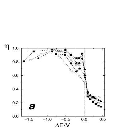
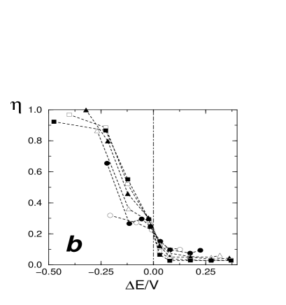
Figure 1: Dependence of $\eta$ on the excitation energy $\Delta E$ for (a) $W=18V>W_{c}\simeq 16.5V$ and (b) $W=12V<W_{c}$. The interaction strength is $U=-4V$ and the linear lattice size is $L=6\,(\circ),7\,(\bullet),8\,(\triangle),10\,(\mbox{full triangle}),12\,(\mbox{square})$ and $14\,(\mbox{full square})$. The number of disorder realization used is $N_{D}=3000$ and $\alpha=30$.

In Fig. 1, $\eta$ is shown for disorder strength $W=18V$ (a) and $W=12V$ (b), an interaction strength $U=-4V$ and for different linear lattice size, from $L=6$ up to $L=14$. $\eta$ is presented versus the excitation energy $\Delta E=E-2E_{F}$ where $E$ is the energy of the two interacting particles. Without interaction for $W=18V>W_{c}\simeq 16.5V$ the one particle states are well localized (see Fig. 2a). When the on-site Hubbard attraction is switched on, coupled states appear below the Fermi energy of two non-interacting particles ($\Delta E<0$). Fig. 1a clearly shows that at the thermodynamic limit the coupled states with $\Delta E<0$ are localized ($\eta\rightarrow 1$). As $W>W_{c}$ all the non-interacting orbitals are localized in the lattice basis. The on-site attractive interaction acts as an additional constraint forcing the two particles (with opposite spin) to stay together in the same well of potential (see Fig. 2b). Above the Fermi energy, $\eta$ tends slowly to 0 indicating that these unbounded states ($\Delta E>0$) are delocalized. This delocalization is due to the fact that an interaction (repulsive or attractive) between particles destroies single particle localization and leads to a propagation of pairs of size $l_{1}$ over a distance $l_{c}$ much larger than $l_{1}$   $\!{}^{{\bf?},{\bf?}}$. The enhancement factor $\kappa$ is then determined by the density $\rho_{2}$ of two-particle states coupled by the interaction and the interaction induced transition rate $\Gamma_{2}$ between noninteracting states, so that $\kappa=\Gamma_{2}\rho_{2}$. For $\Delta E>0$ the density $\rho_{2}$ grows with the excitation energy ($\rho_{2}\propto\Delta E$)$\!{}^{{\bf?}}$ that strongly enhances the delocalization of pairs (see Fig. 2c).

In Fig. 1b, $\eta$ is shown for $W=12V<W_{c}$. For this regime the non-interacting one-particle states are delocalized (see Fig. 2d). For the different linear lattice size $L$ the ground state is still localized ($\eta\simeq 1$) in agreement with $\!{}^{{\bf?}}$. Indeed as $W/W_{c}\simeq 0.72>W_{s}/W_{c}\simeq 0.35$ the TIP ground state is in the BLS phase, where $W_{s}$ is the critical value of the disorder for the superconductor-insulator transition found in $\!{}^{{\bf?}}$ for TIP pairs. In the region $-0.25V<\Delta E<0$ although $\eta$ drops from 0.9 to 0.25 a certain localization of TIP pairs still remains (see Fig. 2e). For $\Delta E>0$, the TIP states become delocalized (see Fig. 2f).

Figure 2: One-particle probability distribution $f_{\lambda}({\mathbf{n}_{1}})=\sum_{{\mathbf{n}_{2}}}\left\arrowvert\chi^{\lambda}_{\mathbf{n_{1},n_{2}}}\right\arrowvert^{2}$ extracted from TIP eigenstates $\left\arrowvert\chi^{\lambda}\right\rangle$ and projected on a (x,y)-plane. The linear lattice size is $L=16$. $f_{\lambda}({\mathbf{n}_{1}})$ is presented for $W=18V$ [ (a) ground state without interaction, (b) excited states $\lambda=25$ with $\Delta E_{\lambda}\simeq-0.25V$ for $U=-4V$ and (c) excited states $\lambda=758$ with $\Delta E_{\lambda}\simeq 0.25V$ for $U=-4V$ ] and for $W=12V$ [ (d) ground state without interaction, (e) excited states $\lambda=83$ with $\Delta E_{\lambda}\simeq-0.05V$ for $U=-4V$ and (f) excited states $\lambda=512$ with $\Delta E_{\lambda}\simeq 0.125V$ for $U=-4V$].

Figure 3: IPR $\xi$ as a function of the coupling energy $\Delta E$ for a disorder strength $W=12\,(\circ)$ [$\Delta E/V$ is then read on the upper horizontal axis] and $W=18\,(\bullet)$ [$\Delta E/V$ is then read on the lower horizontal axis]. The interaction strength is $U=-4V$ and the linear lattice size $L=12$. $N_{D}=300$ disorder realization are used, $\alpha=30$, $2\epsilon\simeq 0.05$ for $W=18$ and $2\epsilon\simeq 0.025$ for $W=12V$.

In order to characterize the wave function properties of the excited states of the disordered Cooper problem, we compute

$$\xi\left(E\right)=\left\langle\left(\sum_{m_{1},m_{2}}\left\arrowvert\chi^{\lambda}_{m_{1},m_{2}}\right\arrowvert^{4}\right)^{-1}\right\rangle_{E_{\lambda}\in\left[E-\epsilon,E+\epsilon\right]}$$ (4)

where the brackets mark the averaging over $N_{D}=400$ realizations of the disorder and over an energy interval $2\epsilon$ centered on $E$. The inverse participation ratio (IPR) $\xi\left(E\right)$ counts the average number of non-interacting states $\left\arrowvert\phi_{m_{1}}\otimes\phi_{m_{2}}\right\rangle$ occupied by the TIP wave functions belonging to energy interval $\left[E-\epsilon,E+\epsilon\right]$. Fig. 3 shows the IPR as a function of the coupling energy $\Delta E$ for $W>W_{c}$ and $W<W_{c}$. For $W=18V$ as the one-particle noninteracting states are localized, only few of these states ($\xi\simeq 5-10$) are enough to build the TIP localized states with $\Delta E<0$. On the contrary for $W=12V$ the TIP localized states ($\Delta E<0$) occupy more noninteracting states ($\xi\simeq 30$) than for $W=18V$ (Fig. 3). Indeed, for $W<W_{c}$ the one-particle noninteracting states are delocalized and it is necessary to have a sufficient number of these states to see the TIP eigenstates localization induced by the quantum interferences.

In conclusion, the study of the excited states of the disordered Cooper problem shows that the BLS phase found in $\!{}^{{\bf?},{\bf?},{\bf?}}$ exists for TIP eigenstates with energy $\Delta E<0$. This phase is destroyed for TIP eigenstates above the Fermi level $\Delta E>0$.

References

References

- [1] L.N. Cooper, Phys. Rev. 104, 1189 (1956).
- [2] J. Lages and D.L. Shepelyansky, Phys. Rev. B 62, 8665 (2000).
- [3] J. Lages and D.L. Shepelyansky, cond-mat/0104194.
- [4] B. Srinivasan and D.L. Shepelyansky, cond-mat/0102055.
- [5] J. Lages, G. Benenti, D.L. Shepelyansky, cond-mat/0101265, to appear in Phys. Rev. B.
- [6] B. I. Shklovskii, B. Shapiro, B. R. Sears, P. Lambrianides and H. B. Shore, Phys. Rev. B 47, 11487 (1993).
- [7] T.Ohtsuki, K.Slevin, T.Kawarabayashi, Ann. Physik (Leipzig) 8, 655 (1999).
- [8] D.L. Shepelyansky, Phys. Rev. Lett. 73, 2607 (1994).
- [9] Y. Imry, Europhys. Lett. 30, 405 (1995).