Macroscopic entanglement in Josephson nanocircuits

Abstract

In this Letter we propose a scheme to generate and detect entanglement between charge states in superconducting nanocircuits. We discuss different procedures to discriminate such entanglement from classical correlations. The case of maximally entangled states of two and three coupled Josephson junctions is discussed as example.

The phenomenon of entanglement, probably one of the most striking feature of quantum mechanics [1], appearing as a consequence of the superposition principle in the presence of composite systems, is the main ingredient in all known examples of quantum speed-up in quantum computation and communication [2, 3]. This has prompted intense experimental efforts towards its generation and detection, most notably with photons [4], cavity QED systems [5], ion traps [6], and coupled quantum dots [7]. Although in condensed matter it is common to encounter correlated many-body states, it is difficult to isolate the different subsystems while maintaining their entanglement. This problem is recently attracting a lot of attention and several solid state devices have been suggested. They are based on the phenomenon of Andreev reflection in hybrid normal-superconducting systems [8, 9] or on the coupling of mesoscopic Josephson junctions with superconducting resonators [10, 11].

In this Letter we propose an explicit experimental scheme to generate and detect entanglement in superconducting nanocircuits. Astonishing progresses have recently been made in the control of the coherent evolution of such systems [12, 13], which have been proposed as promising candidate to realize a quantum computer [14, 15, 16, 17]. In our proposal we specifically address two important issues. i) We describe how to measure the entangled states once the subsystems have been separated and what is the effect of a possible residual coupling on the outcome of the measurements. ii) We show how to distinguish between entangled states and statistical mixtures or product states. Our setup is based on a modification of the device used by Nakamura et al. [13, 18] and, we believe, it is amenable of experimental verification with present days technology.

As sketched in Fig.1, we consider two superconducting Single Electron Tunneling (SET) transistors (labelled by $a,b$) coupled by a small, Josephson junction. By choosing appropriately the working point of the device [13] (see below), coherent Cooper-pair tunneling takes place only across the left and the coupling junctions, while quasi-particle tunneling is important across the right junctions. With these observations the Hamiltonian can be written as a sum of three contributions $H=H_{0}+H_{qp}+H_{T}$. Its coherent part, $H_{0}$, is given by

$$H_{0} = \sum_{i=a,b}\left[E_{ch}(n_{i}-n_{x,i})^{2}-E_{J}\cos 2\varphi_{i}\right]$$ (1)

$$+ E^{(ab)}_{c}(n_{a}-n_{x,a})(n_{b}-n_{x,b})+E_{J}^{(ab)}(\Phi)\cos 2(\varphi_{a}-\varphi_{b})$$ (2)

Here, $E_{ch}$ is the charging energy, $n_{x,i}$ are offset charges induced by external voltages and $E_{J}$ is associated to the Josephson tunneling. The phases $\varphi_{i}$ and the number of charges on the islands $n_{i}$ are conjugate variables $[\varphi_{i},n_{j}]=\,i\;\delta_{ij}$. The state of each individual SET can be manipulated by varying $n_{x}$ with a suitable choice of voltage pulses, for example by putting the left junctions at resonance for Cooper-pair tunneling. However, in order to produce entanglement, we must be able to perform transformations other than local ones. This requires a controllable coupling between the SETs. In our proposal such coupling, $E_{J}^{(ab)}(\Phi)$, is provided by a SQUID, pierced by an external flux $\Phi$. The SQUID capacitance, which we assume to be much smaller than all the other capacitances in the setup, gives rise to an electrostatic coupling, $E^{(ab)}_{c}$. The term $H_{qp}=\sum_{\alpha}\sum_{k\sigma}\varepsilon_{k\alpha}\gamma_{k\sigma\alpha}^{\dagger}\gamma_{k\sigma\alpha}$ ($\alpha=R_{a},R_{b},I_{a},I_{b}$ labels the right electrodes and both islands respectively) describes the quasi-particles. Here, $\gamma_{k\sigma\alpha}^{\dagger}$ ($\gamma_{k\sigma\alpha}$) creates (destroyes) a quasiparticle with momentum $k$ and energy $\varepsilon_{k\alpha}=\sqrt{\xi_{k\alpha}^{2}+\Delta^{2}}$ ($\xi_{k}$ is the single-particle dispersion, $\Delta$ is the superconducting gap and $\sigma$ the spin label). Finally the tunneling Hamiltonian $H_{T}$ is $H_{T}=\sum_{i=a,b}\left[e^{-i\varphi_{i}}\sum_{kq\sigma}T_{kq}\gamma_{k\sigma R_{i}}^{\dagger}\gamma_{q\sigma I_{i}}+h.c.\right]$ where $T_{kq}$ is the amplitude for quasi-particle tunneling. By fixing the transport voltage $|eV|\simeq 2\Delta+E_{ch}$ and due to the Coulomb blockade $E_{ch}\gg E_{J}$, it suffices to consider only three charge states, $n=0,1,2$ and two quasi-particle tunneling rates, $\Gamma_{2}^{a/b}$ and $\Gamma_{1}^{a/b}$. The latter are related to transitions across the right junctions with the charge on the island changing as $n=2\to n=1$ and $n=1\to n=0$ respectively (in the regime we consider, $\Gamma_{2}^{(a/b)}\sim\Gamma_{1}^{(a/b)}\sim\Gamma$ ) [19]. The other tunneling rates are exponentially small. We furthermore assume $\Gamma\ll E_{J}$.

The dynamics of the system can be described by a master equation for the density matrix representing the charge state of the two islands [19]

$$\partial_{t}\rho=i\Bigl{[}\rho,H_{0}\Bigr{]}+\frac{1}{2}\sum_{i=a,b}\sum_{n=1,2}\Gamma_{n}^{(i)}\biggl{\{}2L_{n}^{(i)}\rho\Bigl{(}L_{n}^{(i)}\Bigr{)}^{{\dagger}}-\Bigl{(}L_{n}^{(i)}\Bigr{)}^{{\dagger}}L_{n}^{(i)}\rho-\rho\Bigl{(}L_{n}^{(i)}\Bigr{)}^{{\dagger}}L_{n}^{(i)}\biggr{\}}$$ (3)

where $L_{n}^{(i)}=|n-1\rangle\langle n|_{i}$ is the Lindblad operator corresponding to the quantum jump $n\rightarrow n-1$ for the $i$-th island. The states $|0\rangle$ and $|2\rangle$ of the two SETs are involved in generation of entanglement, while quasi-particle transitions through the states $|1\rangle$ allow to perform the quantum measurement. When such devices are employed as qubits states $|0\rangle$ and $|2\rangle$ are the computational states.

Ideally the detection of entanglement goes through the following steps. i) Prepare the entangled state by means of manipulation of the gate voltages; ii) Switch off the coupling between the two qubits; iii) Perform the measurement.

Preparation - We illustrate one of the possible procedures to prepare the singlet state, $|\Psi^{(-)}\rangle=(|02\rangle-|20\rangle)/\sqrt{2}$. The two junctions are initially kept off degeneracy with the initial state given by $|02\rangle$ . Then, by switching on the Josephson coupling $E_{J}^{(ab)}$, and slightly shifting the working point of the two qubits such that $n_{x,a}-n_{x,b}\simeq E_{J}^{(ab)}/E_{ch}$, for a time $\delta t=\pi/(\sqrt{2}E^{(ab)}_{J})$, the desired singlet state is obtained. In a similar fashion it is possible to generate other maximally entangled states. After the preparation, the coupling between the two SETs should be switched off.

Equally important to the ability to generate entanglement is the possibility to detect it. Below we discuss two possible detection schemes.

Method 1 - The success in the preparation of $|\Psi^{(-)}\rangle$ against decoherence can be tested, as proposed in Ref.[20], by measuring the correlation between the integrated quasiparticle current signals of the two SETs, $\tilde{I}_{a/b}=\int_{0}^{t_{m}}I_{a/b}(t)\,dt$, with the integration time, $t_{m}$, chosen to be much longer than $\Gamma^{-1}$. The correlator is given by ($e$ is the electron charge)

$${\cal C}=e^{-2}\langle\tilde{I}_{a}\tilde{I}_{b}\rangle=e^{-2}\int_{0}^{t_{m}}dt_{1}\-\int_{0}^{t_{m}}dt_{2}\,\langle I_{a}(t_{1})I_{b}(t_{2})\rangle$$ (4)

where the two-time average $\langle I_{a}(t_{1})I_{b}(t_{2})\rangle$ can be obtained with the help of the quantum regression theorem applied to eq. (3). Following the procedure of Nakamura et al. [13], the experiment can be performed by means of repeated preparations of the initial state and measurements of the correlator. A value of ${\cal C}$ different from zero indicates that current is flowing in both channels. This cannot happen if the system is prepared in the $|\Psi^{(-)}\rangle$ state: if island $a$ relaxes from $|2\rangle$ to $|0\rangle$, then $b$ does not and viceversa.

Complete anticorrelation between the two currents is not enough to come to the conclusion that the charge state of the two islands is entangled. A statistical mixture of the form $\rho_{mix}=\frac{1}{2}(|02\rangle\langle 02|+|20\rangle\langle 20|)$ or any convex combination of the kind $\rho_{p}=p\rho_{mix}+(1-p)|\Psi^{(-)}\rangle\langle\Psi^{(-)}|$ would also lead to the same result for ${\cal C}$. In order to discriminate between quantum vs. classical correlations we can proceed in the spirit of experiments testing Bell’s inequality [1]. The basic idea is that if the system is in state $|\Psi^{(-)}\rangle$ the result ${\cal C}=0$ is obtained also if, before the detection stage, one carries out a (further) bi–local unitary operation. For example, one can rotate the state of the two qubits by the same angle $\theta$ bringing both islands to degeneracy for a time interval $\Delta t=2\theta/E_{J}$. This leaves $|\Psi^{(-)}\rangle$ unaffected. On the other hand when the system is in a state like $\rho_{mix}$ bi–local unitary transformations will in general produce a non–zero population in $|22\rangle$ therefore giving rise to a non–zero ${\cal C}$. This is the key ingredient of our scheme to discriminate entangled states from classical mixture.

In the ideal case we can think to switch off the Josephson interaction energy during the measurement, thus ”separating” the two subsystems. If this can be done and if, in addition, also the Josephson energies of the two transistors can be set to zero, then the master equation can be solved exactly. Starting with the state $\rho_{p}$, the integrated current correlation is given by

$${\cal C}_{p}=p\sin^{2}(2\theta)\left[1-e^{-\Gamma t_{m}}-\frac{\Gamma t_{m}}{2}e^{-\Gamma t_{m}}\right]$$ (5)

The two cases of the singlet state and of the complete mixture are obtained for $p=0$ and $1$, respectively. Note that for $p=1$ an oscillatory behaviour is obtained, whose visibility is reduced for $p<1$. Furthermore only when $p=0$ the correlator ${\cal C}$ vanishes.

In order to ascertain the validity of this proposal it is important to check how the residual couplings affect the measurement. Experimentally a non-zero electrostatic coupling will be always present; however, as long as it is small compared to $E_{ch}$, it has no effect on the measurement. More important is the role of $E_{J}$ and of the coupling $E_{J}^{(ab)}$; nevertheless, even if residual Josephson coupling energies are present during the measurement, the singlet and the ] statistical mixture give rise to very different correlation signals. In Figs.2,3 the correlation ${\cal C}$ is shown for $t_{m}=3\Gamma^{-1}$, for both the $p=0$ and $p=1$ cases, and for different values of the charging energy of the SETs and $E_{J}^{(ab)}$, respectively. During the measurement, the Cooper pair states $n=0,2$ should be kept off degeneracy. The amplitude of the oscillations in the mixed case depends on the charging energy $E_{ch}$ (for finite $E_{J}$) because the coherent oscillations in the two SETs may significantly change the state during the measurement. Differences between the pure and mixed state in Fig.2 can be detected down to values of $E_{ch}/E_{J}\geq 1$ (see the dashed line in Fig.2). For lower values of $E_{ch}/E_{J}$, it is impossible to discriminate between the $p=0$ and $p=1$ cases because of the extra Cooper pair tunneling. It is theoretically desiderable and possible experimentally to fix the ratio $E_{ch}/E_{J}\gg 1$, therefore this is not a limitation for the feasibility of our proposal. The signal does not show substantial variations with increasing the Josephson coupling $E_{J}^{(ab)}$ either (see Fig.3). The singlet state always gives rise to a correlation function which does not change with $\theta$. Additional errors, deriving from not perfect gating, are possible; but they are not specific for the measurement of entanglement and it was aready verified [13] that they do not affect the preparation of the state. One can conclude that our proposal is robust against various non-ideal situations that can be encountered in an experiment.

In order to perform current correlation measurements one needs detectors sensitive to single electrons, which is technologically very demanding. One possibility could be to amplify the signals coming from the two qubits before correlating them. A similar procedure has been recently employed to measure the correlation between the two output ports of a fermionic beam splitter [21].

Method 2 - The protocol described so far is particularly suitable to verify that a given maximally entangled state has been created and to detect if decoherence mechanisms have spoiled its coherence. A different approach, which does not require the technologically demanding current correlation measurement (nor an a priori knowledge of which state has to be detected) can be designed as well. The basic requirement of this approach is the ability to implement a two–qubit gate, [22].

To this end we consider the following sequence of voltage pulses. i) Bring the $b$-island to degeneracy with a voltage pulse of duration $t_{1}=\pi/2E_{J}$; ii) Set $n_{x,a}^{-1}=n_{x,b}^{-1}=1+E_{c}^{(ab)}/2E_{ch}$ and let the system evolve for a time $t_{1}=\pi/4E_{c}^{(ab)}$; iii) rotate again the $b$-island of an angle $3\pi/4$ keeping it at degeneracy for a time $t_{3}=3\pi/2E_{J}$. In the computational basis this corresponds to the operation

$${\cal G}=\pmatrix{1&0&0&0\cr 0&1&0&0\cr 0&0&0&-i\cr 0&0&i&0}$$ (6)

which is a C–Not gate apart from a phase factor. It is easy to verify that the deviations from ideal gate operation due to the presence of the electrostatic coupling during single qubit operations are $O(E_{c}^{(ab)}/E_{J})^{2}$. The gate ${\cal G}$ can be used to transform entanglement into coherence of the control qubit, thus providing a mechanism to discriminate entanglement from classical correlations. Indeed we have:

$${\cal G}|\Psi^{(-)}\rangle\langle\Psi^{(-)}|{\cal G} \longrightarrow \frac{1}{2}(|0\rangle-i|2\rangle)(\langle 0|+i\langle 2|)\otimes|2\rangle\langle 2|$$ (7)

$${\cal G}\rho_{mix}{\cal G} \longrightarrow \frac{1}{2}I\otimes|2\rangle\langle 2|$$ (8)

Note that the target qubit ($b$) always factors, while $a$ is left in either a coherent or a completely incoherent superposition of the basis states, depending on the initial presence of entanglement. At this point, one can reveal the coherence of the state of the control qubit by performing a current measurement as in [13]. If the excess current shows oscillations with respect to a varying rotation angle, then the state is coherent and therefore the initial state was a singlet. On the other hand, if the excess current coming from island $a$ is constant one can infer that the initial state was not entangled.

We mention that a Bell state analyzer can be easily implemented with this setup. Indeed by applying ${\cal G}$ followed by a further $\pi/4$ rotation, the four maximally entangled Bell states, $|\Phi^{(\pm)}\rangle=\frac{1}{\sqrt{2}}(|00\rangle\pm|22\rangle)$ and $|\Psi^{(\pm)}\rangle=\frac{1}{\sqrt{2}}(|02\rangle\pm|20\rangle)$, are transformed into the basis state $|20\rangle,|00\rangle,|02\rangle$ and $|22\rangle$, respectively, so that they can be distinguished by two local single-qubit current (or charge) measurements.

All the preceding discussion could have been equally well phrased in terms of charge measurements instead of current ones. In this case, the right junctions are no longer necessary, while the remaining single Cooper pair boxes should be coupled to two electrometers [23] which, in turn, induce a dephasing and a mixing among the qubit states [24]. The procedure can be easily generalized to include more qubits. With a three Josephson qubits setup, GHZ states of the form $\frac{1}{\sqrt{2}}(|000\rangle+e^{i\chi}|222\rangle)$, [25] can be obtained by applying two ${\cal G}$ gates, the first one to $b$ and $a$ and the second one to $b$ and $c$ (with $b$ always as the control qubit).

FIG. 1.: (Top) Schematic representation of the proposed setup. The left junctions and the SQUID allow for the coherent manipulations to prepare the state. The right junctions provide the measurement setup. (Bottom) Procedure to prepare and detect the entanglement. The procedure in repeated as in the experiment in Ref [13]

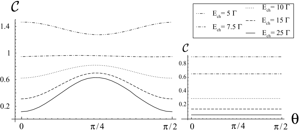
FIG. 2.: Time Average of the current correlation function over the time interval $\Delta t=3\Gamma^{-1}$ as a function of the rotating angle $\theta$ for the case of the mixture (left) and the singlet (right). The parameters in both figures are $E_{J}^{(ab)}=10\Gamma$, $E_{J}=20\Gamma$, $E_{c}^{(ab)}=0.1\Gamma$ and the indicated values for $E_{ch}$.

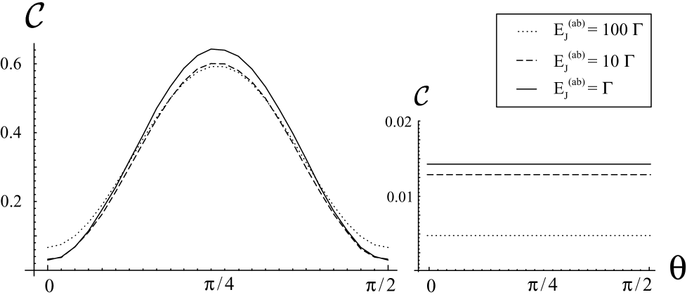
FIG. 3.: The same as in the previous figure, for different values of the Josephson coupling of the SQUID $E_{J}^{(ab)}$ ($E_{ch}=25\Gamma$, $E_{J}=10\Gamma$, $E_{c}^{(ab)}=0.1\Gamma$). The correlator in both cases is almost insesitive to $E_{J}^{(ab)}$

- [1] J.S. Bell, Speakable and unspeakable in Quantum Mechanics, Cambridge University Press (1987).
- [2] A.K. Ekert and R. Jozsa, Phil. Trans. R. Soc. London A, 356,1715, (1998).
- [3] Quantum Computation and Quantum Communication, M.Nielsen and I.Chuang, Cambridge University Press, (2000).
- [4] A. Zeilinger, Rev.Mod.Phys.71, S288,(1999).
- [5] A.Rauschenbeutel, G. Nogues, S. Osnaghi, P. Bertet, M. Brune, J.-M. Raimond, and S. Haroche, Science, 288, 2024, (2000).
- [6] C.A.Sackett, D. Kielpinski, B. E. King, C. Langer, V. Meyer, C. J. Myatt, M. Rowe, Q. A. Turchette, W.M. Itano,D. J. Wineland, and C. Monroe, Nature, 404, 256, (2000)
- [7] M. Bayer, P. Hawrylak, K. Hinzer, S. Fafard, M. Korkusinski, Z. R. Wasilewski, O. Stern, and A. Forchel , Science 291, 451 (2001).
- [8] D. Loss and E.V. Sukhorukov, Phys. Rev. Lett. 84, 1035 (2000); M.-S. Choi, C. Bruder, and D. Loss, Phys. Rev. B 62, 13569 (2000).
- [9] G. B. Lesovik, T. Martin, G. Blatter, cond-mat/0009193.
- [10] O. Buisson, F.W.J. Hekking, cond-mat/0008275
- [11] F. Marquardt and C. Bruder, Phys. Rev. B 63, 054514 (2001).
- [12] V. Bouchiat, D. Vion, P. Joyez, D. Esteve, and M. H. Devoret, Physica Scripta T76, 165 (1998).
- [13] Y. Nakamura, Yu.A. Pashkin, J.S. Tsai, Nature 398, 786 (1999).
- [14] A. Shnirman, G. Schön, and Z. Hermon, Phys. Rev. Lett. 79, 2371 (1997); Y.Makhlin, G.Schön and A.Shnirman, Nature 398, 305 (1999).
- [15] D.A. Averin, Sol. State Comm. 105 659 (1998).
- [16] J.E. Mooij, T.P. Orlando, L. Levitov, L. Tian, C. van der Wal, and S. Lloyd, Science 285, 1036 (1999); L.B. Ioffe, , V.B. Geshkenbein, M.V.Feigel’man, A.L. Fauchere, and G. Blatter,Nature 398, 679 (1999).
- [17] G. Falci, R. Fazio, G.M. Palma, J. Siewert, and V. Vedral, Nature 407, 355 (2000).
- [18] M.-S. Choi, R. Fazio, J. Siewert, and C. Bruder, Europhys. Lett. 53, 251 (2001).
- [19] D. V. Averin and V. Y. Aleshkin, JETP Lett. 50 (7), 367 (1989).
- [20] G. Burkard, D. Loss, E.V. Sukhorukov Phys. Rev. B 61, R16303 (2000).
- [21] M. Henny, S. Oberholzer, C. Strunk, T. Heinzel, K. Ensslin, M. Holland, and C. Schönenberger, Science 284, 296(1999); W.D. Oliver, J. Kim, R.C. Liu, and Y. Yamamoto, Science, 284, 299 (1999).
- [22] In order to implement this second detection strategy, we need , but still .
- [23] R. Schoelkopf, P. Wahlgren, A.A. Kozhevnikov, P. Delsing, and D. E. Prober, Science 280, 1238 (1998)
- [24] Y. Makhlin, G. Schön and A. Shnirman, Phys. Rev. Lett. 85, 4578 (2000).
- [25] D.M. Greenberger, M.A. Horne and A. Zeilinger, Physics Today 46, 22 (1993)