PACS: 75.60.Jp

Abstract

Magnetic properties of 2D systems of magnetic nanoobjects (2D regular lattices of the magnetic nanoparticles or magnetic nanostripes) are considered. The analytical calculation of the hysteresis curve of the system with interaction between nanoobjects is provided. It is shown that during the magnetization reversal system passes through a number of metastable states. The kinetic problem of the magnetization reversal was solved for three models. The following results have been obtained. 1) For 1D system (T=0) with the long-range interaction with the energy proportional to $r^{-p}$, the staircase-like shape of the magnetization curve has self-similar character. The nature of the steps is determined by interplay of the interparticle interaction and coercivity of the single nanoparticle. 2) The influence of the thermal fluctuations on the kinetic process was examined in the framework of the nearest-neighbor interaction model. The thermal fluctuations lead to the additional splitting of the steps on the magnetization curve. 3) The magnetization curve for system with interaction and coercivity dispersion was calculated in mean field approximation. The simple method to experimentally distinguish the influence of interaction and coercivity dispersion on the magnetization curve is suggested.

1 Introduction

The properties of the magnetic nanoobjects and their systems are of current concern due to the appearance of technological possibilities of their fabrication and measurements. The reason of such interest is that such systems are ideal for studying collective effects and phase transitions and are also attractive as a media for high-density magnetic storage. Today there are the experimental data for the magnetization curves of the 2D quadratic lattice of the Ni pillars with the perpendicular anisotropy [1, 2], for the rectangular [3, 4] and square [5, 6] lattices of the permalloy nanoparticles, for the square lattice of CoCrPt particles with the perpendicular anisotropy [7] for the system of the Fe [8] and permalloy [9] nanostripes, for the 2D systems of the chains of the Co particles [10], for anisotropic linear self-assembling mesoscopic Fe particle arrays [11, 12].

What is the main common feature of represented magnetic systems from the theoretical point of view? They consists of the magnetic coercive objects: magnetic particles with the perpendicular single-particle anisotropy [1, 2, 7]; particle chains, which have the effective anisotropy axis along the chain due to interparticle dipole-dipole interaction [3, 10, 11, 12]; magnetic nanostripes having the form anisotropy [8, 9]. In the individual magnetic nanostripe the magnetization process take place by nucleation-propagation process [13, 14]. The propagation of the nucleus is very rapid. The numerical simulation demonstrates, that in 1D nanoparticle chain the magnetization reversal proceeds through nucleation and the following domain wall propagation also [15]. Both magnetic nanostripe and magnetic nanoparticle chain have two stable states within the external magnetic field with the magnetization directed along the stripe or the chain. A nanoparticle with the perpendicular anisotropy axis also has two stable states. The magnetization reversal in the particle has thermoactivated character [16]. In the system of such magnetic nanoobjects there is the long-range interaction between them which have the magnetostatic nature. In systems of the magnetic particles with perpendicular to the array plain anisotropy the interaction has the effective antiferromagnetic character. Its energy

$$E_{ij}=\frac{M(r_{i})M(r_{j})}{|r_{ij}|^{3}},$$ (1)

$M(r_{i})$ is a particle magnetic moment, $r_{ij}$ is interparticle distance. In the case of the system of the magnetic nanostripes the magnetostatic interaction are of long-range character also. It caused by magnetic charges appeared on the stripe edges in the magnetized state. The dependence of the interaction energy on the inter stripe distance is

$$E_{stripe}=2\frac{M(r_{i})M(r_{j})}{L^{2}}(\frac{1}{r_{ij}}-\frac{1}{\sqrt{r_{ij}^{2}+L^{2}}}),$$ (2)

here $M(r_{i})$ is stripe magnetic moment, $r_{i,j}$ is inter stripe distance, $L$ is their length. For the neighboring stripes $E\sim r^{-1}$, on the long distances $E\sim r^{-3}$.

Another system is 2D rectangular lattice of the magnetic nanoparticles with the single-particle anisotropy of the ”easy plain” type. In this case particles form chains lying along the short side of the elementary rectangular. Due to anisotropy character of the dipole interaction the chain magnetization directed along the chain. The energy of the inter chain interaction involves the part (2) connected with the existence of the magnetic charges on the chain edges and the part caused by discreteness nature of the chain [17, 18]:

$$E_{discr}=\frac{8\pi^{2}M(r_{i})M(r_{j})/La^{2}}{\sqrt{r_{ij}/a}}exp(-2\pi r_{ij}/a),$$ (3)

here $M(r_{i})$ is magnetic moment of a chain, $a$ is the interparticle (within chain) distance, $r_{ij}$ is the distance between the chains and $L$ is their length. The relation $E_{discr}/E_{strip}$ is proportional to the chain length. So for the sufficiently long chains the nearest-neighbor interaction plays a leading role [17]. The character of interaction is antiferromagnetic too.

There were made some attempts to solve the problem of the magnetization process in the coercive system with the interaction by numerical methods [19, 20, 21]. It was found, that the magnetization curves look like staircase with the steps of different widths. Besides there is the first report about the experimental observation of such steps [19].

In our work we provide analytical investigation of the problem. In the first part we solve 1D model of system of $2^{N}$ magnetic moments with coercivity and long-range interaction decaying proportionally $1/r^{p}$ which corresponds to the system of magnetic nanostripes. We use the cyclic boundary conditions. It was shown that the magnetization curve consists of the series of steps corresponding to formation of superstructures. In the case $N\rightarrow\infty$ this staircase-like curve has self-similar character (so-called ”devil-staircase”). The method of the solution can be easily generalized on the case of 2D quadratic lattice of the magnetic nanoparticles with perpendicular anisotropy. In second part we solve the problem for 1D system with niarest-neighbor antiferromagnetic interaction and single object coercivity at finite temperature. The influence of thermal fluctuation on the magnetization process described in first part is also discussed here. It is shown that the appearance of defects in the superstructures leads to splitting of the steps on the magnetization curve. The influence of the coercivity dispersion is also discussed. In the third part of the article we use the mean-field approximation to show, how one can distinguish interaction and coercivity dispersion in the system of magnetic nanoobjects. Very easy method to estimate the contribution of interaction and coercivity dispersion in the magnetic properties of the system is suggested.

2 The model with the long range interaction.
”Devil-staircase”

Let us consider the 1D system of long-range interacting coercive magnetic objects. Its appropriate example is system of finite length magnetic nanostripes or chains of magnetic nanoparticles. There is the effective antiferromagnetic interaction of magnetostatic nature between them. We consider its energy in the dimensionless form

$$\epsilon=\frac{I}{|k-n|^{p}}\sigma_{k}\sigma_{n},$$ (4)

here $\sigma_{k}=\pm 1$ are interacting magnetic moments, $n$ and $k$ are the numbers of magnetic moments positions, $I$ is a dimensionless constant of the effective antiferromagnetic interaction ($I>0$). The nearest-neighbor object distance is equal to 1. Let the system is magnetized so, that all $\sigma_{k}=-1$. The magnetization reversal in the totally magnetised system onsets then the field at the object place exceeds its coercivity. In the case of the infinite chain it is

$$H_{1}=H_{c}-2I\xi(p),\qquad\xi(p)=\sum_{k=1}^{N}\frac{1}{k^{p}}.$$ (5)

Here $H_{c}$ is coercivity of the object and it is the same for all objects. The second term is a field originating at the place of one object by all the others.

In a similar way it can be easily calculated, what reversal ends at the external field value

$$H_{2}=H_{c}+2I\xi(p),$$ (6)

when the last object will be reversed. It is interesting to investigate magnetization curve in the region $H_{1}<H<H_{2}$. As the system is one-dimensional, its ground state is disordered. Here we will consider the temperatures less than single object coercivity ($kT<MH_{c}$), so the system can be in a number of metastable states. For example, if the interaction energy in the system is less than energy of coercivity there are $2^{n}$ (n is a number of objects) metastable states at zero external field.

If objects do not have coercivity or temperature of the system is rather high ($kT>>MH_{c}$) system will be in a ground state at any moment. If the external magnetic field is less than $-2I\xi(p)$ or larger then $2I\xi(p)$ the ground state is totally magnetised state. The values of the magnetization of the ground states corresponding to external field at the interval $-2I\xi(p)<H<2I\xi(p)$ can be also found. This thermodynamical problem was solved in [22]. It was obtained that in this case magnetisation curve has steps and looks like self similar ”devil-staircase”.

Here we solve the problem for the case when $kT$ is less than any energy in the system. So system can be in metastable states and the problem of the magnetization reversal can not be solved by thermodynamical methods. We must solve the kinetic problem by correct choice of a consequence of metastable states the system passes through. The problem of such choice become easier in the case when the system consicts of absolutely even number ($N=2^{n}$) of objects and have cyclic boundary conditions.

So the magnetization reversal onsets then the external field exceeds $H_{1}$. Fluctuations are the reason that the place of the first reversed object can be choused arbitrary. Due to antiferromagnetic character of the interaction the additional increase of the external field is necessary to reverse second object. As the interaction decreases with the inter object distance, the second reversed object must be chosen at the largest distance from the first one. It is very easy to choose this place in the case of the system with cyclic boundary conditions (Fig. 1,I).

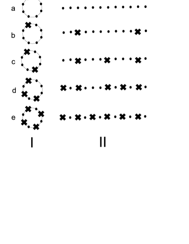
Figure 1: The reversal process in the cyclic system of 8 magnetic moments and corresponding superstructures in the infinite system. Points mark not reversed magnetic moments, crosses mark already reversed ones. The external field increases from a) to e). I) the reversal process in the cyclic system of 8 objects, II) the corresponding superstructures in the infinite system.

In this case the magnetization process takes place through the sequential formation of different superstructures (Fig. 1,II) which are metastable states. Let us calculate the field values, then the definite superstructure appears ($H_{-}$) and became unstable ($H_{+}$). At first we consider only superstructures with period $m=2^{k}$, $k=0,1,2...$ and one reversed object per period (such in Fig. 1 b) c) and e)), $k=0$ corresponds to fully magnetized state. The field, when the superstructure with the period equal to $m$ is formed (Fig. 2), is

$$H_{-}(m)=H_{c}+2I\frac{\xi(p)}{m^{p}}-(2I\xi(p)-2I\frac{\xi(p)}{m^{p}})=H_{c}-2I\xi(p)+4I\frac{\xi(p)}{m^{p}}.$$ (7)

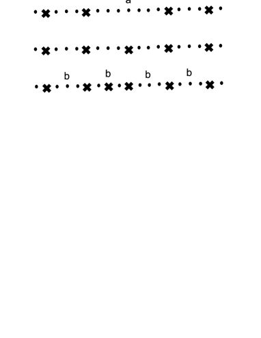
Figure 2: The process of the formation and following destruction of the superstructure with the period $m=4$. Points mark not reversed magnetic moments, crosses mark already reversed ones. $H_{-}$ is the field when the magnetic moment in the point (a) becomes unstable and the formation of the superstructure takes place. $H_{+}$ is the field when the magnetic moments in on of the points (b) become unstable. Due to fluctuations one of them reverses first of all and then prevent others to reverse due to long-range antiferromagnetic interaction.

Here the second term is the fields of already reversed objects. They prevent the chosen object to reverse. The term in brackets is the field of the other not reversed objects. They help chosen object to reverse. In a similar way, the field then the superstructure with the period equal to $m$ become unstable (Fig.2) is

$$H_{+}(m)=H_{c}+2I\frac{(2^{p}-1)\xi(p)}{m^{p}}-(2I\xi(p)-2I\frac{(2^{p}-1)\xi(p)}{m^{p}})$$ (8)

$$=H_{c}-2I\xi(p)+4I\frac{(2^{p}-1)\xi(p)}{m^{p}}.$$

Here we use the relation

$$\sum_{n=1}^{\infty}\frac{1}{(n/2)^{p}}=\sum_{n=1}^{\infty}\frac{1}{(n+1/2)^{p}}+\sum_{n=1}^{\infty}\frac{1}{n^{p}},$$ (9)

The magnetization of the system is determined by the superstructure period and is

$$M=\lim_{N\to\infty}\frac{1}{2^{N}}\sum_{k=1}^{\infty}\sigma_{k}=\frac{2-m}{m}$$ (10)

So there are the mast be steps on the magnetization curves corresponding to the stable superstructures, as the magnetization does not change while the magnetic field changes from $H_{-}(m)$ to $H_{+}(m)$. Using (7,8,10) we can rewrite the dependence of the step edges of the magnetization (Fig. 3) in the form:

$$H_{-}=H_{c}-2I\xi(p)+4I\xi(p)(\frac{M+1}{2})^{p},$$ (11)

$$H_{+}=H_{c}-2I\xi(p)+4I(2^{p}-1)\xi(p)(\frac{M+1}{2})^{p},$$ (12)

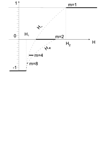
Figure 3: The steps on the magnetization curve corresponding to the simple superstructures ($m=2^{k}$) with one reversed object per period. Magnetization of the corresponding step is $M=(2-m)/m=-1+1/2^{k-1}$

The steps corresponds to the reviewed superstructures do not cover all fields between values $H_{1}$ and $H_{2}$ (Fig. 3). To analyze the magnetization behavior of the system while it transfers from one step to another we must take into account the formation of the more complex superstructures (Fig. 1d). Let us consider, for example, the magnetization process between $H_{+}(m=2)$ and $H_{2}$ (Fig. 3), that is how antiferromagnetic superstructure becomes fully magnetized. The superstructures with periods $m_{2}=2,4...2^{l}$ ($l=1,2...$) appearing with antiferromagnetic ($m_{1}=2$) as a background are represented at Fig.4.

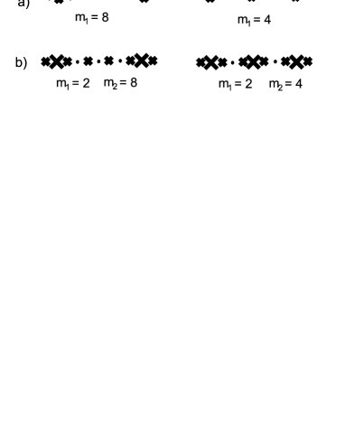
Figure 4: a) are the simple superstructures ($m_{1}$ is a period). Points mark not reversed magnetic moments, crosses mark already reversed ones. b) are complex superstructures characterized by two numbers $m_{1}$ and $m_{2}$. Small crosses mark antiferromagnetic background, big crosses mark reversed magnetic moments forming period of a superstructure.

$m_{1}=2,m_{2}=2$ is totally magnetized state, $m_{1}=2,m_{2}=\infty$ is antiferromagnetic superstructure. In this case $M=2/m_{2}$. The expressions for the magnetic fields $H_{-}(m_{2})$ and $H_{+}(m_{2})$ differ from the case of the simple superstructures as we must take into account the field of the antiferromagnetic background affecting on the objects. This additional field is

$$H=2I\frac{(2^{p}-1)\xi(p)}{m_{1}^{p}}=2I\frac{(2^{p}-1)\xi(p)}{2^{p}}$$ (13)

We must take this field into account twice as formerly it was directed along the external field but now it is directed against it. So we have

$$H_{-}(m_{2})=H_{c}-2I\xi(p)+4I\xi(p)(\frac{M}{2})^{p}+4I\frac{(2^{p}-1)\xi(p)}{2^{p}}$$ (14)

$$H_{+}(m_{2})=H_{c}-2I\xi(p)+4I(2^{p}-1)\xi(p)(\frac{M}{2})^{p}+4I\frac{(2^{p}-1)\xi(p)}{2^{p}}$$ (15)

Evidently (14,15) are exact similar to (11,12), but this curves starts at the point $M=0$, $H=H_{+}(m_{1}=2)=H_{c}-2I\xi(p)+4I\frac{(2^{p}-1)\xi(p)}{2^{p}}$, which is the right edge of the step corresponding to the antiferromagnetic structure, instead of $M=-1$, $H=H_{1}=H_{c}-2I\xi(p)$. In a similar way all other steps on the magnetization curve can be obtained. Each step corresponding to the superstructure is the base of a series of the steps, corresponding to the more complex superstructures with the first one as a background. The dependencies of $H_{-}$ and $H_{+}$ in all cases are similar, and $H_{\pm}\sim M^{p}$. So the picture become self-similar (Fig. 5).

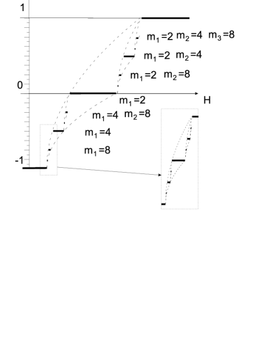
Figure 5: The self-similar ”devil staircase”.

Complex superstructures are characterized by a series of numbers $m_{1},m_{2},m_{3}...$, where $m_{i}=2^{k}$ and $m_{i}<m_{i+1}$. Maximal $m_{max}$ is the period of superstructure, $m_{1},m_{2}...m_{max-1}$ characterizes its background. Narrow steps are between wider ones. Let as find the common width of all steps. The step width can be easily calculated.

$$\Delta H=H_{+}(m)-H_{-}(m)=4I\frac{2^{p}-2}{m_{max}^{p}}\xi(p)$$ (16)

the number of the steps with equal width depends on $m_{max}$ and $N=m_{max}/2$. The common width is

$$\Delta H=\sum_{\mbox{n is even}}^{\infty}N(n)\Delta H(n)=\sum_{\mbox{n is even}}^{\infty}\frac{n}{2}4I\frac{2^{p}-2}{n^{p}}\xi(p)=4I\xi(p)\sum_{k=1}^{\infty}2^{k-1}\frac{2^{p}-2}{2^{kp}}$$ (17)

$$=2I\xi(p)(2^{p}-2)\sum_{k=1}^{\infty}(\frac{1}{2^{p-1}})^{k}=2I\xi(p)(2^{p}-2)\frac{(1/2)^{p-1}}{1-(1/2)^{p-1}}=4I\xi(p)$$

So the sum of all steps widths is exactly the same as the width of the whole inclination of the magnetization curve, which is equal to $4I\xi(p)$ according to (5,6).

The difference in the step width is connected with the decaying character of the long-range interaction. The wider ones are conditioned by interaction of more near magnetic moments; the narrow ones are caused by the interaction of more distant magnetic moments.

The magnetization values corresponding to the steps are

$$M=\frac{4m-1}{m_{max}}-1,$$ (18)

where $m=1,2...m_{max}/2$.

It is interesting, that the exponent in (11) and (12) is equal to the power index in the dependence of the interaction on the inter object distance (4). So it is possible to find the power index for the interaction by the experimental measuring of magnetization curves.

There are some reasons of the distortion of the represented ideal picture. At first it is thermal fluctuations. As for the long distances ($kT>E_{int}(r)$, $k$ is a Boltzman constant) it leads to fuzzifying and disappearing of narrow steps which are conditioned by interaction of distant magnetic moments. Besides thermal fluctuations can lead to appearance of the defects in superstructures. This will be discussed in the next section. The second reason is the bounds of the real system. They can play a significant role as the interaction has a long-range character. Nevertheless if the dimension of the system is larger than $r_{0}$ ($kT=E_{int}(r_{0})$), the influence of the bounds will be neglected by thermal fluctuations. Lastly the dispersion of the objects coercivity can dramatically change the magnetization curve. Such self-similar behavior can be observed only in the system with small (less than interaction) coercivity dispersion. The method how to distinguish the influence of the interaction and coercivity dispersion in possible experiment is discussed in the last section.

In spite of all deficiencies of the proposed model it help to understand the peculiarities of the magnetization process in the system, the nature of the steps on the magnetization curve [19, 21, 23] and especially the fact that the difference in steps width is a sequence of the decaying character long range interaction. It also makes understandable the fact of the alternation of the narrow and wide steps on the magnetization curve [19, 21]. It is very probably that in the general case the magnetization curve has self-similar character too. The model can be easily generalized on the case of the 2D square lattices of the magnetic nanoparticles. In this case one must provide the summation of the dipole sums for the superstructures on the square lattice. The superstructures must have square elementary cell in this case, so the dipole sums can be easy calculated [24].

3 The nearest-neighbor model.
Thermal fluctuations

Let us consider the magnetization process at finite temperature less than the coercive energy of a single magnetic moment $kT<H_{c}M$ but higher than interaction energy of distanced magnetic moments. In this case magnetic moments at distances larger than $r_{0}$ ($kT=E(r_{0})$) begin to reverse independently as their interaction is smaller than the temperature. Nethertheless, as $kT<H_{c}M$ system can be in metastable states. The kinetics of magnetization process can be qualitatively described as follows. When the external magnetic field exceeds the value of $H_{1}$ the thermoactivated reversal of the individual magnetic moments begins. But already reversed magnetic moments prevents neighboring magnetic moments (lying at distances smaller than $r_{0}$) to reverse due to effective antiferromagnetic interaction. More distant magnetic moments can reverse, as the interaction energy in this case is smaller than temperature. Magnetization process has Poisson-like character and ends when the distance between reversed magnetic moments will be in the interval $r_{0}<r<2r_{0}$. The addition external field is necessary to overcome antiferromagnetic interaction and to continue the process of the reverse. Evidently the thermal fluctuations will lead to distortion of the ideal picture described in the previous section. It is difficult to take thermal fluctuations in to account in the general case. Here we have solved the problem for the situation when the temperature is large than any interaction in the system with exception of the most powerful nearest-neighbor interaction. In this case the problem can be solved in the nearest-neighbor approximation ($p=\infty$ in (4)). This model is also appropriate for the case of the planar system of the long chains of the magnetic nanoparticles when the main term in the interaction is interaction of nearest neighbors (3). The form of the hysteresis in this case is represented in Fig.6. The magnetization reversal starts at the field value $H=H_{c}-2I$, as the antiferromagnetic interaction helps the external field.

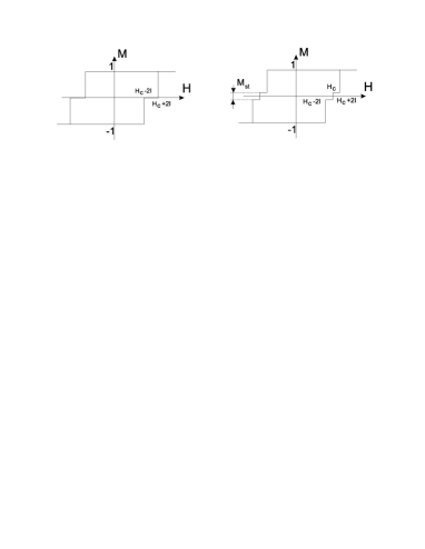
Figure 6: The hysteresis loop in the case of the nearest-neighbor interaction. a) in the case of $T=0$ the step corresponds to antiferromagnetically ordered superstructure. b) the dividing of step in two due to formation of defects in the case of thermal fluctuations. $M_{st}$ is a step high.

The chains begin to reverse the magnetization due to thermal fluctuations. But if the one chain reverses, it prevents the neighboring chains to reverse as the effective field of the interaction is opposite to external field. Due to chaotic character of the sequence of the magnetization reversals of the elements of the system the defects appearances is possible (Fig. 7), and the antiferromagnetic ordering with $M=0$ does not be achieved at this value of the external field. The additional external field ($H=H_{c}$) is necessary to reverse the defects. Then defects change their sign (Fig.7).

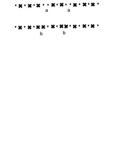
Figure 7: (a) are defects appearing due to Poisson-like character of the magnetization process, (b) are reversed defects. Points mark not reversed magnetic moments, crosses mark already reversed ones.

The magnetization reversal ends within the field $H=H_{c}+2I$ when system becomes totally magnetised. So two steps appear on the each branch of the hysteresis loop. Their width is $\Delta H=2I$ i.e. it depends on the interaction value. The magnetization value $M_{st}$ corresponding to the step depends of defects concentration. It is the special problem to find this concentration. Let us consider the kinetics of the defects appearance in the system of $N$ objects. Firstly all objects are magnetized against external magnetic field $\sigma_{k}=-1$. When the reversal process begins, the reversed objects begin to divide system into the regions of the not reversed objects (we will name them as ”domains”). In process of magnetization the number of domains increases, their widths decrease. Let $P_{n}$ is a number of domains consisted of $n$ not reversed objects then

$$M=\sum_{n=1}^{N-2}P_{n}-\sum_{n=1}^{N-2}nP_{n},$$ (19)

If $\alpha$ is the probability of the chain reverse per unit time, then

$$\frac{\partial P_{n}}{\partial t}=-\alpha(n-2)P_{n}+2\alpha\sum_{k=n+2}^{N}P_{k},\qquad n>2.$$ (20)

The first term is decrease of the domain number due to its dividing into smaller ones; the second term describes the appearance of new domains due to dividing of wider ones. As the domains consisted of one or two objects can not further divide, their number increases only. So

$$\frac{\partial P_{n}}{\partial t}=2\alpha\sum_{k=n+2}^{N}P_{k},\qquad n=1,2.$$ (21)

Evidently $\alpha$ depends on temperature, but as we in the states stable at $t\rightarrow\infty$, $\alpha$ does not affect final result. It can be easily checked, that

$$\frac{\partial}{\partial t}\sum_{n=1}^{N}(n+1)P_{n}=0,$$ (22)

i.e. the whole number of objects in the system is constant. In the course of time ($\alpha t>>1$) only the domains with $n=1,2$ remains. So $P_{n}(t\rightarrow\infty)=0$ for $n>2$ and $M=-P_{2}(t\to\infty)$. Let us use the Laplas transformation and define

$$p_{n}(s)=\int_{0}^{\infty}P_{n}(t)e^{-st}dt.$$ (23)

Then, according to (20)

$$p_{n}(s)=\frac{2\alpha}{\alpha(n-2)+s}Q_{n}(s),$$ (24)

where

$$Q_{n}(s)=\sum_{k=n+2}^{N}p_{k}(s).$$ (25)

For $s\rightarrow 0$

$$Q_{n}(0)=\sum_{k=n+2}^{N}p_{k}(0)=\sum_{k=n+2}^{N}\frac{2}{k-2}Q_{k}(0).$$ (26)

In the recursive form this equation can be written as

$$Q_{n}(0)=Q_{n+1}(0)+\frac{2}{n}Q_{n+2}(0)$$ (27)

To find the magnetization value corresponding to the step it is necessary to calculate $P_{2}(t\rightarrow\infty)$. Evidently

$$P_{2}(t\rightarrow\infty)=\lim_{s\to 0}sp_{2}(s)=2\alpha Q_{2}(0)$$ (28)

If the maximum number of the objects in the system is $N$, $Q_{2}(0)$ can be found from the (27) with the initial conditions $Q_{N-2}=Q_{N-3}=p_{N}(0)$, which are the sequence of (25). In its turn $p_{N}(0)=1/\alpha(N-2)$ according to (20). The solution of the recursive equation was found numerically as

$$M_{st}=2\alpha\lim_{N\to\infty}\frac{Q_{2}(0,N)}{N}\approx 0.134$$ (29)

As $Q_{2}(0,N)$ is proportional to $\alpha^{-1}$, the result does not depend on the value of $\alpha$. So the defects formation during magnetization leads to appearance of two steps on the magnetization curve in the case of the nearest-neighbor interaction. The fluctuational character of the magnetization process prevent chance to find system in the antiferromagnetically ordered ground (if $H=0$) state. One can expect in the case of the long range interaction thermal fluctuations will lead to similar splitting of the magnetization steps too.

4 Dispersion of the coercivity

Another reason of the distortion of the described magnetization process is the dispersion of the coercivity in the system. It is necessary to distinguish the effects of the interaction and the coercivity dispersion especially in experiment. This problem is solved here in the mean field approximation. In the framework of this model the interaction is independent on the distance and $\epsilon=I/N$. It must be mentioned that this model is appropriate in the case of the very long stripes when $L>Na$ ($L$ is a stripe length, $a$ is interstripe distance). The dependence of the magnetization on the external field is linear in this case as

$$H=H_{c}+JM$$ (30)

$H_{c}$ is coercivity, $JM$ is the field of interaction in the mean field approximation. The main feature of the magnetization process in coercive system with the antiferromagnetic interaction is connected with its multistability. It means that if we change the sign of the external field changing the system does not change its magnetization immediately. At first it transits through the whole hysteresis loop from one branch to another (from point A to point B, Fig. 8),

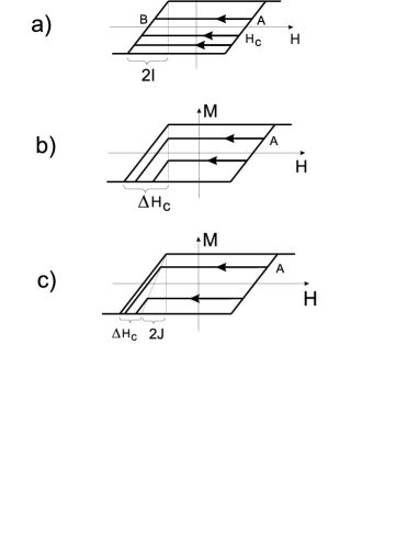
Figure 8: The hysteresis curve in the mean field approximation. a) in the case of the system with interaction. b) in the case of the coercivity dispersion (uniform distribution of the coercivity). c)system both with interaction and coercivity dispersion.

and then begins to change according to the new branch. In this case $|H_{A}-H_{B}|=2H_{c}$. It must be noted that such behavior does not depend on the interaction manner. So different states of the system (characterized by the different magnetization) correspond to the same value of the external field. Such type of the multistability we will name interaction-type (I-type), because the multistability can be in the system of the non-interacting magnetic objects with different values of coercivity also. In this case magnetization reversal begins when field reaches the value $H_{1}=H_{Cmin}$, when the reversal of the objects with the smallest coercivity starts. The reversal process is finished at the field value $H_{2}=H_{Cmax}$, corresponded to the largest coercivity in the system. The hysteresis loop in this case the similar to the one for the system with interaction (as its branches can have similar inclination in the case $\Delta H_{c}=2I$ and uniform distribution of $H_{c}$), but the transitions inside the loop differs. If one change the direction of the reversal process in the A point (Fig.8) in this case, the magnetization does not change while the external field reaches the value of $-H_{1}$ when the reversal of the objects with the smallest coercivity happens. This type of the multistable behavior we will name coercivity-type (C-type). The hysteresis loop of the system both with the interaction and coercivity dispersion can be easily calculated too. It is represented on Fig.8c. So one can distinguish interaction and coercivity dispersion by the behavior of the magnetization within hysteresis loop by analysis of

the multistability type of the system. Evidently the self-similar behavior of the magnetization can be experimentally observed in the systems with small dispersion of coercivity, that is in the systems which demonstrate I-type of multistability. Let us note, that in the reviewed experimental works the type of the multistability is not examined in spite of the simplicity, from the on hand, and, significance, from the other hand, of such investigation.

5 Conclusions

By means of the simple models we have investigated the magnetization processes in the systems of the coercive magnetic objects with interaction. The reason of the formation of the steps on the magnetization curve is investigated. It is shown that the magnetization curve can have self-similar character. Its form is calculated in the case of the long-range interaction with $E\sim 1/r^{p}$. The influence of the thermal fluctuations is analyzed in the framework of the nearest-neighbor approximation. It is shown that fluctuations lead to splitting of the steps on the magnetization curve. The effects of the interaction and coercivity dispersion on the hysteresis loop are examined by mean field approximation. Their difference is shown. It consists in the character of the magnetization dependence on the external magnetic field during the transition between the branches of the hysteresis loop. The understanding of this difference is very important to interpret of the experimental data. It allows to experimentally distinguish the influence of the coercivity dispersion and interaction in the system on the magnetization processes.

References

- [1] M.Hwang, M.C.Abraham, T.A.Savas et al., J. Appl. Phys. 87, 5108 (2000)
- [2] M.Farhoud, H.I.Smith, M.Hwang, C.A.Ross, J. Appl. Phys. 87, 5120 (2000)
- [3] S.A.Gusev, I.M.Nefedov, Yu.N.Nozdrin, et.al., JETP Lett. 68, 509 (1998)
- [4] R.P.Cowburn, A.O.Adeyeye, M.E.Welland, New J. Phys. 1, 16.1 (1999).
- [5] R.P.Cowburn, D.K.Koltsov, A.O.Adeyeye et al., Phys. Rev. Lett. 83, 1042 (1999).
- [6] C.Matheiu, C.Hartmann, M.Bauer et al. Appl. Phys. Lett. 70, 2912 (1997).
- [7] Chiseki Haginoya, Seiji Heike, Masayoshi Ishibashi et al. J. Appl. Phys. 85, 8327 (1999).
- [8] J. Hauschild, H.J. Elmers, U. Gradmann, Phys. Rev. B 57, R677 (1998).
- [9] A.O.Adeyeye, G.Lauhoff, J.A.C.Bland, C.Daboo, D.G.Hasko, H.Ahmed, Appl. Phys. Lett. 70, 1047 (1997).
- [10] J.I.Martin, J.Nogues, Ivan K.Schuller, M.J. Van Bael, K.Temst, C. Van Haesendonck, V.V.Moshchalkov, Y.Bruynseraede,
- [11] Akira Sugawara and M. R. Scheinfein, Phys. Rev. B 56, R8499 (1997).
- [12] Akira Sugawara, G.G.Hembree, M. R. Scheinfein, J. Appl. Phys. 82, 5662 (1997).
- [13] A.Zhukov, M.Vazquez, J.Velazquez et al., J. Magn. Magn. Matt. 170, 323 (1997).
- [14] S.Pignard, G.Goglio, A.Radulescu et al., J. Appl. Phys. 87, 824 (2000).
- [15] A.A.Fraerman, I.M.Nefedov, I.R.Karetnikova et al., Book of abstracts. Moscow International Symposium on Magnetism, MISM99, p.132.
- [16] H.-B. Braun, Phys. Rev. Lett. 71, 3558 (1993).
- [17] M.Gross, S.Kiskamp, Phys. Rev. Lett. 79, 2566 (1997).
- [18] V. M. Rosenbaum, V. M. Ogenko, A. A. Chujko, Usp. Fiz. Nauk, 161, 79 (1991) (in russian).
- [19] D.Grundler, G.Meier, K.-B.Brooks, Ch. Heyn, D.Heitmann, J. Appl. Phys. 85, 6175 (1999)
- [20] J.M.Gonzalez, O.A.Chubykalo, A.Hernando, M.Vazquez, J. Appl. Phys. 83, 7393 (1998)
- [21] G.Brown, M.A.Novotny, Per Arne Rikvold, J. Appl. Phys. 87, 4792 (2000)
- [22] P.Bak, R.Bruinsma, Phys. Rev. Lett., 49, 249(1982)
- [23] L.C.Sampaio, E.H.C.P.Sinnechker, G.R.C.Cernicchiaro et al., Phys. Rev. B 61, 8976 (2000).
- [24] A.A.Fraerman, M.V.Sapozhnikov J. Magn. Magn. Matt. 192, 191 (1999)