Yield conditions for deformation of amorphous polymer glasses

Abstract

Shear yielding of glassy polymers is usually described in terms of the pressure-dependent Tresca or von Mises yield criteria. We test these criteria against molecular dynamics simulations of deformation in amorphous polymer glasses under triaxial loading conditions that are difficult to realize in experiments. Difficulties and ambiguities in extending several standard definitions of the yield point to triaxial loads are described. Two definitions, the maximum and offset octahedral stresses, are then used to evaluate the yield stress for a wide range of model parameters. In all cases, the onset of shear is consistent with the pressure-modified von Mises criterion, and the pressure coefficient is nearly independent of many parameters. Under triaxial tensile loading, the mode of failure changes to cavitation.

I Introduction

The ability to predict the conditions under which a material will yield is of great fundamental interest and technological importance [1, 2, 3, 4]. Over the past three centuries, a number of yield criteria have been formulated that predict whether a combination of stresses on a solid will produce irreversible deformation. In this paper, we use molecular dynamics simulations to test the applicability of these criteria to amorphous polymer glasses under multiaxial loading.

The yield criterion that is most commonly used for polymer glasses is the pressure-modified von Mises (pmvM) criterion. The original von Mises criterion [5] was based on the assumption that yield occurs in the material when the elastic free energy associated with the shear deformation $F_{\rm shear}$ reaches a critical value. For small deformations of an isotropic material, $F_{\rm shear}$ is proportional to the square of the octahedral or deviatoric stress

$$\tau_{\rm oct} = \frac{1}{3}\left((\sigma_{1}-\sigma_{2})^{2}+(\sigma_{2}-\sigma_{3})^{2}+(\sigma_{3}-\sigma_{1})^{2}\right)^{1/2}$$ (1)

$$= \frac{1}{\sqrt{3}}\left((\sigma_{1}+p)^{2}+(\sigma_{2}+p)^{2}+(\sigma_{3}+p)^{2}\right)^{1/2},$$ (2)

where the $\sigma_{i}$ denote the three principal stress components and $p=-(\sigma_{1}+\sigma_{2}+\sigma_{3})/3$ is the hydrostatic pressure. If one ignores anharmonic effects, the condition of yield at constant $F_{\rm shear}$ can be reformulated as yield at a constant threshold value of $\tau_{\rm oct}$, i.e.

$$\tau_{\rm oct}^{y}=\tau_{0}.$$ (3)

For polymers it is often observed [6] that tensile pressure promotes yielding and compressive pressure delays yielding, which is not accounted for in Eq. (3). The pressure modified von Mises criterion [7] includes a linear pressure dependence in the value of the octahedral shear stress at yield,

$$\tau_{oct}^{y}=\tau_{0}+\alpha p.$$ (4)

This pressure modification is motivated by an analogy to friction, where the shear stress is linearly related to normal pressure, rather than to an energy argument like that used to motivate Eq. (3). The coefficient $\alpha$ then plays the role of an internal friction coefficient. Eq. (4) is also employed to describe the shear yield stress in granular materials [8].

The pressure-modified Tresca criterion (pmT) is also often quoted in the context of polymer yielding. Here the relevant quantity is assumed to be the maximum shear stress

$$\tau_{max}=\frac{1}{2}|\sigma_{i}-\sigma_{j}|_{\rm max},$$ (5)

and yield is assumed to occur at

$$\tau_{max}^{y}=\frac{3}{\sqrt{2}}(\tau_{0}+\alpha p).$$ (6)

The prefactor in Eq. (6) is chosen so that, for the same $\tau_{0}$ and $\alpha$, the pmT and pmvM criteria coincide when any two of the three principal stress components are identical. In all other cases, the pmT criterion gives a lower yield stress.

Several experimental studies are available that address the macroscopic yield behavior of polymers. In these experiments, the material is typically strained at a constant strain rate using convenient geometries. The most commonly studied stress states are uniaxial tension or compression, pure shear, and plane strain compression. Several different definitions of the yield point have been employed to determine the yield stress. Most authors [7, 9, 10] take the maximum of the stress-strain curve as the yield stress. The offset-stress [11] is also used, particularly when the stress-strain curve exhibits no clear maximum. It is given by the intersection of the stress-strain curve with a straight line that has the same initial slope as the stress-strain curve but is offset on the strain-axis by a specified strain, e.g. 0.2% (see Figure 2). The offset stress is motivated by the idea that if the load was removed, the sample would relax elastically along the straight line to an unrecoverable strain that is equal to the offset stress. However, the relaxation is generally more complicated. The authors of Ref. [12] argue that the true yield point ought to be determined from the residual strain measured after unloading. They define the yield stress as the smallest stress value that gives a nonzero residual strain.

Raghava et al. [11] collected yield data for polyvinylchloride (PVC), polystyrene (PS), polymethylmethacrylate (PMMA), and polycarbonate (PC). Despite the fact that different definitions of yield were used, all data fit the pmvM criterion[13] with the same value of $\alpha\simeq 0.18$. More recently, Quinson et al. [12] concluded that PMMA is always well described by the pmvM criterion, but that PS follows the pmT criterion at low temperatures and PC always follows the pmT criterion. They associated the validity of the pmT criterion with the occurrence of shear bands. However, Bubeck et al. [10] measured a larger number of yield points for PC and found that they fit the pmvM criterion. This discrepancy may be due to the use of different yield point definitions in the two studies. The small number of uni- and biaxial stress states considered in experimental studies makes it hard to distinguish the two criteria. No experimental tests of yield criteria appear to have considered triaxial stress states.

On the simulation side, both Monte Carlo [14] and Molecular Dynamics simulations [15] have been presented for uniaxial deformation of polymer glasses. Coarse-grained stochastic dynamics of shear flow of local volumes has also been considered [16]. These models were shown to qualitatively reproduce experimental stress-strain curves and their dependence on temperature and strain rate. However, we are unaware of any studies that address multiaxial stress states and relate them to yield criteria.

This paper is organized as follows. In Section II we discuss the details of our model interaction potential for polymer glasses and our method for imposing and measuring stress and strain. Section III begins with a comparison of yield stresses calculated from different definitions of the yield point. We then determine both the maximum stress and the offset stress in multiaxial stress states and compare the results to the pmvM and pmT criteria. In particular, we address the nature of the pressure dependence of the yield stress and investigate the validity of Eqs. (4) and (6) in different physical limits. We conclude with a discussion in Section IV.

II Polymer Model and Simulations

Our model of a polymer glass builds upon extensive simulations of polymer melt dynamics [17]. The solid consists of linear polymers each containing N beads. Pairs of beads of mass $m$, separated by a distance $r$, interact through a truncated Lennard-Jones (LJ) potential of the form

$$V_{\rm LJ}(r) = 4u_{0}\left[(d/r)^{12}-(d/r)^{6}\right]\qquad{\rm for\,\,}r<r_{c}$$ (7)

$$= 0\qquad{\rm for\,\,}r>r_{c},$$ (8)

where $u_{0}$ and $d$ are characteristic energy and length scales. Adjacent beads along the chain are coupled by the FENE potential [17]

$$V_{\rm FENE}(r)=-\frac{1}{2}kR_{0}^{2}\ln[1-(r/R_{0})^{2}]\qquad{\rm for\,\,}r<R_{0},$$ (9)

where $R_{0}=1.5\,d$ and $k=30\,u_{0}/d^{2}$ are canonical choices that yield realistic melt dynamics [18]. Mappings of the potential to typical hydrocarbons [17] give values of $u_{0}$ between 25 and 45 meV and $d$ between 0.5 and 1.3 nm.

The above potentials produce very flexible polymer chains, since no third-, or fourth-body potentials are present. Melt studies of the bead-spring model have recently been extended to include the effect of polymer rigidity [19]. Following these authors, we consider a bond-bending potential for each chain,

$$V_{B}=\sum_{i=2}^{N-1}b\left(1-\frac{(\vec{r}_{i-1}-\vec{r}_{i})\cdot(\vec{r}_{i}-\vec{r}_{i+1})}{|(\vec{r}_{i-1}-\vec{r}_{i})||(\vec{r}_{i}-\vec{r}_{i+1})|}\right),$$ (10)

where $\vec{r}_{i}$ denotes the position of the $i$th bead along the chain, and $b$ characterizes the stiffness.

The equations of motion are integrated using the velocity-Verlet algorithm with a timestep of $dt=0.0075\,\tau_{\rm LJ}$, where $\tau_{\rm LJ}=\sqrt{md^{2}/u_{0}}$ is the characteristic time given by the LJ energy and length scales. Periodic boundary conditions are employed in all directions to eliminate edge effects. We consider two system sizes of 32768 beads and 262144 beads at two temperatures of $T_{\rm h}=0.3\,u_{0}/k_{B}$ and $T_{\rm l}=0.01\,u_{0}/k_{B}$. $T_{\rm h}$ is very close to the glass transition temperature $T_{g}\approx 0.35\,u_{0}/k_{B}$ for this model [20], and $T_{\rm l}$ represents an effectively athermal system. The temperature is controlled with a Nosé-Hoover thermostat (thermostat rate $2\,\tau_{\rm LJ}^{-1}$) [21].

To study the yield behavior, we impose tensile or compressive strains $\epsilon_{i}$ on one or more axes of the initially cubically symmetric solid at constant strain rates of $d\epsilon_{i}/dt=10^{-4}\,\tau_{\rm LJ}^{-1}$ or less. Figure 1 illustrates some of the important limiting stress states that are discussed below. For uni- and biaxial studies of yielding, the stresses $\sigma_{i}$ in the remaining two or one directions are maintained at zero by a Nosé-Hoover barostat (barostat rate $0.1\,\tau_{\rm LJ}^{-1}$) [21]. Note that since $\tau_{\rm LJ}\sim 3\,{\rm ps}$, the strain rates employed are 8-9 orders of magnitude higher than typical experimental strain rates. Nevertheless by comparing to typical sound velocities we can ensure that our strain rates are slow enough that stresses can equilibrate across the system and thus loading proceeds nearly quasistatically. A detailed study of the rate dependence of yielding in polymers will be presented elsewhere.

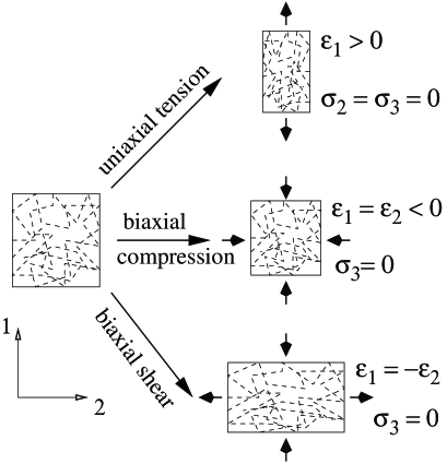
FIG. 1.: Illustration of some limiting stress states employed in this study. For uniaxial simulations $\sigma_{2}$ and $\sigma_{3}$ were kept at zero using a Nosé-Hoover barostat. For biaxial cases $\sigma_{3}$ was kept at zero. The controlled strains were increased at a constant rate.

All stresses in this paper are true stresses, i. e. $\sigma=F/A$, where A is the instantaneous cross-sectional area. Likewise, we use true or logarithmic strains $\epsilon=\int_{l_{0}}^{l}\frac{dl}{l}=\ln(l/l_{0})$. In all cases, stresses are averaged over the entire simulation cell.

Our model lets us address a variety of different physical situations. The influence of adhesive interactions on yielding can be examined by varying the LJ potential cutoff distance from $r_{c}=2^{1/6}\,d$, which gives a purely repulsive interaction, to $r_{c}=1.5\,d$ or $r_{c}=2.2\,d$, which include progressively longer ranges of the attractive tail of the LJ potential. As a byproduct, the density of the solid at zero pressure changes with $r_{c}$.

Polymer dynamics in the melt is greatly influenced by chain length, particularly when entanglements are present. To study the effect of chain length on yielding, we consider an entangled case $N=256\approx 4\times N_{e}$ and an unentangled case $N=16\approx 1/4\times N_{e}$, where $N_{e}\approx 60$ is the entanglement length of the flexible bead-spring model [22]. The bond-bending potential $V_{B}$ is also varied from the flexible limit $(b=0\,u_{0})$ to a semiflexible case $(b=1.5\,u_{0})$.

III Results

A Onset of yielding and yield stress definitions

We begin by considering a uniaxial tension simulation, in which the polymer glass is expanded in one direction, while zero stress is maintained in the perpendicular plane. Figure 2 shows the resulting stress-strain curve. It exhibits the typical features of a polymer glass: linear response is followed by a nonlinear region that bends over into a maximum. Note that the maximum is reached at at strain of about 6%, which is in very good agreement with experimental stress strain curves, see e. g. [12]. Once past that maximum, the stress drops slightly and the material begins to flow, but these large strains are not shown.

FIG. 2.: Stress-strain curve (dashed line) in uniaxial loading. The maximum stress is indicated by $\bullet$ and the 0.2% offset stress by $\blacktriangle$. The latter is determined by the intersection with the straight line, which has the same initial slope as the stress-strain curve, but is displaced by 0.2% on the strain axis. Also shown is the residual strain $\epsilon_{r}$ as a function of the maximum strain during uniaxial ($\square$) or biaxial ($\diamond$) loading. The biaxial results are plotted against the effective strain $\epsilon_{\rm eff}$ (Eq. (11)). Here $T=T_{\rm l},N=256,r_{c}=1.5\,d,b=0\,u_{0},$ and there are 32768 beads.

Fig. 2 also illustrates how to obtain the maximum and offset yield stresses as described in the introduction. Both quantities are easy to identify for uniaxial stress. To make contact with the approach of ref. [12], we have also determined the amount of residual strain after unloading. Squares show the residual strain $\epsilon_{r}$ as a function of the maximum strain before unloading. Results for $\epsilon_{r}>0.2\%$ are comparable to the residual strains given in ref. [12]. These authors identified the yield point with the strain where a linear extrapolation of $\epsilon_{r}$ vanishes. We have extended our studies to much smaller residual strains and find no evidence of a threshold strain below which the residual strain vanishes. Studies of other glassy systems also suggest that at $T=0$ a finite unrecoverable strain should be present for arbitrarily small initial strains, but the theoretical situation at finite $T$ is more complicated [23].

Note that in order to obtain 0.2% residual strain, the initial extension has to be about 4%. This is about twice as large as the yield strain from the 0.2% offset criterion. The offset criterion assumes elastic recovery along the line determined by the elastic moduli of the unperturbed solid. Examination of the recovery curves shows that they are non-linear. This confirms that much of the nonlinear response under loading to the triangle in Fig. 2 is due to recoverable, but anharmonic deformations.

The above discussion raises questions about both the applicability of the unrecoverable strain definition of the yield point and the motivation for the offset stress definition. However, since the offset stress is widely used in engineering applications, we consider both it and the maximum stress definition in the following sections.

B Evaluating the yield stress in multiaxial stress states

Figure 3 shows the principal stress components $\sigma_{i}$ as well as the octahedral shear stress $\tau_{\rm oct}$ for (a) biaxial and (b) triaxial loading. In multiaxial stress states one needs to plot the stress(es) against a scalar effective strain $\epsilon_{\rm eff}$ constructed from the three principal components $\epsilon_{i}$ of the strain tensor. This choice is not unique, and influences the value obtained for the offset stress. A convenient choice that we employ in this paper is

$$\epsilon_{\rm eff}=\frac{1}{\sqrt{2}(1+\nu)}\left((\epsilon_{1}-\epsilon_{2})^{2}+(\epsilon_{2}-\epsilon_{3})^{2}+(\epsilon_{3}-\epsilon_{1})^{2}\right)^{1/2},$$ (11)

where $\nu$ is Poisson’s ratio. This expression is proportional to the octahedral strain and reduces to $\epsilon_{1}$ under uniaxial loading. It also reduces to the effective strain defined in Ref. [11] for biaxial strains, and allows us to treat all strain states on the same footing.

Fig. 3(a) illustrates the maximum and offset definitions of the yield point for biaxial stresses. The maximum of the stress-strain curves is straightforward to evaluate (solid circles), and both nonzero stress components peak at the same strain. By contrast, the offset definition gives yield at slightly different strains (solid triangles). This is troubling, since a yield point should refer to a unique instance in time or strain. Moreover, the offset stress depends on arbitrary factors in the definition of the effective strain and in the amount of offset at the yield point.

We also evaluated the residual strain for different biaxial loading conditions and added them to Fig. 2 (diamonds). Interestingly, these residual strains fall onto the same curve as the results from uniaxial extension when plotted against $\epsilon_{\rm eff}$. As above, there is no indication of a finite threshold below which the residual strain vanishes.

Fig. 3(b) shows that determining the yield point is even more complicated under triaxial loading. For this case, only the tensile stress component exhibits a clear maximum. The compressive components decrease monotonically over the range shown. Moreover, the slope of these curves increases in magnitude with strain so that they do not intersect the line for the offset criterion.

FIG. 3.: Nonzero principal stress components in the model polymer glass during (a) biaxial and (b) triaxial loading. The maximum and offset yield stresses are indicated by $\bullet$ and $\blacktriangle$, respectively. Neither the maximum nor the offset definition can be applied to two of the three components in (b). Also shown is the octahedral shear stress $\tau_{\rm oct}$ (thick dashed line) and the yield stresses that result by applying the yield point definitions to it. Here $T=T_{\rm l},N=256,r_{c}=1.5\,d,b=0$, and there are 32768 beads.

In order to make progress for general multiaxial stress states, we thus decided to apply both the maximum and offset stress definitions not to the three stress components individually, but to the octahedral shear stress $\tau_{\rm oct}$. This is a natural choice given that $\tau_{\rm oct}$ is the quantity that enters the pmvM criterion. The method is illustrated in Fig. 3 and again in Fig. 4, where $\tau_{\rm oct}$ is plotted against the effective strain in a variety of uni-, bi-, and triaxial stress states. For the biaxial states considered in experiments the yield strains obtained from $\sigma_{1}$ and $\sigma_{2}$ separately are nearly the same as that determined from $\tau_{\rm oct}$ [11]. Thus the value of $\tau_{\rm oct}^{y}$ is the same as that constructed from the separate yield components.

In the initial elastic response, stress and strain tensors are linearly related by a combination of the elastic moduli $c_{ij}$ of the solid. The moduli are defined by $c_{ij}\epsilon_{i}=\sigma_{j}$, from which we obtain

$$\tau_{\rm oct}=\frac{\sqrt{2}}{3}\frac{(c_{11}+2c_{12})(c_{11}-c_{12})}{c_{11}+c_{12}}\epsilon_{\rm eff}$$ (12)

by straightforward insertion. Thus a plot of $\tau_{\rm oct}$ versus $\epsilon_{\rm eff}$ should collapse all curves onto a stress-strain curve with common initial slope. Fig. 4 shows that this condition is satisfied for two different temperatures and system sizes. All curves start out with the same slope, but they split apart rapidly at higher strains. This reflects the influence of pressure on yielding. We will show later that this pressure dependence is well described by Eq. (4) for both yield point definitions. As in experiments, the yield stresses decrease with increasing temperature.

FIG. 4.: Octahedral shear stress $\tau_{oct}$ versus effective strain in simulations with (a) 32768 and (b) 262144 beads at $T_{\rm h}=0.3u_{0}/k_{B}$ and $T_{\rm l}=0.01u_{0}/k_{B}$ for different stress states. At low strains, all curves for a given temperature collapse onto a line whose slope is determined by the elastic moduli (Eq. (12)). At higher strains the curves split apart, with the higher curves corresponding to higher pressures. Straight lines are drawn at an offset of 0.2% strain for each temperature. Here $N=256,r_{c}=1.5\,d$, and $b=0\,u_{0}$.

The larger systems in Fig. 4(b) exhibit much smoother curves, since many more independent yield events contribute to the average stress response. However, since the values of yield stress and strain do not change significantly with size, we use systems with 32768 beads in most cases. This speeds up the computations and allows a larger parameter space to be explored. Note that each curve represents the stress response for one particular initial configuration of polymers in the glassy state. We have observed variations on the order of 5% in the magnitude of $\tau_{y}$ with different 32768 bead configurations, but the general features of yielding remained unaltered.

C Biaxial yielding

Experimental tests of yield criteria have generally considered uniaxial or biaxial loading conditions. In the biaxial case, the pmvM criterion predicts that the values of $\sigma_{1}$ and $\sigma_{2}$ at yield should lie on the surface of an ellipse in the $\sigma_{1}-\sigma_{2}$ - plane. The equation for this ellipse can be obtained from Eq. (4) by letting $\sigma_{3}=0$:

$$(\sigma_{1}-\sigma_{2})^{2} + \frac{1-2\alpha}{3}\left(\sigma_{1}+\sigma_{2}+\frac{3\alpha\tau_{0}}{1-2\alpha}\right)^{2}$$ (13)

$$= 6\tau_{0}^{2}\left(1+\frac{\alpha^{2}}{2(1-2\alpha)}\right)$$ (14)

A nonzero value of $\alpha$ breaks the tensile/compressive symmetry and shifts the ellipse towards the lower left quadrant (where the stress is compressive). The amount of the shift increases with $\alpha$. The pmT criterion predicts a yield surface bounded by straight lines. For the same $\tau_{0}$ and $\alpha$, it coincides with the pmvM criterion whenever two of the stresses are equal.

FIG. 5.: Yield points for biaxial stress states. Filled symbols $(\bullet,\blacktriangle)$ correspond to the yield point at $T_{\rm l}$ and open symbols $(\circ,\triangle)$ to $T_{\rm h}$. Circles refer to the maximum yield stress and triangles to the offset-stress. Data in (a) was obtained for 32768 and in (b) for 262144 beads. The ellipses represent the pmvM yield surface, Eq. (13), and the dashed lines show the pmT yield surface. Statistical error bars are indicated by the symbol size. Here $N=256,r_{c}=1.5\,d$, and $b=0\,u_{0}$.

In Fig. 5, we perform an analysis analogous to the experimental studies, where we only include biaxial data from Fig. 4. We employ reflection symmetry about the line $\sigma_{1}=\sigma_{2}$, since the solid is isotropic. We have tested this isotropy in selected cases and find variations on the order of the symbol sizes. The offset stress is generally lower than the maximum stress and becomes very difficult to evaluate at $T_{\rm h}$ due to the small magnitude of the yield stress and the large thermal noise. The yield stresses are larger in the lower left quadrant, indicating that yield is pressure-dependent. Also shown are the yield surfaces predicted by the two yield criteria. As can be seen, the data from both definitions of the yield stress are better described by the pmvM criterion (Eq. (13)) than the pmT criterion. The values of $\tau_{0}$ and $\alpha$ can be found in Table I (see also the next section). In the following discussion we focus on the pmvM criterion, which provides a better fit for all cases studied.

D General stress states

For general stress states it is simplest to test Eq. (4) directly by plotting $\tau_{oct}^{y}$ versus pressure. This plot lets us include triaxial stress states, which could not be discussed in Fig. 5. In Fig. 6(a) we show the maximum shear yield stresses from all stress states at two temperatures. In general one would expect Eq. (4) to hold as long as the mode of failure is shear. The linear law should break down when cavitation occurs in the polymer. Dashed lines in Fig. 6(a) indicate the threshold for cavitation, which only occurs in our model when all three stress components are tensile. For isotropic tensile loading $\tau_{\rm oct}^{y}$ is rigorously zero and can not be used to determine a maximum or offset stress. The endpoint at $\tau_{\rm oct}^{y}=0$ in Fig. 6(a) was determined from the pressure where all three stress components reach a simultaneous maximum. The offset stress is not well-defined in this limit because $\epsilon_{\rm eff}$ also vanishes.

When yield occurs through shear, the yield stresses shown in Fig. 6(a) lie on a straight line as predicted by Eq. (4). To test this linear dependence over a wider range, we have also performed simulations in which the simulation cell was first compressed isotropically to a higher pressure. The same range of strains was then imposed again, and the resulting shear stresses were added to Fig. 6(a). This procedure led to all the points for $p>1.5\,u_{0}/d^{3}$, which lie on the same straight line as data from the uncompressed starting state. Other simulations show that this linearity extends to even greater pressures of up to $20u_{0}/d^{3}$.

Fig. 6(b) shows the offset yield stresses for two temperatures. While, the data from the compressed and uncompressed starting states each fall on a straight line, it is no longer possible to make a common fit through both data sets.

FIG. 6.: Octahedral stress at yield versus pressure at $T_{\rm l}$ (filled symbols) and $T_{\rm h}$ (open symbols). The maximum stress is shown in (a) and the offset stress in (b). Solid lines are fits to Eq. (4), and the values for $\tau_{0}$ and $\alpha$ are given in Table I. Results for $p>1.5\,u_{0}/d^{3}$ were obtained by applying strains to a compressed state (see text). Points where cavitation was observed are connected by a dashed line in (a) and are not shown in (b).

Moreover, the values of $\alpha$ tend to be smaller for the compressed state than the uncompressed state. From Fig. 4 one sees that the value of $\alpha$ from the offset criterion depends on the rate at which stress increases with pressure at fixed strain, and the slope of the stress-strain curve near the intersection. Both factors change with temperature and the choice of offset at yield. For this reason, it is not surprising that values of $\alpha$ from the offset criterion show larger variations than those from determined from the maximum stress.

E Effect of adhesive interactions

Intuitively one would expect that increasing adhesive interactions between polymers would lead to a higher yield stress. In our model this can be achieved by increasing $r_{c}$, which controls how much of the attractive tail in the LJ potential is included. We have verified that increasing $r_{c}$ to $2.2\,d$ produces higher yield stresses and that the yield points are consistent with the pmvM criterion. Biaxial data lie on an ellipse rather than the straight line segments predicted by the pmT criterion (Fig. 5). Values of $\tau_{\rm oct}^{y}$ from general stress states fall onto a straight line when plotted against pressure (see Fig. 7 below) as long as failure occurs through shear rather than cavitation. Fit values of $\tau_{0}$ and $\alpha$ are presented in Table I. The value of $\alpha$ is the same as for smaller $r_{c}$ within our errorbars. The value of $\tau_{0}$ increases, leading to a higher yield stress at all pressures. Increasing $r_{c}$ also suppresses cavitation. The magnitude of the tensile pressure needed to produce cavitation under hydrostatic loading increased by 2 $u_{0}/d^{3}$ at both temperatures.

FIG. 7.: Maximum shear stress $\tau_{\rm oct}^{y}$ minus $\tau_{0}$ at $T_{\rm l}$ (filled symbols) and $T_{\rm h}$ (open symbols) for three different potential cutoffs $r_{c}=1.1225\,d$ $(\bullet,\circ)$, $r_{c}=1.5\,d$ $(\blacktriangle,\triangle)$ and $r_{c}=2.2\,d$ $(\blacktriangledown,\triangledown)$. To avoid overlap, results for $T_{\rm l}$ were displaced vertically by $0.5\,u_{0}/d^{3}$. Points where cavitation occurred are not included in this plot. Solid lines show best fits to all points plotted.

The opposite limit that we can consider is the purely repulsive potential obtained when $r_{c}=2^{1/6}\,d$. Such a solid does not provide any resistance to tensile stresses at $p=0$, but the same range of strains considered above can be applied at higher offset pressures as done in Fig. 6. Once again, the results are in good agreement with the pmvM criterion and values of $\tau_{0}$ and $\alpha$ are quoted in Table I. The value of $\tau_{0}$ is greatly reduced from those for larger $r_{c}$, but $\alpha$ remains unchanged within our errorbars.

To illustrate that $\alpha$ is constant, we summarize data for the maximum shear yield stress as a function of pressure for all three different ranges of the potential in Fig. 7. For each case, the value of $\tau_{0}$ is subtracted, and results for $T_{\rm l}$ are displaced vertically by 0.5 $u_{0}/d^{3}$ in order to avoid overlap with the high temperature data. For each temperature, all of the data points collapse onto a common straight line whose slope is consistent with the independently determined values of $\alpha$. Thus while $\tau_{0}$ decreases rapidly as adhesion is reduced, $\alpha$ remains unchanged. Similar results have been obtained in recent studies [26] of static friction as summarized in Sec. IV.

F Semiflexible and short polymers

In the previous section we showed that the interaction range has a large effect on $\tau_{0}$, but does not significantly alter $\alpha$. Other features of the potential have little effect on either quantity.

We first consider semiflexible polymers with a value of $b=1.5\,u_{0}$ and a cutoff $r_{c}=1.5\,d$ in Eq. (10). This makes the polymer conformation more rigid, and one would therefore expect increased resistance to deformation. Fig. 8 (a) shows that the pmvM criterion also describes yield of this semiflexible polymer. Values of $\tau_{0}$ and $\alpha$ from linear fits in Fig. 8(b) tend to be slightly higher than the values for flexible chains (Table I), but the changes are comparable to statistical uncertainties.

FIG. 8.: Yield points for (a) biaxial stress states and (b) general stress states from simulations with semiflexible chains $(b=1.5\,u_{0})$. As before, filled (open) symbols correspond to $T_{\rm l}$ ($T_{\rm h}$) and circles (triangles) indicate the maximum (offset) yield stress. Solid lines show fits to the pmvM criterion using values of $\alpha$ and $\tau_{0}$ given in Table I. Dashed lines connect points where cavitation occurred. Here $N=256$ and $r_{c}=1.5\,d$ and there are 32768 beads.

Finally, we have considered shorter chains of length $N=16$ to contrast the behavior of unentangled and entangled ($N=256$) chains. The long-range topological properties that are crucial for the dynamics of polymer melts turn out to be irrelevant for the small strains required to initiate yield [24]. Values for $\tau_{0}$ and $\alpha$ do not deviate substantially from the results for $N=256$, and we merely quote them in Table I.

IV Summary and Discussion

We have examined the yield stress of amorphous glassy polymers under multiaxial loading conditions using molecular dynamics simulations. Measurements of the residual strain after unloading indicate that imposing any finite strain produces some permanent plastic deformation. Thus no threshold for the onset of plastic yield could be identified [12]. Two other common definitions of the yield point, the maximum and offset stress, could not be applied separately to the three principal stresses. Instead they were applied to the octahedral shear stress $\tau_{\rm oct}$ for a wide range of loading conditions and model parameters.

In all cases studied, and for both yield definitions, the pressure-modified von Mises criterion provides an adequate description of the shear yield stress. Traditional plots of biaxial yield points are well fit by ellipses (Eq. (13)) and multi-axial results for $\tau_{\rm oct}^{y}$ vary linearly with pressure. The pressure-modified Tresca criterion always shows worse agreement. Although the difference may be small from an engineering perspective ($<21$%), it has implications about the nature of the molecular mechanisms that lead to yield.

More experimental studies seem to be consistent with the pmvM criterion than the pmT criterion, although the number of stress states that has been accessed is relatively small and limited to biaxial cases. One study [12] found that the pmT criterion worked better for polymers that formed shear bands. Shear banding can be influenced by boundary conditions and the method of imposing shear. In particular, our periodic boundary conditions inhibit shear banding and this may be why the pmvM criterion always provided a better fit to the yield stress. It is also possible that the failure criterion is dependent on the specific form of the atomic interactions, and that the simple potentials considered here do not lead to pmT behavior. These will be fruitful subjects for future research.

The dependence of $\tau_{0}$ and $\alpha$ on potential parameters and temperature was explored. The value of $\alpha$ is nearly independent of potential parameters, but seems to increase slightly with increasing temperature. The value from the offset stress is larger and more variable than the value from the maximum stress. The value of $\tau_{0}$ is also relatively insensitive to the chain length $N$ and degree of rigidity, indicating that yield is dominated by local structure. However, $\tau_{0}$ increases rapidly with increases in the attractive interactions between molecules that determine the cohesive energy. The value of $\tau_{0}$ also decreases with increasing temperature. Temperature and rate dependence will be discussed in subsequent work.

Our calculated values of the dimensionless parameter $\alpha$ compare well with typical experimental values. Quinson et al. [12] report values for $\alpha$ between 0.14–0.25 for PMMA, 0.03–0.12 for PC and 0.18–0.39 for PS. As in our simulations, there was a tendency for the value to increase with temperature. Bubeck et al. [10] found values between 0.04–0.07 for PC. Rhagava et al. fit all data for the above polymers and PVC to $\alpha=0.18$, and best fit values for individual polymers ranged from 0.13–0.20. They used the offset stress to determine $\alpha$ and our numbers for this quantity are in the same range: $\alpha=$ 0.11–0.16. Comparing values of $\tau_{0}$ is more complicated because of uncertainty in mapping our potential parameters to specific polymers (see Section II). Using values of $u_{0}$ and $d$ from Ref. [17] our values of $\tau_{0}$ correspond to 1 to 50 MPa. This coincides well with the experimental range [3, 12] of 5–100 MPa, but quantitative comparisons for specific polymers are not possible without more detailed models of atomic interactions.

It is interesting to note a connection between the results reported here and recent studies of the molecular origins of static friction [25, 26]. Macroscopic measurements of the force needed to initiate sliding can be understood as arising from a local yield stress for interfacial shear that rises linearly with normal pressure exactly as in the pmvM criterion (Eq. 4). Moreover, the results presented here parallel results from simulations of the static friction due to thin layers of short chain molecules that are present on any surface exposed to air [26]. These authors find $\tau_{0}$ represents an increase in the effective normal pressure due to adhesive interactions. As in our study, $\tau_{0}$ increases with the range of interactions, $r_{c}$, and the value of $\alpha$ is insensitive to many details of the interactions. A simple geometrical model for $\alpha$ was developed based on the idea that surfaces must lift up over each other to allow interfacial sliding. It will be interesting to determine whether a similar geometric model can be developed for yield of bulk polymers.

TABLE I.: Values for $\tau_{0}$ and $\alpha$ obtained from the linear fits in Figures 6, 8 as well as the simulations with $r_{c}=2.2\,d$. Unless otherwise noted, $N=256$ and $b=0$. Typical statistical errors in fits for the maximum yield stress are $\pm 0.02\,u_{0}/d^{3}$ for $\tau_{0}$ and $\pm 0.01$ for $\alpha$. Errors are about three times larger for $\tau_{0}$ in the purely repulsive case, and for all offset stress results.

	$T_{\rm l}$ max	$T_{\rm l}$ offset	$T_{\rm h}$ max	$T_{\rm h}$ offset
	$\tau_{0}/\alpha$	$\tau_{0}/\alpha$	$\tau_{0}/\alpha$	$\tau_{0}/\alpha$
$r_{c}=2^{1/6}\,d$	$0.06/0.08$	—	$-0.42/0.09$	—
$r_{c}=1.5\,d$	$0.72/0.08$	$0.37/0.15$	$0.23/0.10$	$0.11/0.16$
$r_{c}=1.5\,d$, comp.	$0.72/0.08$	$0.24/0.11$	$0.23/0.10$	$0.15/0.06$
$r_{c}=2.2\,d$	$0.83/0.09$	$0.53/0.16$	$0.45/0.10$	$0.28/0.09$
$r_{c}=1.5\,d,b=1.5$	$0.76/0.10$	$0.44/0.13$	$0.31/0.15$	$0.19/0.11$
$r_{c}=1.5\,d,N=16$	$0.68/0.07$	$0.36/0.14$	$0.20/0.12$	$0.07/0.06$