Extremal Optimization for Graph Partitioning

Abstract

Extremal optimization is a new general-purpose method for approximating solutions to hard optimization problems. We study the method in detail by way of the NP-hard graph partitioning problem. We discuss the scaling behavior of extremal optimization, focusing on the convergence of the average run as a function of runtime and system size. The method has a single free parameter, which we determine numerically and justify using a simple argument. Our numerical results demonstrate that on random graphs, extremal optimization maintains consistent accuracy for increasing system sizes, with an approximation error decreasing over runtime roughly as a power law $t^{-0.4}$. On geometrically structured graphs, the scaling of results from the average run suggests that these are far from optimal, with large fluctuations between individual trials. But when only the best runs are considered, results consistent with theoretical arguments are recovered. PACS number(s): 02.60.Pn, 05.65.+b, 75.10.Nr, 64.60.Cn.

I Introduction

Optimizing a system of many variables with respect to some cost function is a task frequently encountered in physics. The determination of ground-state configurations in disordered materials MPV ; Grest ; D+S ; Disorder and of fast-folding protein conformations Proteins are but two examples. In cases where the relation between individual components of the system is frustrated Toulouse , the cost function often exhibits a complex “landscape” cnls in configuration space, posing challenges to neighborhood search procedures. Indeed, for growing system size the cost function may exhibit a rapidly increasing number of unrelated local extrema, separated by sizable barriers that can make the search for the exact optimal solution unreasonably costly. It is of great importance to develop fast and reliable approximation methods for finding optimal or acceptable near-optimal solutions with high probability.

In recent papers we have introduced a new method, called extremal optimization (EO), to tackle such hard optimization problems BoPe1 ; GECCO . EO is a method based on the dynamics of non-equilibrium processes and in particular those exhibiting self-organized criticality BTW , where better solutions emerge dynamically without the need for parameter tuning. Previously, we have discussed the basic EO algorithm, its origin, and its performance compared with other methods. We have demonstrated that the algorithm can be adapted to a wide variety of NP-hard problems PPSN_CISE . We have shown that for the graph partitioning problem, a simple implementation of EO yields state-of-the-art solutions, even for systems of $N>10^{5}$ variables BoPe1 . For large graphs of low connectivity, EO has been shown to be faster than genetic algorithms Holland and more accurate than simulated annealing Science , two other widely applied methods. A numerical study EOperc has shown that EO’s performance relative to simulated annealing is particularly strong in the neighborhood of phase transitions, “where the really hard problems are” Cheeseman . In fact, preliminary studies of the phase transition in the 3-coloring problem PT3COL as well as studies of ground state configurations in spin glasses EO_PRL ; D+S suggest that EO may become a useful tool in the exploration of low-temperature properties of disordered systems.

In the present work we focus on the intrinsic features of the method, by investigating its average performance. For this purpose, we have performed an extensive numerical study of EO on the graph bipartitioning problem. We have considered various kinds of graph ensembles, both with geometric and with random structure, for an increasing number of vertices $N$. The results show that for random graphs, EO converges towards the optimal configuration in a power-law manner, typically requiring no more than $O(N)$ update steps. For geometric graphs the averaged large-$N$ results are less convincing, but if we instead focus on the best out of several trials, near-optimal results emerge. Our implementation of EO has one single tunable parameter, and we find a simple relation to estimate that parameter given the allowed runtime and system size. Many of our numerical results here have been independently confirmed by J. Dall Dall .

The paper is organized as follows. In Sec. II we introduce the graph bipartitioning problem, and in Sec. III we describe the extremal optimization algorithm. Sec. IV deals in detail with our numerical results. In Sec. V we conclude with an outlook on future work.

II Graph Bipartitioning

II.1 Definition

The graph bipartitioning problem (GBP) is easy to formulate. Take $N$ vertices, where $N$ is an even number, and where certain of the vertex pairs are connected by an edge. Then divide the vertices into two sets of equal measure $N/2$ such that the number of edges connecting both sets, the “cutsize” $m$, is minimized. The global constraint of an equal division of vertices places the GBP among the hardest problems in combinatorial optimization, since determining the exact solution with certainty would in general require a computational effort growing faster than any power of $N$ NP_Hard . It is thus important to find “heuristic” methods that can obtain good approximate solutions in polynomial time. Typical examples of applications of graph partitioning are the design of integrated circuits (VLSI) A+K and the partitioning of sparse matrices HL .

The general description of a graph in the previous paragraph is usually cast in more specific terms, defining an ensemble of graphs with certain characteristic. These characteristics can affect the optimization problem drastically, and often reflect real-world desiderata such as the geometric lay-out of circuits or the random interconnections in matrices. Therefore, let us consider a variety of different graph ensembles, some random and some geometric in structure.

II.2 Classes of graphs studied

One class of graphs that has been studied extensively is that of random graphs without geometric structure RandGraph . Here, edges between any two vertices are taken to exist with probability $p$: on the average, an instance has a total of $E=pN(N-1)/2$ vertices and the mean connectivity per vertex is $\alpha=p(N-1)$. Following standard terminology we refer to graphs of this sort as the ensemble of random graphs, even though the other classes of graphs we consider all have stochastic properties as well.

Another often-studied class of graphs without geometric structure is generated by fixing the number of connections $\alpha$ at each vertex, but with random connections between these vertices W+S ; Banavar . In particular, we consider here the case where $\alpha=3$: the ensemble of trivalent graphs, randomly connected graphs with exactly three edges originating from each vertex.

The third class we consider is an ensemble with geometric structure, where the vertices are situated on a cubic lattice. Edges are placed so as to connect some (but not all) nearest neighbors on the lattice: a ratio $x$ of the total number of nearest-neighboring pairs are occupied by an edge, and those edges are distributed at random over the possible pairs. For a cubic lattice, the average connectivity is then given by $\alpha=6x$. This class of graphs corresponds to a dilute ferromagnet, where each lattice site holds a $\pm$-spin and some (but not all) nearest-neighboring spins possess a coupling of unit strength. Here, the GBP amounts to the equal partitioning of $+$ and $-$ spins while minimizing the interface between the two types M+P , or simply finding the ground state under fixed (zero) magnetization. We thus refer to this class as the ensemble of ferromagnetic graphs.

The final class we consider is that of geometric graphs specified by $N$ randomly distributed vertices in the 2-dimensional unit square, where we place edges between all pairs whose two vertices are separated by a distance of no more than $d$ JohnsonGBP . The average connectivity is then given by $\alpha=N\pi d^{2}$. The GBP on this class of graphs has the advantage of a simple visual representation, shown in Fig. 1. Again following standard terminology, we refer to this class simply as the ensemble of geometric graphs.

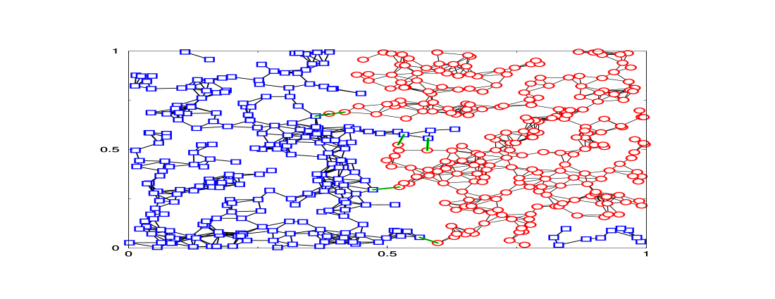
Figure 1: Plot of a geometric graph with $N=500$ vertices and average connectivity $\alpha=6$, partitioned into 250 red and 250 blue vertices. Starting from an initial random assignment of red and blue colors, EO arrives at near-optimal configurations consisting of domains of red and blue vertices, separated by an interface across which “bad” edges (green lines) connect poorly-adapted vertices.

It is known that graphs without geometric structure, such as those in the first two classes, are typically easier to optimize than those with geometric structure, such as those in the final two classes JohnsonGBP . The characteristics of the GBP for non-geometric and geometric graphs at low connectivity appear to be very different, due to the dominance of long loops in the former and short loops in the latter. The ensemble of random graphs has a structure that is locally tree-like, allowing for a mean-field treatment that yields some exact results M+P . By contrast, the ensemble of geometric graphs corresponds to continuum percolation of “soft” (overlapping) circles, for which precise numerical results exist Balberg .

Each of the graph ensembles that we consider is characterized by a control parameter, the average connectivity $\alpha$. The difficulty of the optimization problem for each type varies significantly with $\alpha$. In this study we focus on sparse graphs for which $\alpha$ is kept constant, independent of $N$. Sparse graphs have very different properties from the dense graphs studied by Fu and Anderson F+A . These sparse graphs are generally considered to pose the most difficult partitioning problems, and extremal optimization (EO) is particularly competitive in this regime EOperc . In order to facilitate our average performance study, we fix $\alpha$ to a given value on each ensemble. For random graphs, where the connectivity varies between vertices according to a Poisson distribution, let $\alpha=p(N-1)=2$ (and so $p\sim 1/N$). For trivalent graphs, by construction $\alpha=3$. For ferromagnetic graphs, let $\alpha=6x=2$. For geometric graphs, let $\alpha=N\pi d^{2}=6$. In all of these cases, the connectivity is chosen to be just above the phase transition at $\alpha_{\rm crit}$, below which the cutsize $m$ almost always vanishes EOperc . These critical regions are especially interesting because they have been conjectured to coincide with the hardest-to-solve instances in many combinatorial optimization problems Cheeseman ; PhaseTrans .

Finally, in light of the numerous comparisons in the physics literature between the GBP and the problem of finding ground states of spin glasses MPV , it is important to point out the main difference. This is highlighted by the ensemble of ferromagnetic graphs. Since couplings between spins are purely ferromagnetic, all connected spins invariably would like to be in the same state; there is no possibility of local frustration. Frustration in the GBP merely arises from the global constraint of an equal partition, forcing spins along an interface to attain an unfavorable state (see Fig. 1). All other spins reside in bulk regions where they can maintain the same state as their neighbors. In a spin glass, on the other hand, couplings can be both ferromagnetic and anti-ferromagnetic. Spins everywhere have to compromise according to conflicting conditions imposed by their neighbors; frustration is local rather than global.

II.3 Basic scaling arguments

If we neglect the fact that the structure of these sparse graphs is that of percolation clusters, we can obtain some elementary insights into the expected scaling behavior of the optimal cutsize with increasing size $N$, $m\sim N^{1/\nu}$. For graphs without geometric structure (random graph ensemble and trivalent graph ensemble), one can expect that the cutsize should grow linearly in $N$, i.e., $\nu=1$. Indeed, this argument can be made rigorous for arbitrary connectivity $\alpha$. Extremal optimization performs very well on these graphs, and previous numerical studies using EO all give $\nu\approx 1$ EOperc .

For graphs with geometric structure (ferromagnetic graph ensemble and geometric graph ensemble), the value of $\nu$ is less clear. We can approximate a graph with a $d$-dimensional geometric structure as a hyper-cubic lattice of length $L=N^{1/d}$, where the lattice sites are the vertices of the graph and the nearest-neighbor bonds are the edges, of which only a finite fraction are occupied. There are thus about $E\sim N$ edges in the graph. To partition the graph, we are roughly looking for a $(d-1)$-dimensional hyper-plane cutting the graph into two equal-sized sets of vertices. Such an interface between the partitions would cut $\sim L^{d-1}$ bonds, and thus $\sim N^{1-1/d}$ edges. Following this argument, the 3-d ferromagnetic graphs should have a cutsize scaling with $N^{2/3}$ and the 2-d geometric graphs should have a cutsize scaling with $N^{1/2}$.

However, while this may the case for a typical partition of the graph, it may not be the case for an optimal partition. The interface for an optimal cut of a sparse graph could well be much rougher than our argument suggests, taking advantage of large voids between clusters of connected vertices. The number of cut edges would then be much below the estimate based on assuming a flat interface, making $1/\nu<1-1/d$. In our previous studies using EO, we found $1/\nu\approx 0.75\pm 0.05$ for ferromagnetic graphs and $1/\nu\approx 0.6\pm 0.1$ for geometric graphs EOperc , i.e., above the upper bound, and our newer results do not improve on these (seen later in Fig. 6). This could indicate that the actual values are close to the upper bound, but also that for graphs with geometric structure EO fails to find the optima on instances of increasing size.

Similar behavior has been observed with other local search methods JohnsonGBP , reflecting the fact that sparse geometric graphs generally pose a much greater challenge than do sparse random graphs. In contrast, a heuristic such as METIS METIS , a hierarchical decomposition scheme for partitioning problems, works better for geometric graphs than for random graphs unpublished . METIS performs particularly well for sparse geometric graphs, and typically produces better results than EO for $\alpha=6$. Furthermore, if speed is the dominant requirement, METIS is superior to any local search method by at least a factor of $N$. But for random graphs at $\alpha=2$ or the trivalent graphs, METIS’ results are poor compared to EO’s, and for all type of graphs METIS’ performance deteriorates with increasing connectivity.

III Extremal Optimization Algorithm

III.1 Motivation

The extremal optimization method originates from insights into the dynamics of non-equilibrium critical phenomena. In particular, it is modeled after the Bak-Sneppen mechanism BS , which was introduced to describe the dynamics of co-evolving species.

Species in the Bak-Sneppen model are located on the sites of a lattice, and each one has a “fitness” represented by a value between 0 and 1. At each update step, the smallest value (representing the most poorly adapted species) is discarded and replaced by a new value drawn randomly from a flat distribution on $[0,1]$. Without any interactions, all the fitnesses in the system would eventually approach 1. But obvious interdependencies between species provide constraints for balancing the system’s overall condition with that of its members: the change in fitness of one species impacts the fitness of an interrelated species. Therefore, at each update step, the Bak-Sneppen model replaces the fitness values on the sites neighboring the smallest value with new random numbers as well. No explicit definition is provided for the mechanism by which these neighboring species are related. Yet after a certain number of updates, the system organizes itself into a highly correlated state known as self-organized criticality (SOC) BTW . In that state, almost all species have reached a fitness above a certain threshold. But these species merely possess what is called punctuated equilibrium G+E : since only one’s weakened neighbor can undermine one’s own fitness, long periods of “stasis”, with a fitness above the threshold, are inevitably punctuated by bursts of activity. This co-evolutionary activity cascades in a chain reaction (“avalanche”) through the system. These fluctuations can involve any number of species, up to the system size, making any possible configuration accessible. Due to the extremal nature of the update, however, the system as a whole will always return to states in which practically all species are above threshold.

In the Bak-Sneppen model, the high degree of adaptation of most species is obtained by the elimination of poorly adapted ones rather than by a particular “engineering” of better ones. While such dynamics might not lead to as optimal a solution as could be engineered under specific circumstances, it provides near-optimal solutions with a high degree of latency for a rapid adaptation response to changes in the resources that drive the system. A similar mechanism, based on the Bak-Sneppen model, has recently been proposed to describe adaptive learning in the brain C+B .

III.2 Algorithm description

Inspired by the Bak-Sneppen mechanism, we have devised the EO algorithm with the goal of accessing near-optimal configurations for hard optimization problems using a minimum of external control. Previously, we have demonstrated that the EO algorithm is applicable to a wide variety of problems EO_PRL ; PPSN_CISE . Here, we focus on its implementation for the GBP.

In the GBP, EO BoPe1 considers each vertex of a graph as an individual variable with its own fitness parameter. It assigns to each vertex $i$ a “fitness”

$$\lambda_{i}=g_{i}/(g_{i}+b_{i}),$$ (1)

where $g_{i}$ is the number of “good” edges connecting $i$ to other vertices within its same set, and $b_{i}$ is the number of and “bad” edges connecting $i$ to vertices across the partition. (For unconnected vertices we fix $\lambda_{i}=1$.) Note that vertex $i$ has an individual connectivity of $\alpha_{i}=g_{i}+b_{i}$, while the overall mean connectivity of a graph is given by $\alpha=\sum_{i}\alpha_{i}/N$ and the cutsize of a configuration is given by $m=\sum_{i}b_{i}/2$.

At all times an ordered list is maintained, in the form of a permutation $\Pi$ of the vertex labels $i$ such that

$$\lambda_{\Pi(1)}\leq\lambda_{\Pi(2)}\leq\ldots\leq\lambda_{\Pi(N)},$$ (2)

and $i=\Pi(k)$ is the label of the $k$th ranked vertex in the list.

Feasible configurations have $N/2$ vertices in one set and $N/2$ in the other. To define a local search of the configuration space, we must define a “neighborhood” for each configuration within this space Reeves . The simplest such neighborhood for the GBP is given by an exchange of (any) two spins between the sets. With this exchange at each update we can search the configuration space by moving from the current configuration to a neighboring one. In close analogy with the Bak-Sneppen mechanism, our original parameter-free implementation of EO merely swapped the vertex with the worst fitness, $\Pi(1)$, with a random vertex from the opposite set BoPe1 . Over the course of a run with $t_{\rm max}$ update steps, the cutsize of the configurations explored varies widely, since each update can result in better or worse fitnesses. Proceeding as with the gap-equation in the Bak-Sneppen model PMB , we can define a function $m(t)$ to be to be the cutsize of the best configuration seen during this run up to time $t$. By construction $m(t)$ is monotonically decreasing, and $m(t_{\rm max})$ is the output of a single run of the EO-algorithm.

We find that somewhat improved results are obtained with the following one-parameter implementation of EO. Draw two integers, $1\leq k_{1},k_{2}\leq N$, from a probability distribution

$$P(k)\propto k^{-\tau},\quad(1\leq k\leq N),$$ (3)

on each update, for some $\tau$. Then pick the vertices $i_{1}=\Pi(k_{1})$ and $i_{2}=\Pi(k_{2})$ from the rank-ordered list of fitnesses in Eq. (2). (We repeatedly draw $k_{2}$ until we obtain a vertex in the opposite set from $k_{1}$.) Let vertices $i_{1}$ and $i_{2}$ exchange sets no matter what the resulting new cutsize may be. Then, reevaluate the fitnesses $\lambda$ for $i_{1}$, $i_{2}$, and all vertices they are connected to ($2\alpha$ on average). Finally, reorder the ranked list of $\lambda$’s according to Eq. (2), and start the process over again. Repeat this procedure for a number of update steps per run that is linear in system size, $t_{\rm max}=AN$, and store the best result generated along the way. Note that no scales to limit fluctuations are introduced into the process, since the selection follows the scale-free power-law distribution $P(k)$ in Eq. (3) and since — unlike in heat bath methods — all moves are accepted. Instead of a global cost function, the rank-ordered list of fitnesses provides the information about optimal configurations. This information emerges in a self-organized manner merely by selecting with a bias against badly adapted vertices, rather than ever “breeding” better ones.

III.3 Discussion

III.3.1 Definition of fitness

We now discuss some of the finer details of the algorithm. First of all, we stress that we use the term “fitness” in the sense of the Bak-Sneppen model, in marked contrast to its meaning in genetic algorithms. Genetic algorithms consider a population of configurations and assign a fitness value to an entire configuration. EO works with only a single configuration and makes local updates to individual variables within that configuration. Thus, it is important to reiterate that EO assigns a fitness $\lambda_{i}$ to each of the system’s $N$ variables, rather than to the system as a whole.

While the definition of fitness in Eq. (1) for the graph partitioning problem seems natural, it is by no means unique. In fact, in general the sum of the fitnesses does not even represent the cost function we set out to optimize, because each fitness is locally normalized by the total number of edges touching that vertex. It may seem more appropriate to define fitness instead as $\lambda_{i}=g_{i}$, the number of “good” connections at a vertex, or else as $\lambda_{i}=-b_{i}$, which amounts to penalizing a vertex for its number of “bad” connections. In both cases, the sum of all the fitnesses is indeed linearly related to the actual cost function. The first of these choices leads to terrible results, since almost all vertices in near-optimal configurations have only good edges, and so in most cases $g_{i}$ is simply equal to the connectivity of the vertex. The second choice does lead to a viable optimization procedure and one that is easily generalizable to other problems, as we have shown elsewhere PPSN_CISE . But for the GBP, we find that the results from that fitness definition are of poorer quality than those we present in this paper. It appears productive to consider all vertices in the GBP on an equal footing by normalizing their fitnesses by their connectivity as in Eq. (1), so that $\lambda_{i}\in[0,1]$. The fact that each vertex’s pursuit towards a better fitness simultaneously minimizes its own contribution to the total cost function ensures that EO always returns sufficiently close to actual minima of the cost function.

Note that ambiguities similar to that of the fitness definition also occur for other optimization methods. In general, there is usually a large variety of different neighborhoods to choose from. Furthermore, to facilitate a local neighborhood search, cost functions often have to be amended to contain penalty terms. It has long been known JohnsonGBP that simulated annealing for the GBP only becomes effective when one allows the balanced partition constraint to be violated, using an extra term in the cost function to represent unbalanced partitions in the cost function. Controlling this penalty term requires an additional parameter and additional tuning, which EO avoids.

III.3.2 The parameter $\tau$

Indeed, there is only one parameter, the exponent $\tau$ in the probability distribution in Eq. (3), governing the update process and consequently the performance of EO. It is intuitive that a value of $\tau$ should exist that optimizes EO’s average-case performance. If $\tau$ is too small, vertices would be picked purely at random with no gradient towards any good partitions. If $\tau$ is too large, only a small number of vertices with particularly bad fitness would be chosen over and over again, confining the system to a poor local optimum. Fortunately, we can derive an asymptotic relation that estimates a suitable value for $\tau$ as a function of the allowed runtime and the system size $N$. The argument is actually independent of the optimization problem under consideration, and is based merely on the probability distribution in Eq. (3) and the ergodicity properties that arise from it.

We have observed numerically that the choice of an optimal $\tau$ coincides with the transition of the EO algorithm from ergodic to non-ergodic behavior. But what do we mean by “ergodic” behavior, when we are not in an equilibrium situation? Consider the rank-ordered list of fitnesses in Eq. (2), from which we choose the individual variables to be updated. If $\tau=0$, we choose variables at random and can reach every possible configuration of the system with equal probability. EO’s behavior is then perfectly ergodic. Conversely, if $\tau$ is very large, there will be at least a few variables that may never be touched in a finite runtime $t$, because they are already sufficiently fit and high in rank $k$. Hence, if there are configurations of the system that can only be reached by altering these variables first, EO will never explore them and accordingly is non-ergodic. Of course, for any finite $\tau$, different configurations will be explored by EO with different probabilities. But we argue that phenomenologically, we may describe EO’s behavior as ergodic provided every variable, and hence every rank on the list, gets selected at least once during a single run. There will be a value of $\tau$ at which certain ranks, and therefore certain variables, will no longer be selected with finite probability during a given runtime. We find that this value of $\tau$ at the transition to non-ergodic behavior corresponds roughly with the value at which EO displays its best performance. Clearly, this makes the choice of $\tau$ dependent on the runtime and on the system size $N$.

Assuming that this coincidence indicates a causal relation between the ergodic transition and optimal performance, we can estimate the optimal $\tau$ in terms of runtime $t$ and size $N$. EO uses a runtime $t_{\rm max}=AN$, where $A$ is a constant, probably much larger than 1 but much smaller than $N$. (For a justification of the runtime scaling linearly in $N$, see Sec. IV.3.2.) We argue that we are at the “edge of ergodicity” when during $AN$ update steps we have a chance of selecting even the highest rank in EO’s fitness list, $k=N$, about once:

$$P(k=N)AN\sim 1.$$ (4)

With the choice of the power-law distribution for $P(k)$ in Eq. (3), we obtain

$$(\tau-1)N^{-\tau}AN\sim 1,\quad(N\to\infty),$$ (5)

where the factor of $\tau-1$ arises from the norm of $P(k)$. Asymptotically, we find

$$\tau\sim 1+{\log\left(A/\log N\right)\over\log N}\quad(N\to\infty,1\ll A\ll N).$$ (6)

Of course, large higher-order corrections may exist, and there may well be deviations in the optimal $\tau$ among different classes of graphs since this argument does not take into account graph structure or even the problem at hand. Nevertheless, Eq. (6) gives a qualitative understanding of how to choose $\tau$, indicating for instance that it varies very slowly with $N$ and $A$ but will most likely be significantly larger than its asymptotic value of unity. Not surprisingly, with the numerical values $A\approx 10^{2}$ and $N\approx 10^{4}$ used in previous studies, we typically have observed optimal performance for $\tau\approx 1.3-1.6$ (see also Ref. Dall ). Our numerical study of $\tau$ is discussed in Sec. IV.2 below. (We note that in this study we often use runtimes with $A>N$ to probe the extreme long-time convergence behavior of EO. In that case, Eq. (6) can not be expected to apply. Yet, the optimal value of $\tau$ still increases with $A$, as will be seen in the numerical results in Sec. IV.2 and Fig. 3a.)

III.3.3 Efficient ranking of the fitness values

Strictly speaking, the EO-algorithm as we have described it has a cost proportional to $2\alpha N^{2}\log N$ per run. One factor of $N$ arises simply from the fact that the runtime, i.e., the number of update steps per run, is taken to scale linearly with the system size. The remaining factor of $2\alpha N\log N$ arises from the necessity to maintain the ordered list of fitnesses in Eq. (2): during each update, on average $2\alpha$ vertices change their fitnesses and need to be reordered, since the two vertices chosen to swap partitions are each connected on average to $\alpha$ other vertices. The cost of sequentially ordering fitness values is in principle $N\log N$. However, to save a factor of $N$, we have instead resorted to an imperfect heap ordering of the fitness values, as already described in Ref. BoPe1 . Ordering a list of $N$ numbers in a binary tree or “heap” ensures that the smallest fitness will be at the root of the tree, but does not provide a perfect ordering between all of the other members of the list as a sequential ordering would. Yet, with high probability smaller fitnesses still reside in levels of the tree closer to the root, while larger fitnesses reside closer to the end-nodes of the tree. To maintain such a tree only requires the $O(\log N)$ moves needed to replace changing fitness values.

Specifically, consider a list of $N$ fitness values. This list will fill a binary tree with at most $l_{\rm max}+1$ levels, where $l_{\rm max}=[\log_{2}(N)]$ ($[x]$ denotes the integer part of $x$) and $l=0,1,\ldots,l_{\rm max}$, where $l=0$ is the level consisting solely of the root, $l=1$ is the level consisting of the two elements extending from the root, etc. In general, the $l$th level contains up to $2^{l}$ elements, and all level are completely filled except for the end-node-level $l_{\rm max}$, which will only be partially filled in case that $N<2^{l_{\rm max}+1}-1$. Clearly, by definition, every fitness on the $l$th level is worse than its two descendents on the $(l+1)$th level, but there could nevertheless be fitnesses on the $l$th level that are better than some of the other fitnesses on the $(l+1)$th (or even greater) level. On average, though, the fitnesses on the $l$th level are always worse than those on the $(l+1)$th level, and better than those on the $(l-1)$th level.

Thus, instead of applying the probability distribution in Eq. (3) directly to a sequentially ordered list, we save an entire factor of $N$ in the computational cost by using an analogous (exponential) probability distribution on the (logarithmic) number of levels $l$ in our binary tree,

$$Q(l)\propto 2^{-(\tau-1)l},\quad(0\leq l\leq[\log_{2}(N)]+1).$$ (7)

From that level $l$ we then choose one of the $2^{l}$ fitnesses at random and update the vertex associated with that fitness value. Despite the differences in the implementations, our studies show that heap ordering and sequential ordering produce quite similar results. In particular, the optimal value of $\tau$ found for both methods is virtually indistinguishable. But with the update procedure using the heap, EO algorithm runs at a cost of merely $O(2\alpha N\log N)$.

Under some circumstances, it may be possible to maintain a partially or even perfectly ordered list at constant cost, by using a hash table. For instance, for trivalent graphs or more generally for $\alpha$-valent graphs, each vertex $i$ can be in only one of $\alpha+1$ attainable states, $b_{i}=0,1,\ldots,\alpha$ and $\lambda_{i}=b_{i}/\alpha$. Thus, instead of time consuming comparisons between $\lambda$’s, fitness values can be hashed into and retrieved from “buckets”, each containing all vertices with a given $b_{i}$. For an update, we then obtain ranks according to Eq. (3), determine which bucket that rank points to, and retrieve one vertex at random from that bucket.

Even in cases where the fitness values do not fall neatly into a discrete set of states, such a hash table may be an effective approximation. But great care must be taken with respect to the distribution of the $\lambda$’s. This distribution could look dramatically different in an average configuration and in a near-optimal configuration, because in the latter case fitness values may be densely clustered about 1.

III.3.4 Startup routines

The results obtained during a run of a local search algorithm can often be refined using an appropriate startup routine. This is an issue of practical importance for any optimization method Reeves . For instance, Ref. JohnsonGBP has explored improvements for the partitioning of geometric graphs by initially dividing the vertices of the graph into two geometrically defined regions (for instance, drawing a line through the unit square). This significantly boosted the performance of the Kernighan-Lin algorithm on the graphs. Such methods are not guaranteed to help, however: simulated annealing shows little improvement using a startup JohnsonGBP . Happily, the performance of the EO algorithm typically is improved considerably with a clever startup routine.

Previously, we have explored a startup routine using a simple clustering algorithm BoPe1 , which accomplishes the separation of the graph into domains not only for geometric but also for random graphs. The routine picks a random vertex on the graph as a seed for a growing cluster, and recursively incorporates the boundary vertices of the cluster until $N/2$ vertices are covered, or until no boundary vertices exist anymore (signaling a disconnected cluster in the graph). The procedure then continues with a new seed among the remaining vertices. Such a routine can substantially enhance EO’s convergence especially for geometrically defined graphs (see Sec. IV.3.3). In this paper, though, we did not use any startup procedure because we prefer to focus on the intrinsic features of the EO algorithm itself. Instead, all the results presented here refer to runs starting from random initial partitions, except for a small comparison in Sec. IV.3.3.

IV Numerical Results

IV.1 Description of EO runs

In our numerical simulations, we considered the four classes of graphs introduced in Sec. II. For each class, we have studied the performance of EO as a function of the size of the graph $N$, the runtime $t$, and the parameter $\tau$. To obtain a statistically meaningful test of the performance of EO, large values of $N$ were chosen; EO performed too well on smaller graphs. The maximum value of $N$ varied with each kind of graph, mostly due to the fact that some types required averaging over many more instances, thus limiting the attainable sizes.

The precise instance sizes were: $N=1022$, 2046, 4094 and 8190 for both random and trivalent graphs; $N=13^{3}(=2197)$, $16^{3}(=4096)$ and $20^{3}(=8000)$ for ferromagnetic graphs; and $N=510$, 1022, and 2046 for geometric graphs. For each class of graphs, we generated a sizable number of instances at each value of $N$: 32 for random and trivalent graphs, 16 for ferromagnetic graphs, and 64 for geometric graphs. For each instance, we conducted a certain number of EO runs: 8 for random and trivalent graphs, 16 for ferromagnetic graphs, and 64 for geometric graphs. Finally, the runtime (number of update steps) used for each run was $t_{\rm max}=AN$, with $A=512$ for random graphs, $A=4096$ for trivalent graphs, $A=1000$ for ferromagnetic graphs and $A=2048$ for geometric graphs.

IV.2 Choosing $\tau$

In previous studies, we had chosen $\tau=1.4$ as the optimal value for all graphs. In light of our discussion in Sec. III.3.2 on how to estimate $\tau$, here we have performed repeated runs over a range of values of $\tau$ on the instances above, using identical initial conditions. The goal is to investigate numerically the optimal value for $\tau$, and the dependence of EO’s results on the value chosen. In Figs. 2a-d we show how the average cutsize depends on $\tau$, given fixed runtime. There is a remarkable similarity in the qualitative performance of EO as a function of $\tau$ for all types and sizes of graphs. Despite statistical fluctuations, it is clear that there is a distinct minimum for each class, and that as expected, the results get increasingly worse in all cases for smaller as well as larger values of $\tau$.

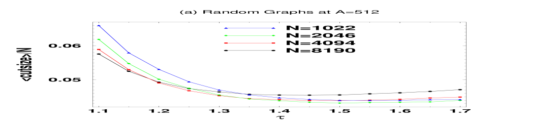
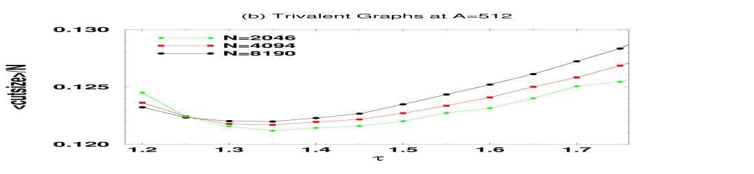
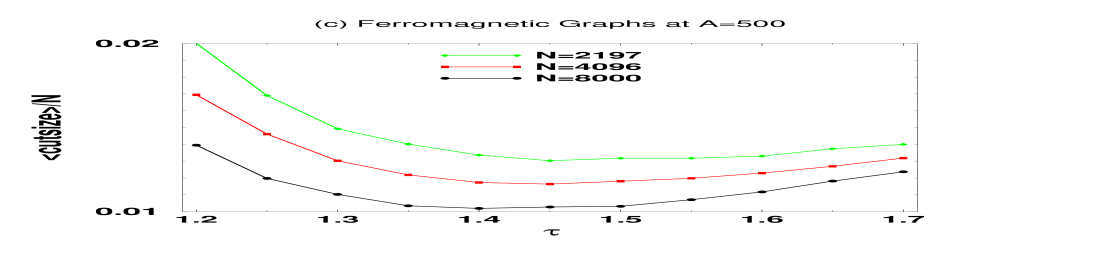
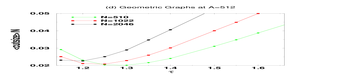
Figure 2: Cutsize found by EO (in units of $N$) as a function of $\tau$ at a fixed value of $A=t/N\approx 500$, averaged over all runs on all graphs of a given size $N$. Results are shown for (a) random graphs, (b) trivalent graphs, (c) ferromagnetic graphs, and (d) geometric graphs. For each type of graph the minimum shifts very slowly to smaller values of $\tau$ for increasing $N$.

While the optimal values for $\tau$ are similar for all types of graphs, there is a definite drift towards smaller values of $\tau$ for increasing $N$. Studies on spin glasses EO_PRL have led to similar observations, supporting the argument for the scaling of $\tau$ that we have given in Sec. III.3.2. Our data here do not cover a large enough range in $N$ to analyze in detail the dependence of $\tau$ on $\log N$. However, we can at least demonstrate that the results for trivalent graphs, where statistical errors are relatively small, are consistent with Eq. (6) above. For fixed $N$ but increasing values of $A=t/N$, we see in Fig. 3a that the optimal value of $\tau$ appears to increase linearly as a function of $\log A$ in the regime $1\ll A\ll N$. At the same time, fixing $A$ and increasing $N$, we see in Fig. 3b that the optimal value of $\tau$ appears to decrease linearly as a function of $1/\log N$, towards a value near $\tau=1$. Thus, for $1\ll A\ll N$, $\tau$ seems to be converging very slowly towards 1, with a finite $N$ correction of $\sim\log A/\log N$. This is in accordance with our estimate, Eq. (6), discussed earlier in Sec. III.3.2. (Note that at $A\approx 500$ in Figs. 2a-b, the optimal values for random and trivalent graphs are close to $\tau\approx 1.3$, consistent with Eq. (6). In contrast, in our long-time studies below, $A\gtrsim N$ and a value of $\tau=1.45$ seems preferable, consistent with Fig. 3a.)

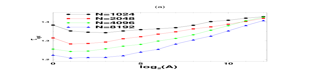
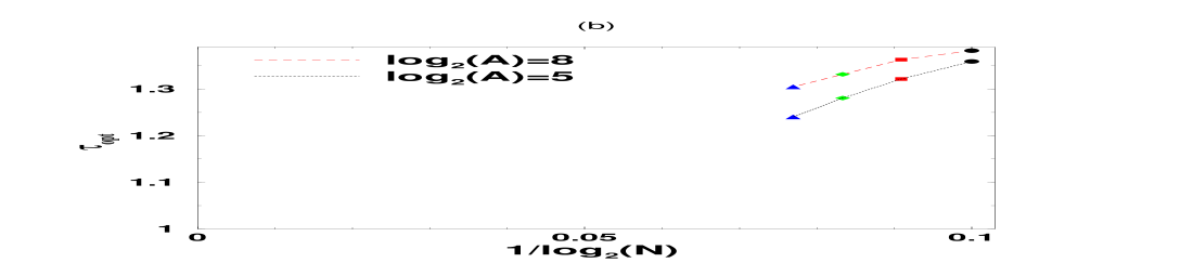
Figure 3: Plot of $\tau_{\rm opt}$ for trivalent graphs as a function of (a) $\log_{2}(A)=\log_{2}(t/N)$ for various fixed values of $N$ and (b) $1/\log_{2}(N)$ for various fixed values of $A=t/N$. These data points were determined by performing runs as in Fig. 2b, and finding the minimum of a quartic fit to data obtained at $\tau=1.2,~{}1.25,~{}1.3,\ldots,~{}1.95$. In (a) the data increase roughly linearly with $\log_{2}(A)$ in the regime $1\ll A\ll N$ at fixed $N$, while in (b) the data extrapolate roughly toward $\tau=1$ for $N\to\infty$ at fixed $A$, both in accordance with Eq. 6. For $A\lesssim 1$ this scaling appears to break down, while for $A\gtrsim N$ the linear scaling happens to remain valid. Note that the values of $\tau_{\rm opt}$ in (b) correspond to the data points in (a) for $\log_{2}(A)=5$ and 8.

The foregoing data, including the results plotted in Figs. 2a-d, arise from averages ${\overline{\langle m(t)\rangle}}$ over all runs (denoted by $\langle\ldots\rangle$) and all instances (denoted by an overbar). But it is important to note that the conclusions drawn with respect to the optimal value of $\tau$ from these plots are valid only if there is little difference between the average run $\langle m(t)\rangle$ and the best run $m_{\rm best}$ for a particular instance. While this is the case for the random and trivalent graphs, there is a significant difference between $\langle m(t)\rangle$ and $m_{\rm best}$ for instances of ferromagnetic and geometric graphs, as is discussed later in Sec. IV.3.3. In fact, for geometric graphs (Fig. 6 below), average and best cutsizes often differ by a factor of 2 or 3! Fig. 2d indicates that the optimal value of $\tau$ for the average performance on geometric graphs of size $N=2046$ is below $\tau=1.2$. If we instead plot the fraction of runs that have come, say, within 20% of the best value $m_{\rm best}$ found by EO (which most likely is still not optimal) for each instance, the optimal choice for $\tau$ shifts to larger values, $\tau\approx 1.3$ (see Fig. 4).

We may interpret this discrepancy as follows. At lower values of $\tau$, EO is more likely to explore the basin of many local minima but also has a smaller chance of descending to the “bottom” of any basin. At larger values of $\tau$, all but a few runs get stuck in the basin of a poor local minimum (biasing the average) but the lucky ones have a greater chance of finding the better states. For geometric graphs, the basins seem particularly hard to escape from, except at the very low values of $\tau$ where EO is unlikely to move toward the basin’s minimum. Thus, in such cases we find that we get better average performance $\langle m(t)\rangle$ at a lower value of $\tau$, but the best result $m_{\rm best}$ of multiple runs is obtained at a higher value of $\tau$.

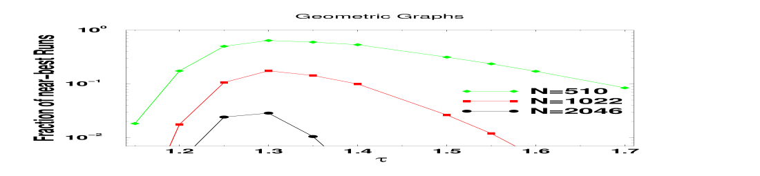
Figure 4: Fraction of EO runs on geometric graphs that have come within 20% of the best ever found (for each instance) as a function of $\tau$, for each value of $N$. Maxima indicate optimal choice of $\tau$ for finding a few good results among many runs. These maxima occur at higher values of $\tau$ than the minima corresponding to best average performance in Fig. 2. As seen below in Fig. 6, it becomes increasingly hard to come close to these best values.

Clearly, in order to obtain optimal performance of EO within a given runtime and for a given class of graphs, further study of the best choice of $\tau$ would be justified. But for an analysis of the scaling properties of EO with runtime and $N$, the specific details of how the optimal $\tau$ varies are not significant. Therefore, to simply the following scaling discussion, we will simply fix $\tau$ to a near-optimal value on each type of graph.

IV.3 Scaling behavior

IV.3.1 General results

As explained in Sec. III, the cutsize of the current configuration will fluctuate wildly at all times during an EO run and will not in itself converge. Instead, we have to keep track of the best configuration obtained so far during a run. Thus, even for times $t<t_{\rm max}$ during an EO run, we refer to the cutsize $m(t)$ of the current best configuration as the “result” of that run at time $t$. Examples of the stepwise manner in which $m(t)$ converges towards the optimal cutsize, for a particular instance of each type of graph, are given in Fig. 5. Up until times $t\sim N$, $m(t)$ drops rapidly because each update rectifies poor arrangements created by the random initial conditions. For times $t\gg N$, it takes collective rearrangements involving many vertices to (slowly) obtain further improvements.

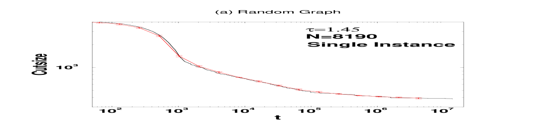
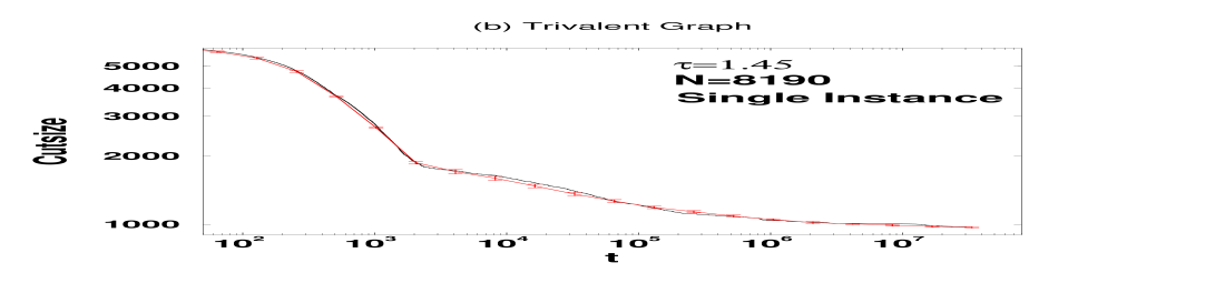
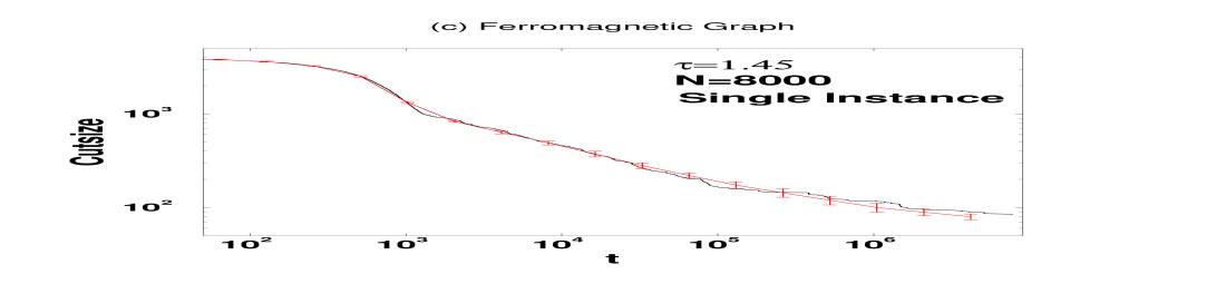
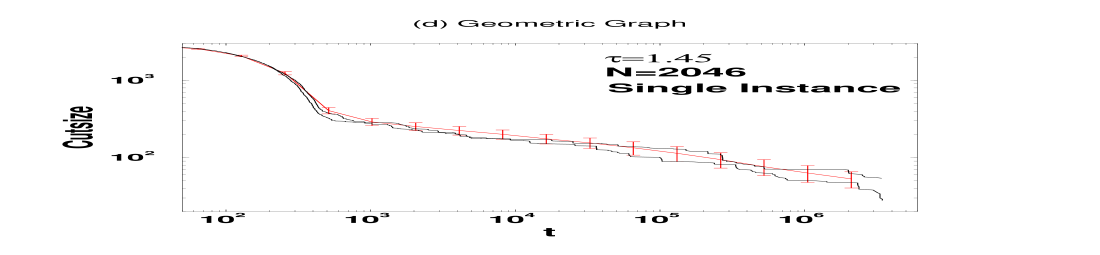
Figure 5: Log-log plot of the cutsize as a function of the number of update steps $t$ for a single (large) instance of a (a) random, (b) trivalent, (c) ferromagnetic and (d) geometric graph. The solid black line represents $m(t)$ for a single run, and the solid red line with error bars represents the average $\langle m(t)\rangle$ over all runs on that instance. In (a) and (b), error bars are very small, indicating that there are only small run-to-run fluctuations about $\langle m(t)\rangle$. By contrast, in (c) and (d), these run-to-run fluctuations are huge. In fact, for the geometric graph in (d) we have plotted two separate solid black lines representing two selected runs, one poor and one good one. This shows the large variations between runs that lead to the large error bars.

While during each run $m(t)$ decreases discontinuously, for the random and trivalent graphs the jumps deviate relatively little from that of the mean behavior obtained by averaging over many runs ($\langle\ldots\rangle$). Fluctuations, shown by the error bars in Figs. 5a-b, thus are small and will be neglected henceforth. For the ferromagnetic and geometric graphs, these fluctuations can be enormous. In Fig. 6 we compare the average performance ${\overline{\langle m\rangle}}$ with the best performance ${\overline{m_{\rm best}}}$ for each type of graph, at the maximal runtime $t_{\rm max}$ and averaged over all instances at each $N$. The results demonstrate that for random and trivalent graphs the average and best results are very close, whereas for ferromagnetic and geometric graphs they are far apart (with even the scaling becoming increasingly different for the geometric case). Therefore, in the following we will consider scaling of the average results for the first two classes of graphs, but properties of the best results for the latter two.

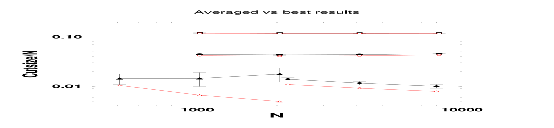
Figure 6: Log-log plot of the cutsize ${\overline{\langle m\rangle}}$, averaged over all runs and instances (filled symbol), and the best cutsize ${\overline{m}}_{\rm best}$ from all runs on an instance, averaged over all instances (open symbol). This is shown for random ($\circ$), trivalent ($\Box$), ferromagnetic ($\diamond$), and geometric graphs ($\triangle$), as a function of size $N$. The error bars refer only to run-to-run (and not instance-to-instance) fluctuations. For random and trivalent graphs, both average and best cutsizes scale linearly in $N$, as expected. For ferromagnetic and geometric graphs, the best results are several standard deviations better than the average results, with a widening gap for increasing $N$ on the geometric graphs. The scaling of $m_{\rm best}\sim N^{1/\nu}$ gives $\nu=1.3$ for ferromagnetic graphs, and is consistent with $\nu=2$ for geometric graphs.

IV.3.2 Random and trivalent graphs

Averaging $m(t)$ for any $t$ over all runs ($\langle\ldots\rangle$) and over all instances (overbar), we obtain the averaged cutsize

$${\overline{\langle m\rangle}}=m(N,t,\tau)$$ (8)

as a function of size $N$, runtime $t$, and parameter $\tau$. In Fig. 7 we plot $m(N,t,\tau)$ for random and trivalent graphs as a function of $t$, for each $N$ and at a fixed value $\tau=1.45$ that is near the optimal value for the maximal runtimes $t_{\rm max}$ (see Sec. IV.2). The error bars shown here are due only to instance-to-instance fluctuations, and are consistent with a normal distribution around the mean. (Note that the error bars are distorted due to the logarithmic abscissa.) The fact that the relative errors decreases with $N$ demonstrate that self-averaging holds and that we need only focus on the mean to obtain information about the typical scaling behavior of an EO run.

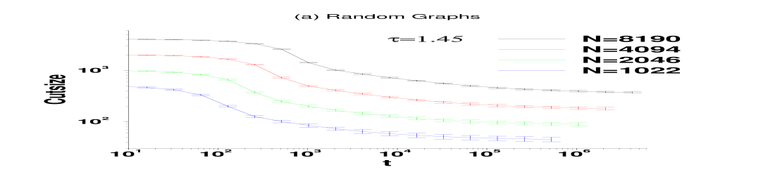
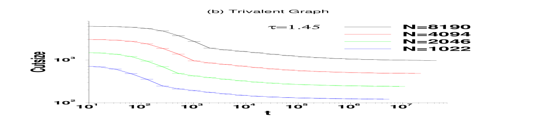
Figure 7: Log-log plot of the average cutsize $m(N,t,\tau)$ as a function of runtime $t$ at fixed $\tau=1.45$, for (a) random graphs and (b) trivalent graphs. The average is taken over runs as well as over instances (32 instances for random and 8 instances for trivalent graphs). Error bars represent instance-to-instance fluctuations only, and increase with $N$ much more slowly than the mean result. In each case, $N$ increases from bottom to top.

We wish to study the scaling properties of the function $m$ in Eq. (8). First of all, we find that generally

$$m(N,t,\tau)\sim N^{1/\nu}{\tilde{m}}(t/N,\tau)\quad(t\gg N\gg 1),$$ (9)

reflecting the fact that for EO, as well as for most other graph partitioning heuristics that are based on local search, runtimes scale linearly with $N$. (This is justified by the fact that each of the $N$ variables only has 2 states to explore. In, say, the traveling salesperson problem, by contrast, each of $N$ cities can be reconnected to $O(N)$ other cities, and so runtimes typically scale at least with $N^{2}$ JohnsonTSP .) In Fig. 8 we plot $m(N,t,\tau)/N$ for fixed $\tau=1.45$ as a function $t/N$. We find indeed that the data points from Fig. 7 collapse onto a single scaling curve ${\tilde{m}}(t/N,\tau)$, justifying the scaling ansatz in Eq. (9) for $\nu=1$. The scaling collapse is a strong indication that EO converges in $O(N)$ updates towards the optimal result, and also that the optimal cutsize itself scales linearly in $N$.

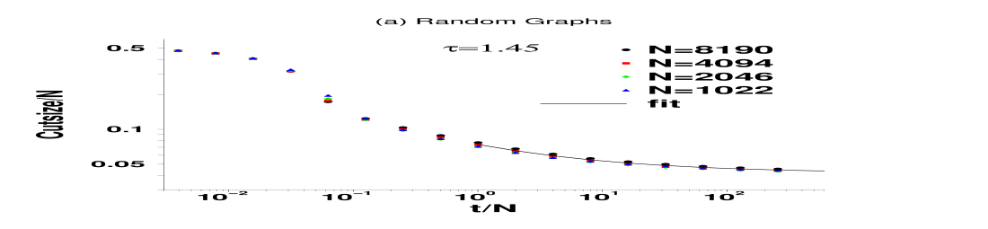
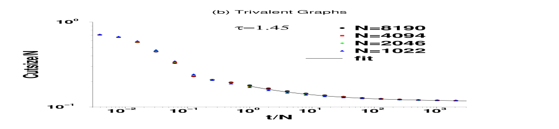
Figure 8: Scaling collapse of the data from Fig. 7 onto a single scaling curve ${\tilde{m}}(t/N,\tau)=m/N$ as a function of $t/N$ at fixed $\tau=1.45$, for (a) random graphs and (b) trivalent graphs. For $t>N$, data points are fitted to the power-law expression in Eq. (10) with numerical values given in Tab. 1.

Table 1: Sequence of values of the fit of Eq. (10) to the data in Fig. 8 for $t/N>1$, for each $N$.

Graph Type	Size $N$	$\langle{\tilde{m}}_{\rm opt}\rangle$	$C$	$\gamma$
Random	1022	0.0423	0.028	0.48
	2046	0.0411	0.029	0.46
	4094	0.0414	0.032	0.45
	8190	0.0425	0.034	0.44
Trivalent	1022	0.1177	0.052	0.43
	2046	0.1159	0.057	0.41
	4094	0.1159	0.062	0.41
	8190	0.1158	0.066	0.40

The scaling function ${\tilde{m}}$ appears to converge at large times to the average optimal result $\langle{\tilde{m}}_{\rm opt}\rangle=\langle m_{\rm opt}\rangle/N$ according to a power law:

$${\tilde{m}}(t/N,\tau)\sim\langle{\tilde{m}}_{\rm opt}\rangle+C\left({t\over N}\right)^{-\gamma}\quad(t\gg N\gg 1).$$ (10)

Fitting the data in Fig. 8 to Eq. (10) for $t/N>1$, we obtain for each type of graph a sequence of values for $\langle{\tilde{m}}_{\rm opt}\rangle$ and $\gamma$ for increasing $N$, given in Tab. 1. In both cases we find values for $\langle{\tilde{m}}_{\rm opt}\rangle/N$ that are quite stable, while the values for $\gamma$ slowly decrease with $N$. The variation in $\gamma$ as a function of $N$ may be related to the fact that for a fixed $\tau$, EO’s performance at fixed $A=t/N$ deteriorates logarithmically with $N$, as seen in Sec. IV.2. Even with this variation, however, the values of $\gamma$ for both types of graph are remarkably similar: $\gamma\approx 0.4$. This implies that in general, on graphs without geometric structure, we can halve the approximation error of EO by increasing runtime by a factor of 5–6. This power-law convergence of EO is a marked improvement over the mere logarithmic convergence conjectured for simulated annealing Science on NP-hard problems Grest .

Finally, the asymptotic value of $\langle{\tilde{m}}_{\rm opt}\rangle$ obtained for the trivalent graphs can be compared with previous simulations Banavar ; EOperc . There, the “energy” ${\cal E}=-1+4\langle{\tilde{m}}_{\rm opt}\rangle/3$ was calculated using the best results obtained for a set of trivalent graphs. Ref. Banavar using simulated annealing obtained ${\cal E}=-0.840$, while in a previous study with EO EOperc we obtained ${\cal E}=-0.844(1)$. Our current, somewhat more careful extrapolation yields $\langle{\tilde{m}}_{\rm opt}\rangle=0.1158N$ or ${\cal E}=-0.845(1)$. Even though this extrapolation is based on the average data rather than only the best of all runs, the very low fluctuations between runs (see Figs. 5b and 6) indicate that the result for ${\cal E}$ would not change significantly. Thus, the replica symmetric solution proposed in Refs. M+P ; W+S for this version of the GBP, which gives a value of ${\cal E}=-2\times 0.7378/\sqrt{3}=0.852$, seems to be excluded.

IV.3.3 Ferromagnetic and geometric graphs

Unlike on the preceding graphs, EO gives significantly different results for an average run and for the best run on geometrically structured graphs (see Figs. 5 and 6). In Fig. 6, at least the results from the best run (averaged over all instances) comes close to the scaling behavior expected from the considerations in Sec. II.3: a fit gives $\nu\approx 1.3$ for ferromagnetic, and $\nu\approx 2$ for geometric graphs, while the theory predicts $\nu=3/2$ and $\nu=2$ respectively. But even these best cutsizes themselves vary significantly from one instance to another. Thus, it is certainly not useful to study the “average” run. Instead, we will consider the result of each run at the maximal runtime $t_{\rm max}$, extract the best out of $k$ runs, and study these results as a function of increasing $k$.

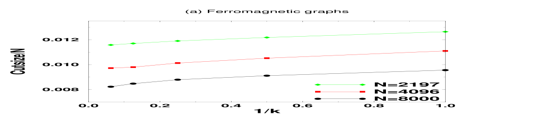
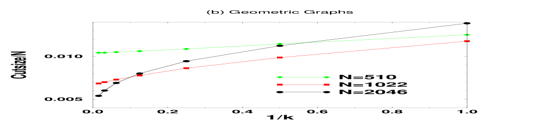
Figure 9: Extrapolation plot for the best-of-$k$ trials for (a) ferromagnetic graphs at $\tau=1.4$ and (b) for geometric graphs at $\tau=1.3$. The data for this plot are extracted from the results at $t_{\rm max}$, averaging the best-of-$k$ results over 16 instances for ferromagnetic, and 64 instances for geometric graphs. For comparison, the leftmost data point for each $N$ at $k=16$ for ferromagnetic graphs and at $k=64$ for geometric graphs corresponds to the “best” results plotted in Fig. 6 for those graphs.

Fig. 9 shows the difficulty of finding good runs with near-optimal results for increasing size $N$. While for ferromagnetic graphs it is possible that acceptable results may be obtained without increasing $k$ dramatically, for geometric graphs an ever larger number of runs seems to be needed at large $N$. It does not appear possible to obtain consistent good near-optimal results at a fixed $k$ for increasing $N$.

We saw in Sec. IV.3.2 that for random graphs, computational time is well spent on a few, long EO runs per instance. We can not address in detail the question of whether, for geometrically defined graphs, computational time is better spent on $k$ independent EO-runs with $t_{\rm max}$ update steps or, say, on a single EO-run with $k\times t_{\rm max}$ update steps. While experience with our data would indicate the former to be favorable, an answer to this question depends significantly on $N$ and, of course, on the choice of $\tau$ (see Sec. IV.2). Here we consider this question merely for a single value, $\tau=1.3$, for which we have run EO on the same 64 geometric graphs up to 16 times longer than $t_{\rm max}$, but using only $k=4$ restarts. In each of these 4 runs on an instance we recorded the best result seen at multiples $n\times t_{\rm max}$ with $n=1,2,4,8$, and 16. For example, the best-of-4 runs at $n=1$ of this runtime corresponds to the best-of-$k$ results in Fig. 9 for $k=4$, while $n=16$ would correspond to the same amount of running time as $k=64$. Fig. 10 shows that fewer but longer runs are slightly more successful for larger $N$.

Finally, we have also used the clustering algorithm described in Sec. III.3.4 and Ref. BoPe1 on this set of 64 graphs with $\tau=1.3$. For comparison, we again use the best-of-4 runs with averages taken at times $n\times t_{\rm max}$, $n=1,2,$ and 4. Results at short runtimes improve by a huge amount with such a procedure, but its advantage is eventually lost at longer runtimes. While this procedure is cheap, easy, and apparently always successful for geometric graphs, our experiments indicate that its effect may be less significant for random graphs and may actually result in diminished performance when used for trivalent graphs in place of random initial conditions. Clearly, clustering is tailored more toward geometric graphs satisfying a triangular inequality.

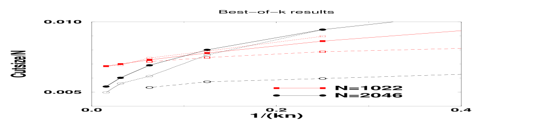
Figure 10: Equivalent-runtime comparison between different strategies to improve EO results on geometric graphs for $N=1022$ and 2046 at $\tau=1.3$. The horizontal axis is proportional to the inverse of the number of updates used, $t=k\times n\times t_{\rm max}$. Filled symbols refer to the $n=1$ results for geometric graphs already plotted in Fig. 9b, where $k$ is varied. Open symbols on the dotted lines refer to the $k=4$ (best-of-4) results, where $n$ is varied. Opaque symbols on the dashed line refer to $k=4$ results as well, but using initial conditions generated by a clustering algorithm (see Sec. III.3.4). At sufficiently long runtime all strategies are about equal, though with fewer but longer runs having a slight edge over more and shorter runs for large $N$. Even the advantages of a non-random initial configuration become less significant at longer runtimes.

V Conclusions

Using the classic combinatorial optimization problem of bipartitioning graphs as an application, we have demonstrated a variety of properties of the extremal optimization algorithm. We have shown that for random graphs, EO efficiently approximates the optimal solution even at large size $N$, with an average approximation error decreasing over runtime $t$ as $t^{-0.4}$. For sparse, geometrically defined graphs, finding the ideal (sub-dimensional) interface partitioning the graph becomes ever more difficult as size $N$ increases. EO, like other local search methods JohnsonGBP , gets stuck ever more often in poor local minima. However, when we consider the best out of multiple runs with the EO algorithm, we recover results close to those predicted by theoretical arguments.

We believe that many of our findings here, notably with regard to EO’s fitness definition and the update procedure using the parameter $\tau$, are generic for the algorithm. Our results for optimizing 3-coloring and spin glasses appear to bear out such generalizations EO_PRL . In view of this observation, a firmer theoretical understanding of our numerical findings would be greatly desirable. The nature of EO’s performance derives from its large fluctuations; the price we pay for this is the loss of detailed balance, which is the theoretical basis for other physically-inspired heuristics, such as simulated annealing Science . On the other hand, unlike in simulated annealing, we have the advantage of dealing with a Markov chain that is independent of time Aarts . This suggests that our method may indeed be amenable to theoretical analysis. We believe that the results EO delivers, as a simple and novel approach to optimization, justify the need for further analysis.

VI Acknowledgements

We would like to thank the participants of the Telluride Summer workshop on complex landscapes, in particular Paolo Sibani, for fruitful discussions, and Jesper Dall for confirming many of our results in his master thesis at Odense University. This work was supported by the University Research Committee at Emory University, and by an LDRD grant from Los Alamos National Laboratory.

References

- (1) M. Mezard, G. Parisi, and M. A. Virasoro, Spin Glass Theory and Beyond (World Scientific, Singapore, 1987).
- (2) G. S. Grest, C. M. Soukoulis, and K. Levin, Phys. Rev. Lett. 56, 1148 (1986).
- (3) J. Dall and P. Sibani, “Faster Monte Carlo Simulations at Low Temperatures: The Waiting Time Method,” unpublished.
- (4) T. Klotz and S. Kobe, J. Phys. A 27, L95 (1994); K. F. Pal, Physica A 223, 283 (1996); A. K. Hartmann, Phys. Rev. E 60, 5135 (1999); M. Palassini and A. P. Young, Phys. Rev. Lett. 85, 3017 (2000); A. Möbius, A. Neklioudov, A. Díaz-Sánchez, K. H. Hoffmann, A. Fachat, and M. Schreiber, Phys. Rev. Lett. 79, 4297 (1997).
- (5) H. Frauenkron, U. Bastolla, E. Gerstner, P. Grassberger, and W. Nadler, Phys. Rev. Lett. 80, 3149 (1998); E. Tuzel and A. Erzan, Phys. Rev. E 61, R1040 (2000).
- (6) G. Toulouse, Comm. Phys. 2, 115 (1977).
- (7) See Landscape Paradigms in Physics and Biology, edited by H. Frauenfelder, et al. (Elsevier, Amsterdam, 1997).
- (8) S. Boettcher and A. G. Percus, Artificial Intelligence 119, 275 (2000).
- (9) S. Boettcher and A. G. Percus, in GECCO-99: Proceedings of the Genetic and Evolutionary Computation Conference (Morgan Kaufmann, San Francisco, 1999), p. 825.
- (10) P. Bak, C. Tang, and K. Wiesenfeld, Phys. Rev. Lett. 59, 381 (1987).
- (11) S. Boettcher, A. G. Percus, and M. Grigni, Lecture Notes in Computer Science 1917, 447 (2000); S. Boettcher, Computing in Science and Engineering 2:6, 75 (2000).
- (12) J. Holland, Adaptation in Natural and Artificial Systems (University of Michigan Press, Ann Arbor, 1975).
- (13) S. Kirkpatrick, C. D. Gelatt, and M. P. Vecchi, Science 220, 671 (1983).
- (14) S. Boettcher, J. Phys. A 32, 5201 (1999).
- (15) P. Cheeseman, B. Kanefsky, and W. M. Taylor, in Proceedings of IJCAI-91, edited by J. Mylopoulos and R. Rediter (Morgan Kaufmann, San Mateo, CA, 1991), p. 331.
- (16) S. Boettcher, A. G. Percus, G. Istrate, and M. Grigni (in preparation).
- (17) S. Boettcher and A. G. Percus, Phys. Rev. Lett. (in press), cond-mat/0010337.
- (18) J. Dall, Master’s Thesis, Odense University Physics Department, Nov. 2000.
- (19) M. R. Garey and D. S. Johnson, Computers and Intractability, A Guide to the Theory of NP-Completeness (W. H. Freeman, New York, 1979); G. Ausiello, P. Crescenzi, G. Gambosi, V. Kann, A. Marchetti-Spaccamela, and M. Protasi, Complexity and Approximation (Springer, Berlin, 1999).
- (20) C. J. Alpert and A. B. Kahng, Integration: The VLSI Journal 19, 1 (1995).
- (21) B. A. Hendrickson and R. Leland, in Proceedings of Supercomputing ’95, San Diego, CA (1995).
- (22) P. Erdös and A. Rényi, in The Art of Counting, edited by J. Spencer (MIT, Cambridge, 1973); B. Bollobas, Random Graphs (Academic Press, London, 1985).
- (23) K. Y. M. Wong and D. Sherrington, J. Phys. A 20, L793 (1987); K. Y. M. Wong, D. Sherrington, P. Mottishaw, R. Dewar, and C. De Dominicis, J. Phys. A 21, L99 (1988).
- (24) J. R. Banavar, D. Sherrington, and N. Sourlas, J. Phys. A 20, L1 (1987).
- (25) M. Mezard and G. Parisi, Europhys. Lett. 3, 1067 (1987).
- (26) D. S. Johnson, C. R. Aragon, L. A. McGeoch, and C. Schevon, Operations Research 37, 865 (1989).
- (27) I. Balberg, Phys. Rev. B 31, R4053 (1985).
- (28) Y. T. Fu and P. W. Anderson, J. Phys. A 19, 1605 (1986).
- (29) S. Kirkpatrick and B. Selman, Science 264, 1297 (1994); R. Monasson, R. Zecchina, S. Kirkpatrick, B. Selman, and L. Troyansky, Nature 400, 133 (1999); also Random Struct. Alg. 15, 414 (1999); See Frontiers in problem solving: Phase transitions and complexity, Special issue of Artificial Intelligence 81:1–2 (1996).
- (30) G. Karypis and V. Kumar, METIS, a Software Package for Partitioning Unstructured Graphs, see http://www-users.cs.umn.edu/~karypis/metis (METIS is copyrighted by the Regents of the University of Minnisota).
- (31) S. Boettcher, unpublished.
- (32) P. Bak and K. Sneppen, Phys. Rev. Lett. 71, 4083 (1993).
- (33) S. J. Gould and N. Eldridge, Paleobiology 3, 115 (1977).
- (34) D. R. Chialvo and P. Bak, Neuroscience 90, 1137 (1999).
- (35) Modern Heuristic Techniques for Combinatorial Problems, edited by C. R. Reeves (Wiley, New York, 1993).
- (36) M. Paczuski, S. Maslov, and P. Bak, Phys. Rev. E 53, 414 (1996).
- (37) D. S. Johnson, Lecture Notes in Computer Science 443, 446 (1990).
- (38) Local Search in Combinatorial Optimization, edited by E. H. L. Aarts and J. K. Lenstra (Wiley, New York, 1997).