Connecting the vulcanization transition to percolation

Abstract

The vulcanization transition is addressed via a minimal replica-field-theoretic model. The appropriate long-wave-length behavior of the two- and three-point vertex functions is considered diagrammatically, to all orders in perturbation theory, and identified with the corresponding quantities in the Houghton-Reeve-Wallace field-theoretic approach to the percolation critical phenomenon. Hence, it is shown that percolation theory correctly captures the critical phenomenology of the vulcanization transition associated with the liquid and critical states.

I Introduction and overview

The vulcanization transition (henceforth denoted VT) is the generic equilibrium phase transition from a parent liquid state of matter to an amorphous solid state, driven by the imposition of a sufficient density of permanent random constraints between the constituents of the liquid. In the most common setting of the VT, the constituents of the liquid are macromolecules, the locations of which provide the annealed random (i.e. thermally equilibrating) variables. The constraints are commonly provided by covalent chemical bonds (i.e. cross-links), and impart quenched randomness upon the system. Over the past few years, a rather detailed description of the VT has been developed, ranging from a mean-field theory of the emergent amorphous solid state (including its structural [1, 2] and elastic properties [3], and its stability [4]; for reviews, see Refs. [5, 6]) to the critical properties of the VT itself [7].

The present Paper aims to extend the description of the critical properties of the VT by exploring its relationship with the percolation transition (henceforth denoted PT; for a review, see Ref. [8]). This relationship, which has long been anticipated on physical grounds [9, 10], has recently found support both at the mean-field level [1, 5], and beyond, via a renormalization-group approach [7]. Specifically, it was recently shown that the order-parameter correlator near the VT (which probes for relative localization of particles) and its physical analog in PT (viz., the connectedness function) are governed by the same critical exponents, at least to first order in an expansion about the upper critical dimension six [7].

The central result of the present Paper is the explicit reduction of certain basic critical properties of the VT to equivalent basic critical properties of the PT [11]. As we shall see, this reduction can be accomplished via an exact diagrammatic analysis of the complete perturbative expansion of the appropriate vertex functions of the VT. These are shown to furnish, in the replica limit, precisely the field-theoretic formulation of the PT due to Houghton, Reeve and Wallace [12] (which henceforth we shall refer to as HRW). Hence, we establish that the critical properties of the VT and the PT are identical, not just to first order but to all orders in the departure of the spatial dimension $d$ from the upper critical dimension.

It is worth observing that the VT and the PT do, nevertheless, represent distinct physical phenomena. This is exemplified, e.g., by the amorphous solid state that emerges at the VT, which does not have an evident counterpart in PT. Another point of distinction is revealed by the role of fluctuations in low-dimensional systems, which are expected to have qualitatively different impacts on the states emerging at the VT and the PT [13]. Yet another point of distinction concerns the nature of the degrees of freedom involved in the description of the VT and the PT. The former arises in systems having both quenched and equilibrating randomness, whereas the latter takes place in systems involving just one type of randomness (typically taken to be the quenched randomness); see Ref. [13].

After completion of the present work we learned of the elegant work of Janssen and Stenull [14], conducted independently of and simultaneously with the present work, which builds on earlier work on random resistor networks and percolation to arrive at, inter alia, essentially the same results as those contained in the present paper via a related approach.

II Minimal model of the vulcanization transition

Our analysis is based upon a minimal model of the VT that accounts for thermal fluctuations in the positions of the constituents of the parent liquid, short-range repulsions between these constituents, and permanent random constraints (e.g. resulting from cross-linking) which explicitly reduce the collection of configurations accessible to the constituents. This minimal model yields a rich mean-field picture of the structure and elastic response of the amorphous solid state, the former aspect having been verified by the computer simulations of Barsky and Plischke [15].

The minimal model for the VT can be built (in the spirit of the Landau-Wilson scheme for continuous phase transitions) on the general basis of symmetry considerations and a gradient expansion [2]. The appropriate order parameter $\Omega$, whose expectation value detects the emergence of the amorphous solid state, has been discussed elsewhere [16]. The quenched random constraints are accounted for via the replica technique, which incorporates the Deam-Edwards model [17] for their statistics (viz. the statistics of the random constraints are determined by the instantaneous correlations of the unconstrained system). The additional replica associated with the Deam-Edwards model leads to a situation in which one considers the $n\to 0$ limit of a system of not of $n$ but of $n+1$ replicas.

The resulting Landau-Wilson effective Hamiltonian takes the form of a cubic field theory involving the field $\Omega$, the argument of this field lying in $(n+1)$-fold replicated $d$-dimensional space:

$${\cal S}\big{(}\Omega\big{)}=\frac{1}{V^{n+1}}\frac{1}{2}\sum_{\hat{k}\in{{\rm HRS}}}\Big{(}r_{0}+\hat{k}\cdot\hat{k}\Big{)}\big{|}\Omega(\hat{k})\big{|}^{2}+\,\,\,\frac{1}{V^{2(n+1)}}\frac{g}{3!}\!\!\!\!\sum_{\,\,\,\,\hat{k}_{1},\hat{k}_{2},\hat{k}_{3}\in{\rm HRS}}\!\!\!\!\Omega({\hat{k}}_{1})\,\Omega({\hat{k}}_{2})\,\Omega({\hat{k}}_{3})\,\delta_{{\hat{k}_{1}}+{\hat{k}_{2}}+{\hat{k}_{3}},{\hat{0}}}\,.$$ (1)

The free-energy density $f$ is (up to uninteresting factors that we shall ignore) related to this Hamiltonian via $f\propto\lim_{n\to 0}n^{-1}{\ln\{\int{\cal D}\Omega\exp(-{\cal S})\}}$; the functional integral is taken over the independent components of $\Omega$ that feature in ${\cal S}$. In ${\cal S}$, the quantity $r_{0}$ is the VT control parameter which, near the VT, is linearly related to the density of random constraints. (To ease comparison with the HRW field theory of the PT, the coefficients and fields featuring in ${\cal S}$ are not defined exactly as they have been in our earlier works [18].)  The symbol ${\hat{k}}$ denotes the replicated wave vector $\{{\bf k}^{0},{\bf k}^{1},\ldots,{\bf k}^{n}\}$; the extended scalar product $\hat{k}\cdot\hat{c}$ is denoted ${\bf k}^{0}\cdot{\bf c}^{0}+{\bf k}^{1}\cdot{\bf c}^{1}+\cdots+{\bf k}^{n}\cdot{\bf c}^{n}$. The specification HRS arises from the following considerations. Consider the space of replicated wave vectors $\hat{k}$. We decompose this space into three disjoint sets: (i) the higher replica sector HRS, which consists of those $\hat{k}$ containing at least two nonzero component-vectors ${\bf k}^{\alpha}$; (ii) the one replica sector 1RS, which consists of those $\hat{k}$ containing exactly one nonzero component-vector ${\bf k}^{\alpha}$; and (iii) the zero replica sector 0RS, which consists of the vector ${\hat{k}}=\hat{0}$. This decomposition is illustrated schematically in Fig. 1 for the case of two replicas. It is especially straightforward to visualize this decomposition if the volume of the system is kept finite (and periodic boundary conditions are imposed) so that replicated plane waves with discrete, equally spaced, replicated wave vectors provide the natural complete set of functions.

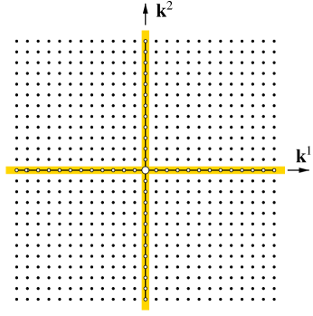
FIG. 1.: Decomposition of the space of replicated wave vectors. Off-axis wave vectors lie in the HRS; on-axis (but off-origin) wave vectors lie in the 1RS; the wave vector at the origin is the 0RS.

The symbol $\sum_{\hat{k}\in{{\rm HRS}}}$ indicates a summation over the replicated wave vector $\hat{k}$, subject to the restriction that $\hat{k}$ lies in HRS. This condition on the summation over $\hat{k}$ is essential. Physically, it reflects the fact that no macroscopically inhomogeneous modes (such as crystalline modes) order or fluctuate critically in the vicinity of the VT, such modes being stabilized by the excluded-volume interactions. Mathematically, this condition reduces the symmetry of the theory from one that contains the rotation group in replicated $(n+1)d$-dimensional space to one that contains only rotations within each individual replica, along with the permutation of the replicas.

III Demonstrating the equivalence of the critical properties of the vulcanization and percolation transitions

A Overall strategy

We now explain the strategy that we shall use to relate the VT and the PT. We shall focus on the replica limit of the long-wave-length behavior of the two- and three-point vertex functions, $\Gamma_{n}^{(2)}(\hat{k})$ and $\Gamma_{n}^{(3)}({\hat{k}}_{1},{\hat{k}}_{2})$ in the VT field theory. The physical significance $\Gamma_{n}^{(2)}(\hat{k})$ as a probe of connectedness has been elucidated in Ref. [7]. Now, the symmetry of the VT field theory dictates that the only suitably invariant term quadratic in the wave vector $\hat{k}$ is $\hat{k}\cdot\hat{k}$. Thus, in a long-wave-length expansion for $\Gamma_{n}^{(2)}(\hat{k})$, we have

$$\Gamma_{n}^{(2)}({\hat{k}}) = \Gamma_{n}^{(2)}({\hat{0}})+{1\over{(n+1)d}}\sum_{\alpha=0}^{n}\left({\partial\over{\partial{\bf k}^{\alpha}}}\cdot{\partial\over{\partial{\bf k}^{\alpha}}}\right)\Gamma_{n}^{(2)}(\hat{k})\Big{|}_{{\hat{k}}={\hat{0}}}\,\,{\hat{k}}\cdot{\hat{k}}+\cdots$$ (3)

$$= A_{n}+B_{n}{\hat{k}}\cdot{\hat{k}}+\cdots\,\,.$$ (4)

As the upper critical dimension for the VT is six, and this is the dimension about which one may imagine expanding, general renormalizability considerations demand that just these two vertex functions ($\Gamma_{n}^{(2)}$ and $\Gamma_{n}^{(3)}$) contain the primitive divergences, and do so via the constants $A_{n}$, $B_{n}$ and $C_{n}\equiv\Gamma_{n}^{(3)}({\hat{0}},{\hat{0}})$ (see Ref. [19]).

Having identified the quantities central to a renormalization-group analysis of the VT, we shall establish that these quantities are identical, in the replica limit, to the corresponding quantities in percolation theory. To do this we shall make use of a convenient representation of the critical properties of percolation theory, viz., the HRW field theory representation [12]. So that we know what we need to make contact with, we pause to give a brief account of this HRW representation, the Landau-Wilson Hamiltonian for which is given by

$${\cal H}=\int d^{d}x\left\{\frac{1}{2}(\nabla\phi)^{2}-\frac{1}{2}(\nabla\psi)^{2}+\frac{1}{2}r_{0}(\phi^{2}-\psi^{2})+\frac{g}{3!}(\phi+\psi)^{3}\right\},$$ (5)

where $\phi$ is an ordinary field but $\psi$ is a ghost field. As HRW have shown, provided one enforces the rule that only graphs that are connected by $\phi$-lines are included, the two- and three-point $\phi$ vertex functions are identical (order by order in perturbation theory in the coupling constant $g$) to those of the one-state (i.e. percolation) limit of the Potts model. We mention, in passing, that this HRW representation consists of fields residing on $d$-dimensional space, and does not necessitate the taking of a replica (or Potts) limit. However, it does require the additional rule by which certain diagrams are excluded by hand.

Our strategy is as follows. Consider the standard Feynman diagram expansion for the two- and three-point vertex functions of the VT field theory in powers of the coupling constant $g$ in the Hamiltonian (1). (i) To deal with the constraint that the internal wave vectors in the resulting diagrams reside in the HRS, we relax this constraint on summations over internal wave vectors but compensate for this by making appropriate subtractions of terms. (ii) Next, we observe that all diagrams for the two- and three-point vertex functions can be organized into two categories: those in which there is at least one route between every pair of external points via propagators having unconstrained wave vectors (which we call freely-connected diagrams); and the remaining diagrams, in which there is at least one pair of external points between which no paths exist consisting solely of propagators having unconstrained wave vectors (which we call freely-unconnected diagrams). Having made this categorization, we show that the appropriate version of wave-vector conservation renders the freely-unconnected diagrams negligible in the thermodynamic limit, leaving us with a representation that is already reminiscent on the HRW approach. (iii) At this stage we have reduced the construction of the two- and three-point vertex functions to the computation of freely-connected diagrams only. Next, via a straightforward combinatorial analysis, we show that, in the replica limit, only a small class of diagrams survive. (iv) Finally, we explain how, again in the replica limit, the values of the remaining diagrams are precisely those occurring in the HRW prescription for percolation. We now set about implementing this strategy.

B Relaxing the constraint to higher replica sector wave vectors

In the VT field theory the internal wave vectors occurring in the Feynman diagrams are constrained to lie in the HRS. In order to perform summations over these wave vectors, it is convenient to work with the continuum of wave vectors (i.e. to take the thermodynamic limit) rather than the discrete lattice of them. In order to be able to take this limit, we re-express summations over HRS wave vectors in terms of unconstrained summations over $(n+1)d$-dimensional wave vectors, together with further unconstrained summations over $d$-dimensional wave vectors (and certain trivial additional terms). To do this, we note that for a generic function $F(\hat{k})$ we have

$$\sum_{\hat{k}\in{{\rm HRS}}}F(\hat{k}) = \sum_{\hat{k}}\left(1-\Big{(}\sum_{\alpha=0}^{n}\sum_{{\bf q}\neq{\bf 0}}\delta_{{\bf k}^{\alpha},{\bf q}}\prod_{\beta(\neq\alpha)}\delta_{{\bf k}^{\beta},{\bf 0}}\Big{)}-\delta_{\hat{k},\hat{0}}\right)F(\hat{k})$$ (7)

$$= \sum_{\hat{k}}\left(1-\Big{(}\sum_{\alpha=0}^{n}\sum_{{\bf q}}\delta_{{\bf k}^{\alpha},{\bf q}}\prod_{\beta(\neq\alpha)}\delta_{{\bf k}^{\beta},{\bf 0}}\Big{)}-n\delta_{\hat{k},\hat{0}}\right)F(\hat{k})$$ (8)

$$= \sum_{\hat{k}}F(\hat{k})-\sum_{\alpha=0}^{n}\sum_{{\bf q}^{\alpha}}F({\bf 0},\ldots,{\bf 0},{\bf q}^{\alpha},{\bf 0},\ldots)-nF(\hat{0}),$$ (9)

which effects the re-expression of the summations just described. Note that, as it always comes with the factor $n$, the $\delta_{\hat{k},\hat{0}}$ term will vanish in the replica limit, and can therefore be safely ignored. We shall refer to the wave vectors included in the term $\sum_{\alpha}\sum_{{\bf q}}$ as lower replica sector (LRS) wave vectors. Via these steps one can relax a constrained summation over HRS wave vectors, instead freely summing over all replicated wave vectors, provided one compensates by augmenting the summand with the factor

$$1-\sum_{\alpha=0}^{n}\sum_{{\bf q}}\delta_{{\bf k}^{\alpha},{\bf q}}\prod_{\beta(\neq\alpha)}\delta_{{\bf k}^{\beta},{\bf 0}}\,\,.$$ (10)

How does this constraint relaxation manifest itself in the setting of Feynman diagram computations? One simply augments every internal propagator $V^{n+1}G_{0}(\hat{k})$ with a factor (10):

$$G_{0}(\hat{k})\equiv\frac{1}{r_{0}+\hat{k}\cdot\hat{k}} \longrightarrow \frac{1-\sum_{\alpha}\sum_{{\bf q}}\delta_{{\bf k}^{\alpha},{\bf q}}\prod_{\beta(\neq\alpha)}\delta_{{\bf k}^{\beta},{\bf 0}}}{r_{0}+\hat{k}\cdot\hat{k}}$$ (12)

$$= \frac{1}{r_{0}+\hat{k}\cdot\hat{k}}-\frac{1}{r_{0}+\hat{k}\cdot\hat{k}}\sum_{\alpha=0}^{n}\sum_{{\bf q}}\delta_{{\bf k}^{\alpha},{\bf q}}\prod_{\beta(\neq\alpha)}\delta_{{\bf k}^{\beta},{\bf 0}}.$$ (13)

How this decomposition is expressed diagrammatically is shown in Fig. 2.

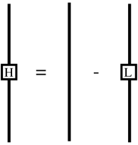
FIG. 2.: Decomposition of an HRS propagator (indicated by H) into an unconstrained propagator (the unadorned line), less an LRS propagator (indicated by L).

In this manner, each HRS internal line in a Feynman diagram can be decomposed into an unconstrained internal line, less an LRS internal line. Thus, the various vertex functions can be expressed in terms of Feynman diagrams composed of unconstrained lines together with as LRS internal lines. Note, for future reference, that physically meaningful vertex functions have external wave vectors in the HRS.

We illustrate this decomposition for the case of a simple diagram in Fig. 3. More generally, we arrive at the following modified Feynman rules for the VT field theory: (i) Write down all diagrams arising from the original theory. In these diagrams all wave vectors are constrained to the HRS. (ii) Replace each diagram with the collection of diagrams obtained by allowing each internal line to carry either an unconstrained replicated wave vector or a LRS wave vector. (Thus, a diagram with $L$ internal lines spawns a total of $2^{L}$ diagrams.)  Identically-valued diagrams can be represented by a single diagram, together with a suitable combinatorial factor (see, e.g., the factor of 2 in Fig 3). (iii) Provide a factor of $-1$ for each LRS internal line. At this stage we observe that the combinatorics of our diagrammatic expansion coincides with those of the HRW expansion, provided one identifies the internal unconstrained and LRS lines of the VT theory with, respectively, the corresponding internal $\phi$- and $\psi$-lines of the HRW representation.

FIG. 3.: Decomposition of the one-loop diagram for the two-point vertex function. On the right-hand side of this equation, the first and second diagrams are freely-connected diagrams, and the third is a freely-unconnected diagram.

We have, however, yet to show that the diagrams removed by hand in HRW can be safely omitted from the VT theory, and that the numerical values of the (replica limits of) the VT diagrams are identical to those of the HRW diagrams. We shall establish these facts in the following subsections.

C Elimination of freely-unconnected diagrams

We remind the reader that in the HRW theory for the two- and three-point $\phi$-field (i.e. the physical) vertex functions, one is instructed to remove, by hand, those diagrams in which there is at least one pair of external points between which no paths exist consisting solely of $\phi$-field propagators. The corresponding diagrams in the VT theory are those in which there is at least one pair of external points between which no paths exist consisting solely of propagators having unconstrained wave vectors, i.e., freely-unconnected diagrams. We now show that these freely-unconnected diagrams of the VT theory automatically vanish in the thermodynamic limit.

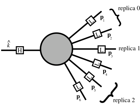
FIG. 4.: Schematic illustration of a piece of a diagram in the VT field theory obtained by cutting LRS lines in a freely-unconnected diagram. Note that the wave vector $\hat{k}$ flowing through the external point lies in the HRS. The shaded circle represents any way to connect the exhibited lines using the cubic interaction vertex, unconstrained propagators and LRS propagators.

To do this, consider a generic VT theory diagram for the two- or three-point vertex functions. Observe that freely-unconnected diagrams have the following property: as there exists a pair of external points not connected by a path of unconstrained internal lines, there must exist at least one scheme of cutting solely LRS internal lines that causes the diagram to separate into disconnected pieces with the external points shared amongst the pieces. As we are considering only two- and three-point vertex functions, at least one of these pieces involves only a single HRS external point, along with a number of cut LRS lines. A schematic illustration of such a piece is shown in Fig. 4.

Let us examine the consequences of applying wave-vector conservation to this piece, noting that the wave vector ${\hat{k}}$ flowing in through the external point must lie in the HRS, whereas the wave vectors flowing out through the remaining (i.e. cut) lines lie in the LRS. Now, according to the VT field theory, wave-vector conservation requires that the incoming HRS wave vector ${\hat{k}}$ be equal, replica by replica, to the sum of the outgoing ($m=2,3,\ldots$) LRS wave vectors flowing in a given replica, i.e., that

$${\bf k}^{\alpha}=\sum_{j=1}^{m}\delta^{\alpha,\alpha_{j}}{\bf p}_{j}\quad({\rm for}\,\,\alpha=0,1,2,\ldots,n)$$ (14)

where $\alpha_{1},\alpha_{2},\ldots$ indicate the replicas through which wave vectors ${\bf p}_{1},{\bf p}_{2},\ldots$ flow. As a consequence, because the incoming wave vector lies in the HRS, the outgoing LRS wave vectors must flow out through more than one replica. This is the key observation, as the following example, depicted in Fig. 4 reveals. Here, there are six outgoing LRS lines, two with wave vectors flowing in replica 0, one with wave vector flowing in replica 1, and three with wave vectors flowing in replica 2. For replica 0, wave-vector conservation reads ${\bf k}^{0}={\bf p}_{1}+{\bf p}_{2}$, so that, e.g., ${\bf p}_{1}$ determines ${\bf p}_{2}$. Similarly, for replica 1, wave-vector conservation reads ${\bf k}^{1}={\bf p}_{3}$, so that ${\bf p}_{3}$ is determined. More generally, as this special case exemplifies, the number of independent outgoing LRS wave vectors is reduced by at least two (rather than one that total wave-vector conservation demands) simply because of the fact that the outgoing LRS wave vectors must flow out through more than one replica. This, in turn, means that in the uncut diagram there are fewer independent wave vectors to be summed over than the number of loop wave vectors suggested by simple topological counting. As a result, additional denominators of $V^{n+1}$ remain, even after the summation over independent wave vectors in the uncut diagram are replaced by their thermodynamic-limit integrals, which renders the corresponding freely-unconnected diagram negligible.

As a concrete example of the foregoing argument, we compute the third diagram on the right-hand side of the equation depicted in Fig. 3. In this diagram, both of the internal lines lie in the LRS, the diagram does not (by simple wave-vector conservation) contribute unless the external wave vector $\hat{k}$ has nonzero $d$-vector components in precisely in two replicas (e.g. replicas one and two). In this case, the diagram makes the contribution

$$2V^{n+1}\,G_{0}({\bf k}^{1})\,V^{n+1}G_{0}({\bf k}^{2})\,\left({g}\,{V^{-2(n+1)}}\right)^{2}=2g^{2}\,V^{-2(n+1)}\,G_{0}({\bf k}^{1})\,G_{0}({\bf k}^{2}).$$ (15)

On the right-hand side, one denominator of $V^{n+1}$ will combine with the Kronecker $\delta$-function to maintain overall wave-vector conservation (via a Dirac $\delta$-function in the thermodynamic limit); the other $V^{n+1}$ denominator (which, in usual cases, would combine with the summation over a loop wave vector to produce an integral) makes this diagram vanish. This special case exemplifies the general emergence, in the VT setting, of the central aspect of the HRW formulation, viz., the removal of the $\phi$-unconnected diagrams.

D Replica sums and their decomposition in the replica limit

Now that we have demonstrated that only the freely-connected VT field theory diagrams contribute, we make a closer examination of these diagrams for the relevant cases of the two- and three-point vertex functions. We begin by noting that each diagram exhibits the full symmetry of the VT field theory, viz., invariance under separate $d$-dimensional rotations in each replica and permutations of the replicas. Therefore, the small-wave-vector expansion of $\Gamma_{n}^{(2)}(\hat{k})$ given in Eq. (4) remains valid, diagram by diagram.

Now, the computation of any contributing diagram involves summations over a number of independent LRS (but otherwise unconstrained) wave vectors as well as summations over the replicas through which these wave vectors flow. These latter summations over replicas can be decomposed as follows:

$$\sum_{\alpha_{1},\alpha_{2},\ldots,\alpha_{l}}F_{\alpha_{1},\alpha_{2},\ldots,\alpha_{l}}=\left(\sum_{{\alpha_{1},\alpha_{2},\ldots,\alpha_{l}\atop{\rm all\,\,equal}}}+\sum_{{\alpha_{1},\alpha_{2},\ldots,\alpha_{l}\atop{\rm two\,\,distinct}}}+\sum_{{\alpha_{1},\alpha_{2},\ldots,\alpha_{l}\atop{\rm three\,\,distinct}}}+\cdots\sum_{{\alpha_{1},\alpha_{2},\ldots,\alpha_{l}\atop{\rm all\,\,distinct}}}\right)F_{\alpha_{1},\alpha_{2},\ldots,\alpha_{l}},$$ (16)

where $F_{\alpha_{1},\alpha_{2},\ldots,\alpha_{l}}$ is a generic function of the $l$ replica indices. Said equivalently, the summation can be decomposed into: terms in which all wave vectors flow through a common replica; those in which the wave vectors flow through two distinct replicas; etc.

Now let us make use of this decomposition. For $A_{n}$ and $C_{n}$ in Eq. (4) the external wave vector is zero [19], and therefore the summand $F_{\alpha_{1},\alpha_{2},\ldots,\alpha_{l}}$ is invariant under permutations of the replicas [20]. Thus, in the first term of the decomposition, $F$ is constant [i.e. independent of the (common) value of the replica arguments], and hence this term contributes $(n+1)F_{0,0,\ldots,0}$. In the replica limit, this becomes $F_{0,0,\ldots,0}$. As for the second term, let us further decompose it into partitionings of the set of replica indices into two subsets, the replica indices in each subset having a common value. In each such partitioning $F$ is constant, and thus each partitioning contributes $(n+1)nF$, which vanishes in the replica limit. By continuing with this decomposition tactic via tri-partitioning, tetra-partitioning, etc., we establish that all of the terms on the right-hand side of Eq. (16) except the first vanish in the replica limit.

We next consider the coefficient $B_{n}$. As mentioned above, symmetry considerations dictate that each diagram contributing to the two-point vertex function has the small-wave-vector expansion

$$A_{n}^{\rm(dia)}+B_{n}^{\rm(dia)}{\hat{k}}\cdot{\hat{k}}+\cdots\,,$$ (17)

where $A_{n}^{\rm(dia)}$ and $B_{n}^{\rm(dia)}$ are the contributions to $A_{n}$ and $B_{n}$ from the diagram in question. We exploit the (larger than mandated) $(n+1)d$-dimensional rotational invariance of the terms retained in this small-wave-vector expansion by choosing $\hat{k}$ to be rotated into a single replica: $\{{\bf k},{\bf 0},\ldots,{\bf 0}\}$. (Although it has, until this stage, been vital to ensure that ${\hat{k}}$ lies in the HRS, e.g., in order to eliminate the freely-unconnected diagrams, one is now at liberty to ignore this requirement.)  Repeating the tactic just used for the analysis of $A_{n}$ and $C_{n}$, with the slight elaboration needed to accommodate the fact that the (suitably rotated) external wave vector $\{{\bf k},{\bf 0},\ldots,{\bf 0}\}$ breaks the permutation symmetry group from ${\cal P}_{n+1}$ down to ${\cal P}_{n}$. In this way, we see that the only contributions that survive the replica limit are from the all-equal partition and, furthermore, from the case in which all of the independent LRS wave vectors lie in replica zero.

E Feynman integrals and their reduction to HRW integrals in the replica limit

Having shown that the topology and combinatorics of the VT field theory diagrams for $A_{n}$, $B_{n}$ and $C_{n}$ coincide with those of the HRW field theory diagrams, the task that remains is to show that, for every diagram contributing to these coefficients, the actual value of the corresponding Feynman integral reduces, in the replica limit, to the appropriate HRW value. That this is so can most straightforwardly be seen by employing the Schwinger representation [21] of the powers of the propagator, viz.,

$$\frac{(s-1)!}{(r_{0}+\hat{k}\cdot\hat{k})^{s}}=\int_{\sigma}\sigma^{s-1}\,{\rm e}^{-\sigma(r_{0}+\hat{k}\cdot\hat{k})}=\int_{\sigma}\sigma^{s-1}{\rm e}^{-\sigma r_{0}}\prod_{\alpha=0}^{n}{\rm e}^{-\sigma{\bf k}^{\alpha}\cdot{\bf k}^{\alpha}}\qquad\quad({\rm for\/}\,\,\,s=1,2,\ldots),$$ (18)

where the Schwinger parameter $\sigma$ ranges between $0$ and $\infty$. Observe that Eq. (18) presents the propagator in a form that is very conveniently factorized on the replica index.

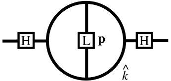
FIG. 5.: A two-loop diagram used to exemplify the decoupling of the replicas using the Schwinger representation.

Let us begin with a concrete example. In the thermodynamic limit, the diagram depicted in Fig. 5 contributes to $A_{n}$ a term proportional to

$$g^{4}\int d^{(n+1)d}{k}\,\,d^{d}{p}\,\,G_{0}({\hat{k}})^{2}\,G_{0}({\bf p})^{2}\,G_{0}({\hat{k}}+{\bf p})^{2}$$ (19)

$$\qquad=g^{4}\int d^{d}{k^{0}}\,\,d^{d}{p}\,\,\int_{\sigma_{1}\sigma_{2}\sigma_{3}}\!\!\!\!\!\!\!\!\!\sigma_{1}\sigma_{2}\sigma_{3}\,{\rm e}^{-(\sigma_{1}+\sigma_{2}+\sigma_{3})r_{0}}{\rm e}^{-(\sigma_{1}+\sigma_{3}){\bf k}^{0}\cdot{\bf k}^{0}}\,{\rm e}^{-(\sigma_{2}+\sigma_{3}){\bf p}\cdot{\bf p}}\,{\rm e}^{-2\sigma_{3}{\bf k}^{0}\cdot{\bf p}}\,\prod_{\alpha=1}^{n}\int d^{d}{k^{\alpha}}\,{\rm e}^{-(\sigma_{1}+\sigma_{3}){\bf k}^{\alpha}\cdot{\bf k}^{\alpha}}$$ (20)

$$\qquad=g^{4}\int d^{d}{k^{0}}\,\,d^{d}{p}\,\,\int_{\sigma_{1}\sigma_{2}\sigma_{3}}\!\!\!\!\!\!\!\!\!\sigma_{1}\sigma_{2}\sigma_{3}\,{\rm e}^{-(\sigma_{1}+\sigma_{2}+\sigma_{3})r_{0}}{\rm e}^{-(\sigma_{1}+\sigma_{3}){\bf k}^{0}\cdot{\bf k}^{0}}\,{\rm e}^{-(\sigma_{2}+\sigma_{3}){\bf p}\cdot{\bf p}}\,{\rm e}^{-2\sigma_{3}{\bf k}^{0}\cdot{\bf p}}\,\left(\int d^{d}{k}\,{\rm e}^{-(\sigma_{1}+\sigma_{3}){\bf k}\cdot{\bf k}}\right)^{n}$$ (21)

$$\qquad\buildrel n\to 0\over{\longrightarrow}g^{4}\int d^{d}{k}\,d^{d}{p}\,\int_{\sigma_{1}\sigma_{2}\sigma_{3}}\!\!\!\!\!\!\!\!\!\sigma_{1}\sigma_{2}\sigma_{3}\,{\rm e}^{-(\sigma_{1}+\sigma_{2}+\sigma_{3})r_{0}}{\rm e}^{-(\sigma_{1}+\sigma_{3}){\bf k}\cdot{\bf k}}\,{\rm e}^{-(\sigma_{2}+\sigma_{3}){\bf p}\cdot{\bf p}}\,{\rm e}^{-2\sigma_{3}{\bf k}\cdot{\bf p}}$$ (22)

$$\qquad=g^{4}\int d^{d}{k}\,\,d^{d}{p}\,\,G_{0}({\bf k})^{2}\,G_{0}({\bf p})^{2}\,G_{0}({\bf k}+{\bf p})^{2}.$$ (23)

This limiting value is precisely that occurring for the corresponding diagram in the HRW field theory for the PT.

The tactic that we have just employed, viz., the use of the Schwinger representation to decouple the replicas from one another, provides easy and explicit access to the replica limit and, hence, to the precise correspondence with the HRW prescription. It can straightforwardly be invoked not only for all diagrams that contribute to the coefficients $A_{n}$ and (by the same procedure) $C_{n}$, but also for the coefficient $B_{n}$.

When considering diagrams contributing to $A_{n}$ and $C_{n}$, we saw that what survived were terms in which all internal LRS wave vectors flowed in a common (but otherwise arbitrary) replica. Now, as we consider $B_{n}$, there is a slight complication arising from the presence of an external wave vector, which spoils the full ${\cal P}_{n+1}$ permutation symmetry. However, this external wave vector has been chosen to lie in replica zero and, as we have shown above, the only surviving contribution is the one in which all internal LRS wave vectors also flow in replica zero. Then, via the Schwinger representation of the propagators, and via factorization on the replica indices, we see that the Feynman integral, in the replica limit, is identical to that in the HRW approach. Hence, the VT presents not only the the same coefficients $A_{0}$ and $C_{0}$ of the two- and three-point vertex functions as does the HRW representation, but also the same coefficient $B_{0}$.

IV Concluding remarks

Let us summarize what is presented in this Paper. We have addressed the vulcanization transition via a minimal field-theoretic model. This model is built from an order parameter whose argument is the $(n+1)$-fold replication of ordinary $d$-dimensional space. [The structure of this theory should be contrasted with that of more familiar replica field theories, in which it is the (internal) components of the field that are replicated rather than the (external) argument]  We have considered appropriate long-wave-length aspects of the two- and three-point vertex functions for this model, to all orders in perturbation theory in the cubic nonlinearity. Via a detailed analysis of the diagrammatic expansion for these quantities, we have found that, in the replica limit, these vulcanization-theory vertex functions precisely coincide with the corresponding vertex functions of a certain field-theoretic representation (due to Houghton, Reeve and Wallace) of the percolation transition. Hence, percolation theory correctly captures the critical phenomenology the liquid and critical states of vulcanized matter.

REFERENCES

- [1] H. E. Castillo, P. M. Goldbart and A. Zippelius, Europhys. Lett. 28, 519 (1994).
- [2] W. Peng, H. E. Castillo, P. M. Goldbart and A. Zippelius Phys. Rev. B 57, 839 (1998).
- [3] H. E. Castillo and P. M. Goldbart, Phys. Rev. E 58, R24 (1998); ibid., E 62, 8159 (2000).
- [4] H. E. Castillo, P. M. Goldbart and A. Zippelius, Phys. Rev. B 60, 14702 (1999).
- [5] P. M. Goldbart, H. E. Castillo and A. Zippelius, Adv. Phys. 45, 393 (1996).
- [6] P. M. Goldbart, J. Phys. Cond. Matt. 12, 6585 (2000).
- [7] W. Peng and P. M. Goldbart, Phys. Rev. E 61, 3339 (2000).
- [8] See, e.g., D. Stauffer and A. Aharony, Introduction to Percolation Theory, Second Edition (Taylor and Francis, Philadelphia, 1991)
- [9] See, e.g., P. J. Flory, Principles of Polymer Chemistry (Cornell University Press, 1953); D. Stauffer, J. Chem. Soc. Faraday Trans. II 72, 1354 (1976); P.-G. de Gennes, Scaling Concepts in Polymer Physics (Cornell University Press, Ithaca, 1979).
- [10] See also T. C. Lubensky and J. Isaacson, Phys. Rev. Lett. 41, 829 (1978); ibid. 42, 410 (1979) (E); Phys. Rev. A 20, 2130 (1979); J. Physique 42, 175 (1981); and D. Stauffer, A. Coniglio, and M. Adam, Adv. in Polym. Sci. 44, 103 (1982).
- [11] A brief account of this work was reported in W. Peng, P. M. Goldbart and A. J. McKane, Bull. Am. Phys. Soc. 46, 1101 (2001).
- [12] A. Houghton, J. S. Reeve and D. J. Wallace, Phys. Rev. B 17, 2956 (1978).
- [13] See Sec. VI of Ref. [7] and Ref. [6] for further remarks on this issue. We thank H. E. Castillo for discussions on this subject.
- [14] H.-K. Janssen and O. Stenull, cond-mat/0103583.
- [15] S. J. Barsky and M. Plischke, Phys. Rev. E 53, 871 (1996); S. J. Barsky, Ph.D. Thesis, Simon Fraser University, Canada (unpublished, 1996); S. J. Barsky and M. Plischke (unpublished, 1997).
- [16] See, e.g., Ref. [5].
- [17] R. T. Deam and S. F. Edwards, Phil. Trans. R. Soc. 280A, 317 (1976).
- [18] The precise correspondence is determined by comparing Eq. (1) of the present Paper with Eq. (5.6) of Ref. [7].
- [19] Strictly speaking, as the wave vector in question is required to be in the HRS, it can not be exactly . Instead, one should conceive of the value at as being the limiting value as via a path in the HRS.
- [20] By this we mean , where is an arbitrary permutation of the replicas.
- [21] See, e.g., M. Le Bellac, Quantum and Statistical Field Theory (Oxford University Press, 1991), Sec. 5.5.3.