Software Corrections of Vocal Disorders

Abstract

We discuss how vocal disorders can be post-corrected via a simple nonlinear noise reduction scheme. This work is motivated by the need of a better understanding of voice dysfunctions. This would entail a twofold advantage for affected patients: Physicians can perform better surgical interventions and on the other hand researchers can try to build up devices that can help to improve voice quality, i.e. in a phone conversation, avoiding any surgigal treatment. As a first step, a proper signal classification is performed, through the idea of geometric signal separation in a feature space. Then through the analysis of the different regions populated by the samples coming from healthy people and from patients affected by T1A glottis cancer, one is able to understand which kind of interventions are necessary in order to correct the illness, i.e. to move the corresponding feature vector from the sick region to the healthy one. We discuss such a filter and show its performance.

Keywords: Vocal Disorders, Embedding Theory, Recurrence Plot, Nonlinear Noise Reduction, Feature Space

PACS: 07.05.Kf, 05.40.Ca, 87.19.Xx, 05.45.Tp

Phase Space Reconstruction

The first simple difference between dysphonic and healthy voices is shown in Fig.1, where the time evolution of the amplitude of a microphone-registered sound is represented. The upper panel could be interpreted as a highly noisy time series, but careful investigations reveal that this is not the case: Applying a simple low-pass filter would only introduce a distortion bigger than the original noise level. Some of the noise-like structures belong to the time series and one has to be able to correctly identify what is worth keeping and what has to be eliminated during the correction procedure.

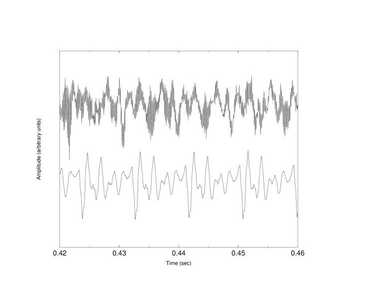
Figure 1: Typical shapes of the investigated time series. Upper panel: Dysphonic voice. Lower panel: Healthy sample.

From a theoretical point of view, this paper relies on the theory of dynamical systems and deterministic chaos; the former implies that the time evolution is defined in some phase space, the latter offers a striking explanation for irregular behaviour and anomalies in systems which do not seem to be inherently stochastic. Even very simple chaotic dynamical systems can exhibit strongly irregular time evolution without random inputs.

Consider for a moment a purely deterministic system. Once its present state is fixed, the states at all future times are determined as well. Thus it will be important to establish a vector space, the so-called phase space, for the system such that specifying a point in this space specifies the state of the system, and vice versa. This implies that we can study the dynamics of the system by studying the dynamics of the corresponding phase space points.

Unfortunately what we observe in an experiment is not a phase space object but a time series, most likely only a scalar sequence of measurements. We therefore have to convert the observations into state vectors: This is the problem of phase space reconstruction which is technically solved by the method of delays or related constructions takens ; sauer ; kantz1 . Most commonly, the time series is a sequence of scalar measurements of some quantity which depends on the current state of the system, considered at multiples of a fixed sampling time:

$$s_{n}=s({\bf x}(n\Delta t))+\eta_{n},$$ (1)

namely we look at the system through some measurement function $s()$ and make observations only up to some random fluctuations $\eta_{n}$, the measurement noise. A delay reonstruction in $m$ dimensions is then formed by the vectors $\beta_{n}$, given as

$$\beta_{n}=(s_{n-(m-1)\nu},s_{n-(m-2)\nu},...,s_{n-\nu},s_{n}).$$ (2)

The time difference in number of samples $\nu$ or in time units $\nu\Delta t$ between adjacent components of the delay vectors is referred to as the lag or delay time.

A number of embedding theorems are concerned with the question under which circumstances and to what extent the geometrical object formed by the vectors $\beta_{n}$ is equivalent to the original trajectory ${\bf x}_{n}$. Here equivalent means that they can be mapped onto each other by a uniquely invertible smooth map and, under quite general circumstances the attractor formed by $\beta_{n}$ is equivalent to the attractor in the unknown space in which the original system is living if the dimension $m$ of the delay coordinate space is sufficiently large.

Recurrence plots of the voice

Human voices form an aperiodic and highly nonstationary signal. A sentence can be decomposed in subunits, called phonemes, which can be considered as different types of dynamics. Careful investigation of time and length scales shows that the sound wave characterizing a single phoneme (duration between 50 and 200 ms) has a characteristic profile (pitch) of about 5-15 ms. A kind of phase angle on this highly nontrivial oscillation will then identify the instantaneous amplitude. Thus a delay reconstruction should allow us to identify the actual phoneme and the phase inside it.

Figure 2: Section of a recurrence plot of the time series in the lower panel of Fig.1. A recurrence plot is constructed on the basis of mutual distances between points belonging to the same trajectory. Every dot in $(i,j)$ implies that $|\beta_{i}-\beta_{j}|<\epsilon$. There are almost no dots for $|i-j|>2000$, reflecting the lack of interphoneme similarities (for this particular choice of $\epsilon$). The occurrence of lines mirrors the deterministic character of the system: It is therefore possible to distinguish between different dynamical regimes, namely to introduce pseudostates in the system.

Looking at the Eq.2 one realizes that at least two parameters are involved in the delay reconstruction from a scalar time series, namely $m$ and $\nu$. Some recipes for an optimal tuning of them are available at the moment, but an adequate theory is still missing; in any case, a good tool is represented by the recurrence plot (see recurrenceplot ; recurrenceplot2 ). This method was used for the first time to study recurrencies and nonstationary behaviour occurring in dynamical systems. It allows to identify system properties that cannot be observed using other linear and nonlinear approaches and it is especially useful for analysis of nonstationary systems with high dimensional and/or noisy dynamics.

Recurrence plots are constructed on the basis of mutual distances between point belonging to the same trajectory. In the plane of indices $i$ and $j$ a dot is printed whenever the delay vectors $\beta_{i}$ and $\beta_{j}$ fulfill the relation $|\beta_{i}-\beta_{j}|<\epsilon$. So a recurrence plot depends also on the parameter $\epsilon$. The Fig.2 proves that our delay vectors really represent meaningful states, where the line structure shows the approximate periodicity inside the phonemes and the number of intraphoneme neighbours.

The distance between two consecutive lines indicates the duration of the basic structure (pitch) inside a phoneme. We can see from Fig.2 that this involves approximately 200 points. Considering that the sentence has been sampled at a 22,05 kHz rate, this implies a profile of about 9 ms. In order to correctly identify such a structure, in the delay reconstruction of Eq.2, the product $\nu m$ (the so-called time window) has to be bigger than 200. A more detailed insight into the role of this two parameters is given in Ref. dimitris .

Nonlinear noise reduction

Noise reduction means that one tries to decompose a time series into two components, one containing the signal, the other random fluctuations. Implicitly we always assume that the data represents an additive superposition of two different components which have to be distinguishable through some objective criterion.

The classical statistical tool for obtaining this distinction is the power spectrum. Random noise has a flat, or at least a broad, spectrum, whereas periodic or quasi-periodic signals have sharp spectral lines. After both components have been identified in the spectrum, a Wiener filter can be used to separate the time series accordingly. This approach fails for our purposes here because the undesirable part of the signal is not what is usually considered to be noise. It is very strongly correlated to the clean part of the signal, indeed it is part of the signal. Even if parts of the spectrum can be clearly associated with the signal, a separation into signal and noise fails for most parts of the frequency domain.

The filter we use has been proposed in lms and arises from the chaotic deterministic systems field, where the determinism yields a criterion to distinguish the signal and the noise (which is supposed not to be deterministic). Let the time evolution of the signal be deterministic with an unknown map $f$. All that we have knowledge of are noisy measurements of this signal:

$$s_{n}=x_{n}+\eta_{n},\hskip 28.45274ptx_{n}=f(x_{n-m},...,x_{n-1}).$$ (3)

Here $s_{n}$ is the scalar time series we can measure, $x_{n}$ the clean signal and $\eta_{n}$ the superimposed noise. In order to obtain an estimate $\hat{x}_{n_{0}-m/2}$ for the value of $x_{n_{0}-m/2}$ we form delay vectors

$${\bf s}_{n}=(s_{n-m+1},...,s_{n})$$ (4)

and determine those which are close to ${\bf s}_{n_{0}}$. The average value of $s_{n-m/2}$ is then used as a cleaned value $\hat{x}_{n_{0}-m/2}$:

$$\hat{x}_{n_{0}-m/2}=\frac{1}{|U_{\epsilon}({\bf s}_{n_{0}})|}\sum_{{\bf s}_{n}\in U_{\epsilon}({\bf s}_{n_{0}})}s_{n-m/2}.$$ (5)

Here $|U_{\epsilon}({\bf s}_{n_{0}})|$ denotes the number of elements of the neighbourhood $U_{\epsilon}({\bf s}_{n_{0}})$ of radius $\epsilon$ around the point ${\bf s}_{n_{0}}$, which is never empty, no matter how small a value of $\epsilon$ we choose: It always contains at least ${\bf s}_{n_{0}}$. This is good to know since we have to make some choice of $\epsilon$ when we use this algorithm. It is guaranteed that if we choose $\epsilon$ too small the worst thing that can happen is that the only neighbour found is ${\bf s}_{n_{0}}$ itself. This, however, yields the estimate $\hat{x}_{n_{0}-m/2}=s_{n_{0}-m/2}$ which just means that no correction is made at all.

To get an impression of how the local projective noise reduction scheme works, assume that one has to eliminate noise from music stored on an old-fashioned long playing record, induced by scratches on the black disc. The task becomes almost trivial if one can make use of several samples of this LP. When playing them synchronously, the signal part of the different tracks id identical, whereas the noise part is independent: As a consequence of that, already a simple averaging would enhance the sound quality. In deterministic chaotic signals, this redundancy is stored in the past: Similar initial conditions will behave in a similar way, at least for short periods. In human voice signals there is no need to suppose a chaotic behavior, since every phoneme is made up of pitches in an almost periodic fashion. This means that every logical unit provides all the redundancy required for its filtering.

How can we make sure that all we do is to reduce noise without distorting the signal? In Fig.1 two typical time series, one related to a healthy voice, the other to a sick one, are compared. In the lower panel we can see the recurrence of structures of length approximately 9 ms inside a phoneme, in total agreement with the recurrence plot analysis. The person who has spoken this sentence is absolutely healthy and the corresponding signal looks very clean. The same repetition is not that clear in the upper panel, where a patient affected by a T1A glottis cancer was asked to say the same group of words in the same environmental conditions, namely in a professional quiet room. The signal looks very noisy, but listening to it one perceives only the sick voice and no indication of noise, at least of what one usually means saying noise.

Spectral analyses show the same result: The vocal disorder reveals itself as a noisy signal, but the nature of this noise is not the conventional one. It is not addivite and it is correlated with the other sub-part of the sentence one would like to isolate. In herzel2 ; ishizaka ; manfredi ; reuter ; pinto ; kumar it is shown how some of the complexities observed in disordered voices are not caused by random external input to the vocal apparatus, but by the intrinsic nonlinear dynamics of vocal fold movement. Normal phonation corresponds to an essentially synchronized motion of all vibratory modes. A change of parameters such as muscle tension or localised vocal fold lesions may lead to a desynchronization of certain modes resulting in the appearance of these new features that look like noise.

The distinction of the signal in a deterministic part and in a stochastic component is then not possible. Nevertheless one would still like to extract the main structure from the signal, suppressing the noise-like features. For this purpose the previously described filter is worth applying to correct the disorders: If we choose suitably the involved parameters we are able to identify the structures inside a phoneme and to perform an average of them via Eq.5. Every point belonging to a structure is replaced by a local average of similar points coming from different structures (this is done searching for neighbours in the embedding space). The resulting signal does not show just an exact repetition of these parts because the averaging procedure acts only locally and the points involved in the computation varies from structure to structure. Also in a normal signal, in fact, the repetitions are not perfect.

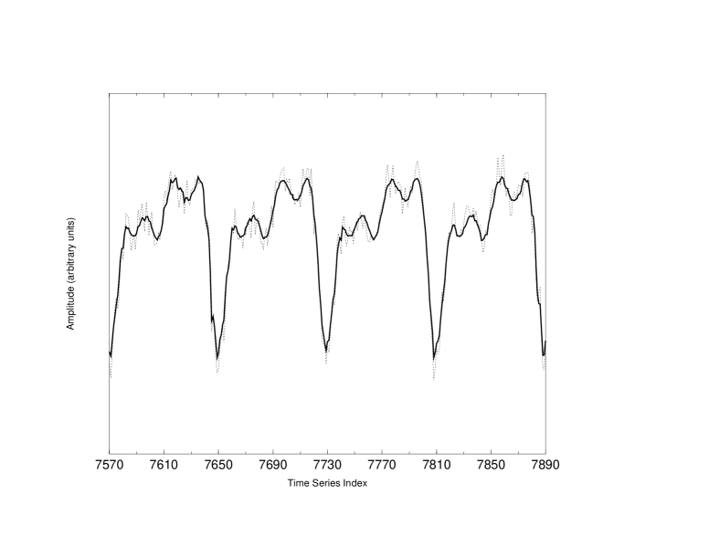
Figure 3: Corrections performed by the nonlinear noise reduction to a dysphonic voice. Dotted line: Original voice. Solid line: Corrected voice.

One has then to be careful when choosing the $\epsilon$: A too big value would result in a drastic averaging and the resulting signal would sound too artificial. On the other hand a small value of $\epsilon$ is not able to perform any correction. In Fig.3 we show what happens when using the filter with a good set of parameters: The main shape of the sub-structures is preserved, but the noise-like features are attenuated. The meaning of good here is the following: The recurrence plot of Fig. 2 shows that the system generating the time series we are analyzing really possesses dynamical regimes. Since we want to be able to distinguish between different states, the vectors $\beta_{n}$ of the delay reconstruction has to comprise all the points belonging to a pitch. So the product $\nu m$ of the lag and the embedding dimension has to be approximately 200 in the example depicted on Fig. 2. A choice of a big $m$ results on big computational efforts; on the other hand a big $\nu$ produces worse results. We refer again to Ref. dimitris for more details. The parameter $\epsilon$ is used for the neighbourood relations between vectors in the embedding space. We draw a point in $(i,j)$ on the recurrence plot if $|\beta_{i}-\beta_{j}|<\epsilon$. The value of $\epsilon$ has to be bigger than the noise level. A good way to tune it is through the recurrence plot: Whit a small $\epsilon$ we get almost no recurrences, a very big $\epsilon$ is such that the relation $|\beta_{i}-\beta_{j}|<\epsilon$ is fulfilled from almost all the vector pairs. The optimal value of $\epsilon$ is mirrored on a recurrence plot where the lines are as long as possible, as thin as possible and all the recurrences belong to lines.

If we tune the parameters according to this recipe, the filtered signal sounds more normal than the original, even if some characteristic aspect of the voice has been lost. In the horizontal axis of Fig.3 we report the index of the time series in order to show the number of points involved in the filtering procedure. Every structure lasts 80 points; in a space of such a dimensionality, the vector having these elements as components is represented as a single point. The four structures of Fig.3 are neighbours because the involved sequences of points are approximately the same. As shown in dimitris , it is not necessary to consider such a big space, but one can skip some intermediate point, taking care to cover the full structure in any case.

Results

We are dealing with three categories of subjects: (i) patients affected by T1A glottis cancer, a tumour confined to the glottis region with mobility of the vocal cords (ii) healthy patients and (iii) patients under medical treatment, operated via endoscopic laser or traditional lancet technique. The sentence spoken by all of them is the italian word aiuole (flower-beds), since it contains a lot of vowels: Patients suffering from dysphonia need a great effort in saying this word.

To classify the sentences we make use of the feature space introduced in fspace , whose components are special quantities extracted from the time series: Spectral factor, pseudo-entropy, pseudo-correlation dimension, first zero-crossing of the autocorrelation function, first Lyapunov exponent, prediction error, jitter, shimmer, peaks in the phoneme transition, residual noise. It is not necessary here to go into details, one has just to know that this space represents the proper object where a good classification of vocal pathologies is feasible.

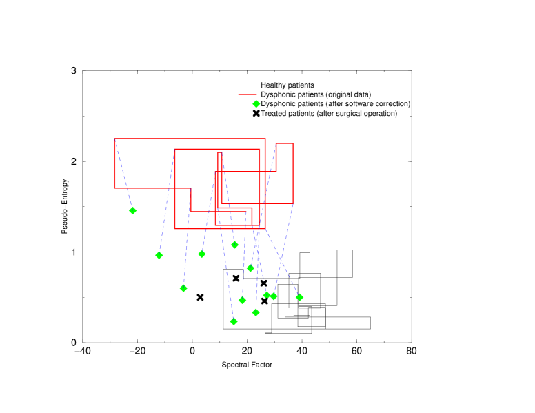
Figure 4: Two-dimensional projection of the feature space. Healthy patients are characterized by a pseudo-entropy close to 0.5 and a spectral factor whitin the range [10,60]. Sick patients populate a region of the feature space where the pseudo-entropy has a value close to 2 and the spectral factor ranges between -30 and 30. A bold cross refers to a patient after a surgical operation. The effect of this treatment is a drastic decrease of the pseudo-entropy and a moderate increase in the value of the spectral factor. Dotted lines link the points before the filtering to the same samples after the proposed software corrections. The algorithm produces similar effects of a surgical treatment.

In Fig.4 we see a projection of the feature space onto the spectral factor and the pseudo-entropy dimensions; we can see how healthy and sick patients populate different regions and which are the results of the medical treatments performed on four patients (indicated by a bold cross). Unfortunately we don’t have samples from the same treated people before the surgical operation, so that it is not possible to link the four cases directly to the pre-operatory phase. The dotted lines link the points before the filtering to the points after the attenuation of the noise-like features. We can force the algorithm to perform a stronger filtering of the dysphonic time series (as explained in the Appendix, this is possible increasing the number of iteration of the correction routine), but one has always to be careful: In order to get a better value of some components of the feature space, one has to come to a compromise with some other quantities and the best answer comes, as usual in these cases, from a direct listening of the time series (after the convertion in a .wav format).

The results shown in Fig.4 have been obtained with the following set of parameters: $m=30$, $\nu=4$ and $\epsilon=0.3\sigma$, with $\sigma$ being the variance of the original data. Dysphonic patients, in the (spectral factor, pseudo-entropy) plane, are spread around the average point (5,1.8); the centre of mass of the healthy cluster is (35,0.5). The surgical treatment produces an average correction located in (20,0.6). Our software moves the centre of mass of sick patients to (15,0.7). In getting these results the value of $m$ and $\nu$ is not so crucial, provided that $m\nu>l_{p}$, being $l_{p}$ the extension of a pitch. The program is more sensitive to the choice of $\epsilon$, in the following way: The length of the dotted line of Fig.4 is somehow proportional to the value of $\epsilon$. Unfortunately the angle is not constant: This means that up to a certain value of $\epsilon$ all the corrections act along the same direction, beyond that threshold they start to deteriorate the voice. In the extreme case of $\epsilon$ as big as the full embedding space, the averaging procedure performed by Eq. 5 would destroy almost completely the signal (producing a pseudo-entropy and a spectral factor close to zero).

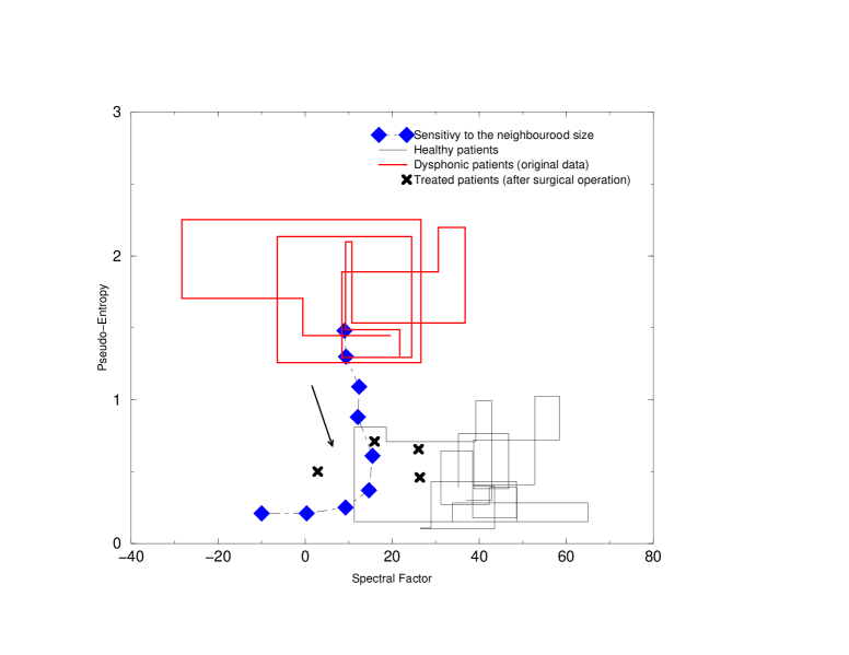
Figure 5: Two-dimensional projection of the feature space. Healthy patients are characterized by a pseudo-entropy close to 0.5 and a spectral factor whitin the range [10,60]. Sick patients populate a region of the feature space where the pseudo-entropy has a value close to 2 and the spectral factor ranges between -30 and 30. The path followed by the bold diamands is the effect of corrections with increasing $\epsilon$ ($\epsilon$ increases along the direction indicated by the arrow). $\epsilon=0$ coincides with the original sample, since no neighbour can be identified and therefore no correction is performed. The last three points are the result of a filtering with a too big neighbourood size. Only for two values of $\epsilon$ the corrected time series lies in the healthy region.

The sensitivity of the program to the choice of $\epsilon$ is illustrated in Fig. 5. There we have filtered one sample with 8 different values of the neighbourood size. The original position is the one with the biggest value of the pseudo-entropy. $\epsilon$ is increasing along the direction indicated by the arrow and only for two values of it the corrected point lies in the healthy region. For the last three corrections the neighbourood size was absolutely too big. The other samples behave in a qualitatively similar way.

Conclusions

To summarize, we have proposed a procedure to correct numerically some kind of vocal disorders. The main ingredients are the theory of dynamical systems, the delay reconstruction from a scalar measurement, the method of recurrence plot and a nonlinear noise reduction scheme. We also make use of a feature space in order to visualize the results of the filtering procedure. A detailed description of how the idea has been implemented is also provided in Appendix. We have discussed the meaning, implications, methodology and mathematical background of the most relevant parameters and the sensitivity of the program to their choice. The software corrections perform an improvement on the voice quality that is comparable to what a surgical operation is able to do. This suggests the idea of implementing the procedure in a physical device able to help people correcting their voice, without having to undergo a medical treatment.

Appendix: Implementation outline

We present here the sketch of the subroutine filter written in a pseudo-C code. We skip all the details related to the syntax of the programming language for a better readability.

void show_options(char *progname)
{
  fprintf(stderr,"\t-m embedding dimension [Default: 5]\n");
  fprintf(stderr,"\t-T max distance in time [Default: no limit]\n");
  fprintf(stderr,"\t-d delay [Default: 1]\n");
  fprintf(stderr,"\t-r minimal neighbourhood size \n\t\t"
Ψ  "[Default: (interval of data)/1000]\n");
  fprintf(stderr,"\t-R maximal neighborhoodsize[Default: not set]\n");
  fprintf(stderr,"\t-i # of iterations [Default: 1]\n");
}

The input of the program has to be a scalar time series corresponding to the amplitude of the voice signal. Every conventional ASCII file is accepted with the data in one column. The parameter $m$ is the embedding dimension (typical values in the range $[20,40]$), $T$ is the portion of the time series where to look for neighbours: Since every pitch gets neighbours only within the same phoneme, the typical value of $T$ is 2000 (with a sampling rate of 22,05 kHz, 2000 points are almost 100 ms, approximately the length of a phoneme). The parameter $d$ is the time delay, usually in the range $[3,10]$ such that the product $md$ is as big as the length of a pitch. The size of the neighbourood $\epsilon$ is specified through $r$ and $R$, its minimal and maximal value respectively: $r$ should equal the noise level and $R$ is usually $1.5r$. With the parameter $i$, number of iterations, one can set the strength of the filtering. Tipically we use $i=1$.

unsigned long lfind_neighbors(long act,double eps)
{
  k=(int)((searchdim-1)*delay);
  k1=(int)((searchdim/2)*delay);
  i=(int)(series[act-k]/eps)&ib;
  j=(int)(series[act-k1]/eps)&ib;
  n=(int)(series[act]/eps)&ib;

  for (i1=i-1;i1<=i+1;i1++) {
    i2=i1&ib;
    for (j1=j-1;j1<=j+1;j1++) {
      j2=j1&ib;
      for (n1=n-1;n1<=n+1;n1++) {
Ψelement=box[i2][j2][n1&ib];
Ψwhile (element != -1) {
Ψ  if (labs(act-element) < maxdist) {
Ψ    dx=0.0;
Ψ    for (k=0;k<searchdim;k++) {
Ψ      k1= k*(int)delay;
Ψ      dx += fabs(series[act-k1]-series[element-k1]);
Ψ    }
Ψ    if (dx/(double)searchdim <= eps) {
Ψ      dist[nf]=dx;
Ψ      flist[nf++]=element;
Ψ    }
Ψ  }
Ψ  element=list[element];
Ψ}
      }
    }
  }
  return nf;
}

Two points in the embedding space are considered neighbours if (labs(act-element) $<$ maxdist). For every point we build here a list containing all its neighbours. We do it firstly in a two dimensional space to speed up the process. If two points are neighbours in a five dimensional space, this relation holds also in two dimension. Of course the opposite is not true.

void correct(unsigned long n)
{
  epsinv=1./eps;
  for (i=0;i<dim*delay;i++)
    hcor[i]=0.0;

  i=(int)(series[n-(dim-1)*delay]*epsinv)&ibox;
  j=(int)(series[n]*epsinv)&ibox;

  for (i1=i-1;i1<=i+1;i1++) {
    i2=i1&ibox;
    for (j1=j-1;j1<=j+1;j1++) {
      element=box[i2][j1&ibox];
      while (element != -1) {
Ψif (labs(n-element) < maxdist) {
Ψ  for (k=0;k<dim;k++) {
Ψ    k1=k*delay;
Ψ    dx=fabs(series[n-k1]-series[element-k1]);
Ψ    if (dx > eps)
Ψ      break;
Ψ  }
Ψ  if (k == dim) {
Ψ    flist[nfound++]=element;
Ψ    for (k=0;k<dim*delay;k++)
Ψ      hcor[k] += series[element-k];
Ψ  }
Ψ}
Ψelement=list[element];
      }
    }
  }
  for (k=0;k<dim*delay;k++) {
    corr[n-k] += (hcor[k]=series[n-k]-hcor[k]/nfound);
    nf[n-k]++;
  }
  for (i=0;i<nfound;i++) {
    j=flist[i];
    for (k=0;k<dim*delay;k++) {
      trend[j-k] += hcor[k];
      tcount[j-k]++;
    }
  }
}

The second to last for iteration performs exactly what indicated in Eq.5. The variable nfound is $|U_{\epsilon}({\bf s}_{n_{0}})|$.

int main(int argc,char **argv)
{
  series=(double*)get_series(infile,&length,exclude,column,1);

  rescale_data(series,length,&d_min,&d_max);

  resize_eps=0;
  for (iter=1;iter<=iterations;iter++) {
    epsilon=mineps;
    all_done=0;
    epscount=1;
    allfound=0;
    fprintf(stderr,"Starting iteration %d\n",iter);
    while(!all_done) {
      put_in_box(epsilon);
      all_done=1;
      for (n=(searchdim)*delay-1;n<length;n++)
Ψif (!ok[n]) {
Ψ  nfound=lfind_neighbors(n,epsilon);
Ψ  if (nfound >= minn) {
Ψ    correct(n);
Ψ    ok[n]=epscount;
Ψ    if (epscount == 1)
Ψ      resize_eps=1;
Ψ    allfound++;
Ψ  }
Ψ  else
Ψ    all_done=0;
Ψ}
      fprintf(stderr,"Corrected %ld points with epsilon= %e\n",allfound,
Ψ      epsilon*d_max);
      epsilon *= epsfac;
      epscount++;
      if (epsilon > maxeps)
Ψbreak;
    }

    sprintf(ofname,"%s.%d",outfile,iter);
    file=fopen(ofname,"w");
    fprintf(stderr,"Opened %s for writing\n\n",ofname);
    for (i=0;i<length;i++) {
      fprintf(file,"%e\n",series[i]*d_max+d_min);
      if (stdo && (iter == iterations))
Ψfprintf(stdout,"%e\n",series[i]*d_max+d_min);
    }
    fclose(file);
  }
  return 0;
}

The flow is the following: Get the time series, rescale it to a proper interval, apply the filter (call to the function correct) a iter number of times, print the corrected time series to a new data file.

References

- (1) F. Takens. Detecting strange attractors in turbulence. Lecture Notes in Mathematics, Vol. 898, Springer, New York (1981).
- (2) T. Sauer, J. Yorke and M. Casdagli. Embedology. J. Stat. Phys. 65 579 (1991).
- (3) H. Kantz and T. Schreiber. Nonlinear time series analysis. Cambridge University Press, Cambridge (UK), (1997).
- (4) J.P. Eckmann, S. Oliffson Kamphorst and D. Ruelle. Recurrence plot. Europhys. Lett. 4, 973 (1987).
- (5) M. Casdagli. Recurrence plot revisited. Physica D 108, 206 (1997).
- (6) D. Kugiumtzis. State space reconstruction parameters in the analysis of chaotic time series - the role of the time window length. Physica D 95, 13 (1995).
- (7) R. Hegger, H. Kantz and L. Matassini. Denoising Human Speech Signals using Chaoslike Features. Phys. Rev. Lett. 84, 3197 (2000).
- (8) H. Herzel, D. Berry, I.R. Titze and M. Saleh. Analysis of Vocal Disorders with Methods from Nonlinear Dynamics. Journal of Speech and Hearing Research 37, 1008-1019 (1994).
- (9) K. Ishizaka and J.L. Flanagan. Synthesis of voiced sounds from a two-mass model of the vocal cords. Bell. Syst. Tech. J. 51, 1233-1268 (1972).
- (10) C. Manfredi, P. Bruscaglioni, M. D’Aniello, L. Pierazzi and A. Ismaelli. Pitch and noise estimation in hoarse voices. Proc. Int. Workshop on Models and Analysis of Vocal Emissions for Biomedical Applications, Firenze, 42-47 (1999).
- (11) R. Reuter, H. Herzel and R. Orglmeister. Simulations of Vocal Fold Vibrations with an Analog Circuit. Int. J. Bifurcation and Chaos 9, 1075-1088 (1999).
- (12) N.B. Pinto and I.R. Titze. Unification of perturbation measures in speech signals. Journal of the Acoustical Society of America 87, 1278-1289 (1990).
- (13) A. Kumar and S.K. Mullick. Nonlinear dynamical analysis of speech. J. Acoust. Soc. Am. 100, 615-629 (1996).
- (14) L. Matassini, C. Manfredi, R. Hegger and H. Kantz. Analysis of Vocal Disorders in a Feature Space. Medical Engineering and Physics 22, 413-418 (2000).